Reconstructing ultrafast energy-time entangled two-photon pulses
Jean-Philippe W. MacLean, Sacha Schwarz, Kevin J. Resch

TL;DR
This paper introduces a novel method to reconstruct the joint spectral amplitude of ultrafast energy-time entangled photon pairs using a modified Gerchberg-Saxton algorithm, enabling better measurement and control of quantum optical fields.
Contribution
It presents a new technique for reconstructing ultrafast entangled photon pulses from joint measurements, tailored for weak quantum fields unlike classical laser pulses.
Findings
Successful reconstruction of two-photon energy-time entangled states
Enhanced measurement capabilities for ultrafast quantum optical fields
Potential applications in quantum information processing
Abstract
The generation of ultrafast laser pulses and the reconstruction of their electric fields is essential for many applications in modern optics. Quantum optical fields can also be generated on ultrafast time scales, however, the tools and methods available for strong laser pulses are not appropriate for measuring the properties of weak, possibly entangled pulses. Here, we demonstrate a method to reconstruct the joint-spectral amplitude of a two-photon energy-time entangled state from joint measurements of the frequencies and arrival times of the photons, and the correlations between them. Our reconstruction method is based on a modified Gerchberg-Saxton algorithm. Such techniques are essential to measure and control the shape of ultrafast entangled photon pulses.
Click any figure to enlarge with its caption.
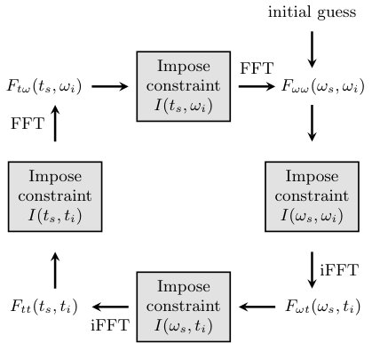 Figure 1
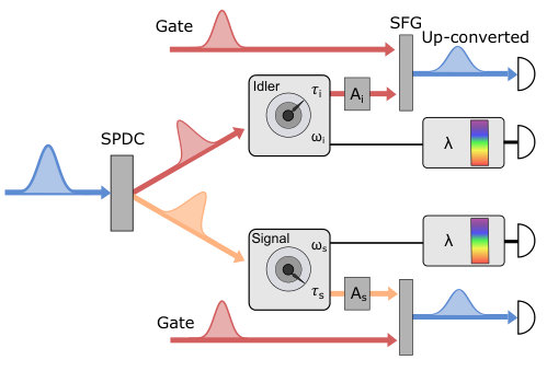 Figure 2
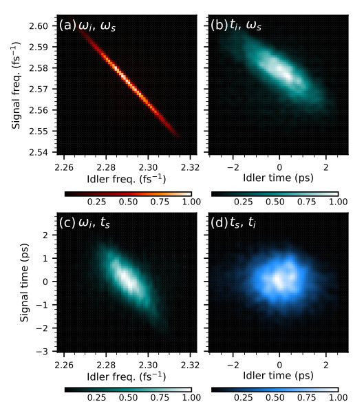 Figure 3
 Figure 4
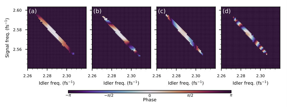 Figure 5
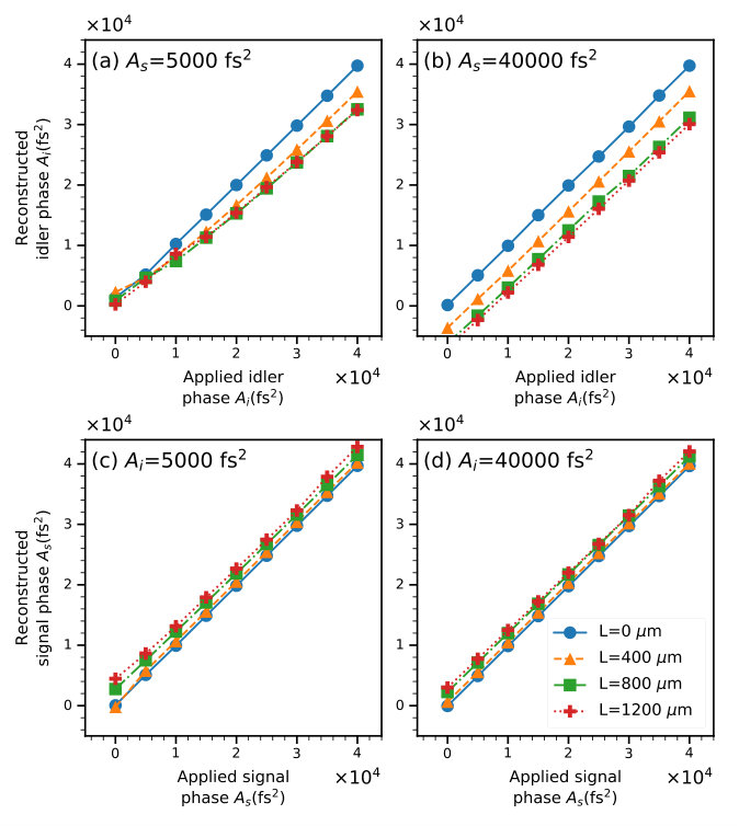 Figure 6
Peer Reviews
No public reviews on file for this paper yet. If you reviewed it on a platform where reviews are public (OpenReview, ICLR, NeurIPS, ICML), you can paste yours below so the community can read it here.
Videos
No videos yet. Explain this paper in a talk, walkthrough, or lecture? Add one.
Reconstructing ultrafast energy-time entangled two-photon pulses
Jean-Philippe W. MacLean
Institute for Quantum Computing, University of Waterloo, Waterloo, Ontario, Canada, N2L 3G1
Department of Physics & Astronomy, University of Waterloo, Waterloo, Ontario, Canada, N2L 3G1
Sacha Schwarz
Institute for Quantum Computing, University of Waterloo, Waterloo, Ontario, Canada, N2L 3G1
Department of Physics & Astronomy, University of Waterloo, Waterloo, Ontario, Canada, N2L 3G1
Kevin J. Resch
Institute for Quantum Computing, University of Waterloo, Waterloo, Ontario, Canada, N2L 3G1
Department of Physics & Astronomy, University of Waterloo, Waterloo, Ontario, Canada, N2L 3G1
Abstract
The generation of ultrafast laser pulses and the reconstruction of their electric fields is essential for many applications in modern optics. Quantum optical fields can also be generated on ultrafast time scales, however, the tools and methods available for strong laser pulses are not appropriate for measuring the properties of weak, possibly entangled pulses. Here, we demonstrate a method to reconstruct the joint-spectral amplitude of a two-photon energy-time entangled state from joint measurements of the frequencies and arrival times of the photons, and the correlations between them. Our reconstruction method is based on a modified Gerchberg-Saxton algorithm. Such techniques are essential to measure and control the shape of ultrafast entangled photon pulses.
I Introduction
The generation, control, and measurement of high-dimensional entangled quantum states of light are important for optical computing and communication Lanyon et al. (2009); Kues et al. (2017); Cai et al. (2017); Sparrow et al. (2018). One form of this entanglement, in the energy-time degree of freedom, can exhibit strong correlations in frequency and time van Loock and Furusawa (2003); Shalm et al. (2013), nonlocal interference phenomena Franson (1989); Kwiat et al. (1993), and dispersion cancellation Franson (1992); Wasak et al. (2010), with applications in high-capacity quantum key distribution Nunn et al. (2013); Zhong et al. (2015), enhanced spectroscopy Raymer et al. (2013), sensing Zhang et al. (2015), and two-photon absorption Dayan et al. (2004). The generation and control of energy-time entanglement has been realized in both bulk crystals and waveguide structures Kang et al. (2014); Donohue et al. (2016, 2018); Arzani et al. (2018); Ansari et al. (2018a), however, it remains an important challenge to reconstruct the quantum state of the photons produced. The performance of any quantum optical technology using time and frequency depends on being able to both shape and completely characterize such photonic states.
In ultrafast optics and laser physics, the ability to measure the amplitude and phase of laser pulses on ultrafast timescales is essential for nonlinear optics and spectroscopy. In this context, the problem of electric field reconstruction has been extensively studied Walmsley and Dorrer (2009). Optical pulses can be produced on time scales much shorter than any photodetector response time Keller (2003), and consequently, the only thing fast enough to measure an ultrafast laser pulse is another ultrafast pulse. Techniques such as FROG Kane and Trebino (1993) and SPIDER Iaconis and Walmsley (1998) make use of nonlinear optical processes to measure and reconstruct ultrafast pulses. However, adapting them to quantum states of light is challenging due to the low power levels of single photons. In addition, the algorithms developed for laser pulses do not account for the possibility that photons can be entangled. New innovations are therefore needed to reconstruct the joint state of entangled ultrafast photon pulses.
Approaches for characterizing the optical modes of photons have been explored using homodyne measurements Lvovsky and Raymer (2009); Lvovsky et al. (2001); Aichele et al. (2002); Polycarpou et al. (2012); Morin et al. (2013); Qin et al. (2015), two-photon interference effects Chen et al. (2015); Tischler et al. (2015); Tiedau et al. (2018), and two-photon absorption in semiconductors Boitier et al. (2011). The increased interest in time-frequency modes has also led to nonlinear ultrafast approaches for characterization Ansari et al. (2017, 2018b); Davis et al. (2018a, b). To measure both the frequency and time intensity correlations of energy-time entangled states, optical methods based on optical gating and frequency resolved measurements have recently been developed. These have been used to observe nonlocal dispersion cancellation MacLean et al. (2018a) and two-photon quantum interferometry MacLean et al. (2018b) on time scales inaccessible to standard photodetectors. For complete characterization, however, the joint spectral phase is also required. This additional phase information is important to understand the nature of the entanglement and to control and optimize the performance of quantum information protocols using heralded and multi-photon states Zielnicki et al. (2018).
Recovering the phase of a field from intensity measurements in Fourier-related domains is known as a phase-retrieval problem. In 1972, Gerchberg and Saxton provided a practical solution to this problem. They introduced an iterative algorithm, referred to as the Gerchberg-Saxton algorithm (GS), to extract the complete wavefunction of an electron beam, including its phase, from intensity recordings in the image and diffraction planes Gerchberg and Saxton (1972). Their algorithm can be applied to problems involving electromagnetic waves Fienup (2013); Shechtman et al. (2015) including optical wavelengths Peri (1987).
In this paper, we implement a technique to recover the phase of ultrafast energy-time entangled two-photon pulses produced via spontaneous parametric downconversion (SPDC) and which is based on intensity measurements of the frequency and the arrival time of the photons. Inspired by the conventional phase retrieval problem, we develop an algorithm based on a method of alternate projections Gerchberg and Saxton (1972); Fienup (1978, 1982) that iterates between the frequency and time domains imposing the measured intensity constraints at each iteration. Measurements in frequency are performed with single-photon spectrometers and measurements in time are implemented via optical gating with an ultrafast optical laser pulse.
II Theory
A pure energy-time two photon state produced via SPDC can be modelled as Shalm et al. (2013); Donohue et al. (2016),
[TABLE]
corresponding to a superposition of frequency modes for the signal and the idler weighted by the joint spectral amplitude (JSA) function . The joint spectral amplitude,
[TABLE]
describes the amplitude, , and phase, , of the state. For downconversion, it is related to the pump properties and the phase matching conditions of the nonlinear material Mosley et al. (2008). In this form, the joint-spectral intensity characterizes the frequency correlations, whereas the joint temporal amplitude (JTA),
[TABLE]
which is related to the JSA by the Fourier transform, and the corresponding joint temporal intensity (JTI), , characterize the temporal correlations. Energy-time entanglement is then witnessed when the time-bandwidth product is found to be less than one, , where represents the standard deviation in the joint spectral and joint temporal intensity Mancini et al. (2002); Cho et al. (2014); MacLean et al. (2018a).
One is typically interested in determining the complex-valued functions or , but only has access to their intensities, or . The GS algorithm was originally designed to recover the phase from two similar intensity measurements. However, phase retrieval algorithms of this form have a well-known ambiguity. If the intensity distribution in the Fourier plane is centro-symmetric, then the complex conjugate of any given solution in the object plane is also a solution Guizar-Sicairos and Fienup (2012). For the energy-time degree of freedom, this implies a time-reversal ambiguity, i.e., it is not possible to distinguish between positive and negative dispersion from the intensity correlations in frequency and time, and , alone. In the present work, we measure properties of entangled photons and can naturally include other time-frequency correlations,
[TABLE]
which can distinguish between these two cases and break the time-reversal ambiguity.
III Phase retrieval algorithm
The phase retrieval algorithm is shown in Fig. 1. The algorithm is seeded with an initial guess of the state, , involving a random phase. In the first iteration, we project the state onto the constraint set that satisfies the measured intensities in frequency. This is achieved by replacing the spectral amplitudes with the measured spectral amplitudes but keeping the phase,
[TABLE]
We then apply the Fast Fourier Transform algorithm (FFT) to obtain an estimate of and again replace the amplitudes with the measured amplitudes . This is repeated two more times, as in Fig. 1, completing one iteration of the algorithm. At each iteration, we evaluate the FROG-trace error Trebino (2012) between the measured and the reconstructed joint spectral intensities, which corresponds to the average percentage error in each point . An important feature of these types of algorithms is that the measured error will always decrease or remain constant at each iteration, and will not diverge Gerchberg and Saxton (1972); Saxton (2013).
IV Experiment
The setup is schematically depicted in Fig. 2 and described in detail in Refs. MacLean et al. (2018a, b). Ti:sapphire laser pulses [80 MHz, 775 nm, 3.8 W average power, 0.130 ps (s.d.) pulse width], are frequency doubled in 2 mm of -bismuth borate (BiBO). After spectral filtering with a 0.2 nm FHWM bandpass filter, the second harmonic pumps a 5 mm BiBO crystal for type-I SPDC generating energy-time entangled photons at 823 nm and 732 nm. These are coupled in single-mode fibres allowing for direct, spectrally resolved, or temporally resolved measurements. Spectral measurement are performed via monochromators with a resolution of 0.1 nm. Temporal measurements are implemented via optical gating, i.e., via noncollinear sum-frequency generation (SFG) with femtosecond laser pulses in 1 mm of bismuth borate (BiBO) crystal. The electric field of the gate pulse is characterized using an SHG-FROG measurement, and we find an intensity pulse width of 130 fs (s.d.). Since the experimentally measured intensity in frequency (time) is convolution of the joint spectral (temporal) intensity and the filter function of the monochromater (temporal gate), the measured data must first be deconvolved before it can be used in the phase-retrieval algorithm. Numerical deconvolutions for each intensity measurement are performed using a Wiener filter Press et al. (2007), and the resulting output provides the intensity distributions, , used in the algorithm in Fig. 1. See Appendix A for further details.
The spectral phase on the photons,
[TABLE]
is controlled with a combination of normally dispersive single-mode fibre and adjustable grating compressor for anomalous dispersion MacLean et al. (2018a), where and are the chirp parameters for the signal and idler, respectively. The relative position of the gratings inside the compressor sets the magnitude and sign of the overall dispersion. We calibrate both grating compressors using XFROG (Cross-correlation FROG) spectrogram measurements between the strong gate pulse and a weak laser pulse. The weak laser pulse has the same center wavelength and path through the fibre-compressor system as the photons on each side. The phase at each relative grating separation is reconstructed using the Principal Component Generalized Projection (PCGP) FROG algorithm Kane (1999); Trebino (2012). We find a quadratic phase that depends linearly on the grating separation with slopes of fs2/mm and fs2/mm for the signal and idler, respectively. The difference between the two is attributed to the cubic dependence on wavelength of dispersion in a grating compressor Treacy (1969).
V Phase reconstructions
We compare the phase retrieval algorithm on measured data for two-photon states with different amounts of dispersion. We set the grating compressors on the signal and idler side to study four cases: no additional dispersion, with extra positive dispersion applied to the idler, with extra negative dispersion applied to the signal, and with extra negative dispersion applied on both sides. For the case of a two-photon energy-time entangled state with negative dispersion applied to both photons, an example of the four combinations of time and frequency measurements is shown in Fig. 3. Background subtraction, a Wiener Filter, and low-pass filters are applied in Fig. 3 and prior to the reconstruction Fittinghoff et al. (1995). We observe strong anti-correlations in the joint spectral intensity [Fig. 3(a)], however, the joint temporal intensity [Fig. 3(d)] is uncorrelated due to the presence of dispersion on both photons. The observed shears in both the time-frequency intensity plots [Fig. 3(b-c)] also illustrate the presence of negative dispersion.
We map these intensity constraints onto a 64x64 array and input them into the phase retrieval algorithm, which is run for 1000 iterations, a number found heuristically after which no reduction in the FROG-trace error is observed. The intensity of the reconstructed wavefunction in frequency and time are shown in Fig. 4. The reconstructed intensities are compared to the measured data from Fig. 3(a) and Fig. 3(d). We find a FROG-trace error between the post-processed and reconstructed spectral intensities after 1000 iterations to be for the joint spectral intensity and for the joint temporal intensity.
Note that the marginal bandwidths of the joint spectral intensity in the reconstruction [Fig. 4(a)] are shorter than in the original data [Fig. 3(a)]. Numerical simulations suggest that this arises as a result of the phase-matching bandwidth in the optical gating. The effect of the phase mismatch on the reconstruction of two-photon states with optical gating is modelled in Appendix B.
Fig. 5 shows the reconstructed joint spectral phase for the four different cases. Starting with the case where we attempted to minimize the unbalanced dispersion [Fig. 5(a)], we observe a relatively flat spectral phase. In this configuration, we measure the time-bandwidth product as in Ref. MacLean et al. (2018a) and find , verifying the presence of energy-time entanglement.
For the three cases where dispersion is applied, we fit the reconstructed quadratic spectral phase in Fig. 5(b-d). For each, we unwrap the 2D phase and perform a polynomial fit to the phase distribution. The corresponding uncertainties are obtained from the variance in the fitted spectral phase after performing Monte Carlo simulations assuming Poissonian noise.
When we apply ps2 of dispersion on the signal photon [Fig. 5(b)], we reconstruct a quadratic spectral phase on the signal of ps2, observing a positive quadratic variation in the phase along the signal (y) axis, modulo 2, with little variations along the idler (x) axis. When we apply ps2 of dispersion to the idler photon [Fig. 5(c)], we reconstruct a quadratic phase on the idler of ps2, observing a negative quadratic variation in the spectral phase along the idler (x) axis, with again little variations along the signal (y) axis. When we apply ps2 and ps2 of dispersion to the signal and idler [Fig. 5(d)], we reconstruct a quadratic phase on the signal and idler of ps2 and ps2, respectively. For this case, we observe a negative quadratic variation along the diagonal x-y axis.
When dispersion is applied to only one photon, Fig. 5(b) and Fig. 5(c), the phase obtained using the phase-retrieval algorithm corresponds to the reconstructed phases measured using the XFROG algorithm. In the last case, Fig. 5(d), we find a discrepancy between the two. This, again, is likely due to the effect of the phase mismatch on the temporal measurements and on the subsequent reconstruction of two-photon states, which will be more pronounced for the photons which have much larger bandwidth than for the weak pulse used for the XFROG reconstructions (see Appendix B).
VI Conclusion
We have demonstrated a method to recover ultrafast two-photon energy-time entangled pulses. Our technique is based on a method of alternate projections that iterates between the frequency and time domains imposing the measured intensity constraints at each iteration. The use of nonlinear phenomena, i.e., optical gating, to measure the timing correlations is an artifact of the time scales at play and is not a fundamental requirement. For sufficiently long pulses, there may exist photodetectors that can measure the temporal intensity directly Korzh et al. (2018). For subpicosecond resolution involving optical gating, the effect of phase-matching in the upconversion could be reduced using shorter crystals or angle-dithering O’Shea et al. (2000).
In our simulations, the reconstruction fidelity seems to depend on the amount of entanglement in the initial state, and uncovering the reason for this is the subject of future work. Moreover, extensions of this algorithm to characterize two-photon mixed states may be possible based on techniques used to reconstruct partially coherent light Thibault and Menzel (2013); Bourassin-Bouchet and Couprie (2015), removing assumptions about the purity of the quantum states. Measurement and reconstruction capabilities similar to those available in ultrafast optics will be essential for developing new applications in quantum state engineering and ultrafast shaping of entangled photons, paving the way to characterizing and manipulating high-dimensional quantum states of light.
The authors thank J.M. Donohue and F. Miatto for fruitful discussions. This research was supported in part by the Natural Sciences and Engineering Research Council of Canada (NSERC), Canada Research Chairs, Industry Canada and the Canada Foundation for Innovation (CFI).
Appendix A Phase retrieval algorithm
The algorithm to reconstruct the phase of energy-time entangled states is divided into two main parts: post-processing and phase retrieval. In the first part, post-processing, for each experimentally measured time-frequency correlation plot, the data is interpolated onto a 2D square grid, , of size 64x64, where, here, we use to represent either the measured time or frequency variables. We apply background subtraction using a corner suppression routine Trebino (2012). The numerical deconvolution is performed using a Wiener filter,
[TABLE]
where is the filter function which we obtain by taking the Fourier transform of the instrument response functions. These are approximated as Gaussian functions with the instrument resolutions obtained experimentally for the spectral (0.1 nm) and temporal (0.130 ps) measurements. The parameter takes into account the amount of noise in the system and will typically depend on and . Here, we approximate it as a constant, , which is obtained heuristically for each reconstruction. A low-pass filter is also applied by multiplying the Wiener filter by a top-hat function of radius, in pixels, and setting all the values outside to 0, where is the size of the grid, and . The deconvolved intensities are then obtained with the inverse Fourier transform,
[TABLE]
where is the Fourier Transform of the experimentally measured intensities . The resulting deconvolved intensities are used as the physical constraints in the phase retrieval algorithm.
In the second part, the phase retrieval algorithm is seeded with an initial guess of the state, which can consist of the measured amplitudes with a random phase. Steps (1-8) are used when all four intensity constraints are applied.
Replace the magnitude of with the measured values
[TABLE] 2. 2.
Evaluate the inverse Fourier transform to obtain an estimate of . 3. 3.
Replace the magnitude of with the measured values
[TABLE] 4. 4.
Evaluate the inverse Fourier transform to obtain an estimate of . 5. 5.
Replace the magnitude of with the measured values
[TABLE] 6. 6.
Evaluate the Fourier transform to obtain an estimate of . 7. 7.
Replace the magnitude of with the measured values
[TABLE] 8. 8.
Evaluate the Fourier transform to obtain an estimate of .
The time to run the algorithm depends on the size of the arrays being used and the number of iterations. For the case in Fig. 4, using a 64x64 array, the entire procedure, including loading the data, applying filtering and deconvolution algorithms, and running the phase retrieval algorithm for 1000 iterations takes about s, averaged over 100 runs and using a laptop computer (i7-4650U CPU @2.3GHz with 8 Gb of RAM).
Appendix B Reconstructing two-photon states with optical gating
To test the numerical deconvolution and the phase-reconstruction algorithm described above using realistic temporal measurements, we construct a numerical model of optical gating with thick crystals and consider its effect on the measurement and reconstruction of energy-time entangled two-photon states.
An energy-time entangled two-photon state as in Eq. 1 with a joint-spectral amplitude for the signal and idler frequencies is modelled with a two-dimensional correlated Gaussian function,
[TABLE]
The marginal frequency bandwidths, and , are set to the values measured experimentally. The correlation parameter describes the statistical correlations between the frequency of the signal and idler modes and is related to the purity of the partial trace, . When , the joint-spectral amplitude factorizes and the state is separable, whereas when , the photons are perfectly anticorrelated in frequency. Furthermore, when the marginal bandwidths are equal, , the time-bandwidth product for the Gaussian state in Eq. 14 is . We apply a quadratic phase to the state,
[TABLE]
where and are the chirp parameters on the signal and idler, respectively.
In the SFG process used for optical gating, a photon and a strong gate pulse in the near-infrared (NIR) are up-converted to produce a higher energy photon in the ultraviolet. If the photons are dispersed before the optical gating, high and low frequencies components will arrive at different times in the nonlinear medium. In the presence of phase mismatch, the upconverted frequencies associated to these high and low frequency components can lie outside the phase-matching bandwidth of the crystal, and consequently will be suppressed. As a result, phase mismatch in optical gating changes the measured intensity correlations and therefore changes the deconvolved intensity constraints that are applied in the phase retrieval algorithm.
To account for this effect, we model the optical gating as sum-frequency generation process in the low-efficiency regime between the photons on each side and a gate pulse with centre frequency and a pulse duration of 0.130 ps, leading to upconverted frequencies and on the signal and idler side, respectively. The gate pulse is modeled with a Gaussian temporal profile,
[TABLE]
with marginal bandwidth , and delay . For the purpose of this simulation, we assume the spectral measurements have high resolution such that they can be represented by delta functions,
[TABLE]
and the three intensity measurements involving optical gating are calculated via the following,
[TABLE]
where the gate pulse is the same on both sides but with delays and introduced. The phase matching function is
[TABLE]
where the phase-mismatch,
[TABLE]
is calculated for type-I SFG with different crystal lengths and the experimentally measured wavelengths. The phase-matching bandwidth can be estimated from the range of frequencies contained in . Upconverted frequencies outside this range are suppressed. All integrals are evaluated numerically.
We model all the steps in the phase-retrieval process. We numerically create frequency anti-correlated states using Eq. 14 and Eq. 15, with the same centre wavelength and bandwidth as those measured experimentally, but with different amounts of applied spectral phases, given by the chirp parameters and . We calculate the four joint correlations in frequency and time with Eqs. (17-20) using different lengths of BiBO for optical gating, apply the numerical deconvolution to each intensity measurement as described in Appendix A, and insert these as constraints for the phase retrieval algorithm. After reconstruction, we unwrap the spectral phase of the reconstructed joint spectral amplitude function and fit it to a third-order two-dimensional polynomial.
The reconstructed spectral phases are compared to the applied spectral phases in Fig. 6 for different lengths of BiBO used in optical gating and for different applied spectral phases. In Fig. 6(a) and Fig. 6(b), the signal chirp parameter is kept fixed while the idler chirp parameter is varied, whereas in Fig. 6(c) and Fig. 6(d), the idler chirp parameter is kept fixed while the signal chirp parameter is varied. When the length of the crystal is set to zero ( m), the reconstructed phase corresponds exactly to the applied phase, and the line at m appears at 45 degrees with a slope of one. As the length of the crystal increases, we find that the slope remains fairly constant at 45 degrees, but the offset depends on the configuration. For example, comparing Fig. 6(a) and Fig. 6(b), we find the values of the reconstructed idler chirp parameter depend on whether the signal chirp parameter has a value of fs2 [Fig. 6(a)] or fs2 [Fig. 6(b)]. The difference between the reconstructed and applied phase in Fig. 6 also becomes larger for longer crystals where the phase matching function is more restrictive.
The reference list from the paper itself. Each links out to its DOI / PubMed record.
- 1Lanyon et al. (2009) B. P. Lanyon, M. Barbieri, M. P. Almeida, T. Jennewein, T. C. Ralph, K. J. Resch, G. J. Pryde, J. L. O’Brien, A. Gilchrist, and A. G. White, Nat. Phys. 5 , 134 (2009) . · doi ↗
- 2Kues et al. (2017) M. Kues, C. Reimer, P. Roztocki, L. R. Cortés, S. Sciara, B. Wetzel, Y. Zhang, A. Cino, S. T. Chu, B. E. Little, D. J. Moss, L. Caspani, J. Azaña, and R. Morandotti, Nature 546 , 622 (2017) . · doi ↗
- 3Cai et al. (2017) Y. Cai, J. Roslund, G. Ferrini, F. Arzani, X. Xu, C. Fabre, and N. Treps, Nat. Commun. 8 , 15645 (2017) . · doi ↗
- 4Sparrow et al. (2018) C. Sparrow, E. Martín-López, N. Maraviglia, A. Neville, C. Harrold, J. Carolan, Y. N. Joglekar, T. Hashimoto, N. Matsuda, J. L. O’Brien, D. P. Tew, and A. Laing, Nature 557 , 660 (2018) . · doi ↗
- 5van Loock and Furusawa (2003) P. van Loock and A. Furusawa, Phys. Rev. A 67 , 052315 (2003) . · doi ↗
- 6Shalm et al. (2013) L. K. Shalm, D. R. Hamel, Z. Yan, C. Simon, K. J. Resch, and T. Jennewein, Nat. Phys. 9 , 19 (2013) . · doi ↗
- 7Franson (1989) J. D. Franson, Phys. Rev. Lett. 62 , 2205 (1989) . · doi ↗
- 8Kwiat et al. (1993) P. G. Kwiat, A. M. Steinberg, and R. Y. Chiao, Phys. Rev. A 47 , R 2472 (1993) . · doi ↗