Hamiltonisation, measure preservation and first integrals of the multi-dimensional rubber Routh sphere
Luis C. Garc\'ia-Naranjo

TL;DR
This paper extends the analysis of a rolling sphere problem to multiple dimensions, demonstrating measure preservation, Hamiltonian structure, and conserved quantities using recent geometric methods.
Contribution
It generalizes the multi-dimensional rubber Routh sphere problem and establishes Hamiltonian structure and first integrals using Chaplygin's reducing multiplier method.
Findings
Reduced equations have an invariant measure.
System can be expressed in Hamiltonian form.
Existence of conserved quantities for the system.
Abstract
We consider the multi-dimensional generalisation of the problem of a sphere, with axi-symmetric mass distribution, that rolls without slipping or spinning over a plane. Using recent results from Garc\'ia-Naranjo (arXiv: 1805:06393) and Garc\'ia-Naranjo and Marrero (arXiv: 1812.01422), we show that the reduced equations of motion possess an invariant measure and may be represented in Hamiltonian form by Chaplygin's reducing multiplier method. We also prove a general result on the existence of first integrals for certain Hamiltonisable Chaplygin systems with internal symmetries that is used to determine conserved quantities of the problem.
Click any figure to enlarge with its caption.
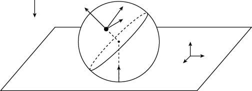 Figure 1
Peer Reviews
No public reviews on file for this paper yet. If you reviewed it on a platform where reviews are public (OpenReview, ICLR, NeurIPS, ICML), you can paste yours below so the community can read it here.
Videos
No videos yet. Explain this paper in a talk, walkthrough, or lecture? Add one.
Hamiltonisation, measure preservation and first integrals of the multi-dimensional rubber Routh sphere111This research was made possible by a Georg Forster Experienced Researcher Fellowship from the
Alexander von Humboldt Foundation that funded a research stay of the author at TU Berlin.
Luis C. García-Naranjo
Abstract
We consider the multi-dimensional generalisation of the problem of a sphere, with axi-symmetric mass distribution, that rolls without slipping or spinning over a plane. Using recent results from García-Naranjo [22] and García-Naranjo and Marrero [23], we show that the reduced equations of motion possess an invariant measure and may be represented in Hamiltonian form by Chaplygin’s reducing multiplier method. We also prove a general result on the existence of first integrals for certain Hamiltonisable Chaplygin systems with internal symmetries that is used to determine conserved quantities of the problem.
Contents
-
2.1 Nonholonomic Chaplygin systems and the gyroscopic tensor
-
2.4 -simple Chaplygin systems, measure preservation and Hamiltonisation
1 Introduction
An important contribution of S. A. Chaplygin to the field of nonholonomic systems was the introduction of the so-called Chaplygin’s reducing multiplier method [10]. It is concerned with a certain class of nonholonomic systems with symmetry, commonly referred to today as nonholonomic Chaplygin systems, whose reduced equations of motion have the form of a classical mechanical system subjected to extra gyroscopic forces. Chaplygin’s method consists of searching for a time reparametrisation hoping that in the new time variable, and after a momentum rescaling, the extra forces vanish and the resulting system is Hamiltonian. If successful, this process is often referred to as Chaplygin Hamiltonisation. It is also common to say that the Chaplygin system at hand, in the original time variable, is conformally Hamiltonian. The subclass of Chaplygin systems allowing a Chaplygin Hamiltonisation is quite remarkable, and substantial effort has been devoted to their study and characterisation (see e.g. [10, 26, 37, 7, 17, 11, 4, 19, 22] and references therein). The purpose of this paper is to provide a new non-trivial example within this category, and to prove a considerably general Noether-type of result for these systems, which links their internal symmetries with first integrals, and which we apply to our example.
-simple Chaplygin systems: Hamiltonisation and first integrals.
Our approach to Chaplygin Hamiltonisation relies on the notion of -simple Chaplygin systems introduced recently in García-Naranjo and Marrero [23]. These systems form an exceptional subclass of nonholonomic Chaplygin systems that always possess an invariant measure and allow a Chaplygin Hamiltonisation.
The definition of -simple Chaplygin systems relies on a certain tensor field of type defined on the shape space222the shape space is the quotient manifold where is the configuration manifold of the system and is the underlying symmetry group of the Chaplygin system. of the system, which measures the interplay between the kinetic energy and the non-integrability of the constraint distribution. This tensor field already appears in the works of Koiller [31] and Cantrijn et al [9], and, following the terminology of [22, 23], will be called the gyroscopic tensor. A Chaplygin system is said to be -simple if there exists a function such that the gyroscopic tensor satisfies333throughout the paper we denote by the action of the vector field on the scalar function .
[TABLE]
for any two vector fields on . The above condition was obtained as the coordinate-free formulation of the recent results on Chaplygin Hamiltonisation given recently by the author [22]. It is shown in [23] that the condition to be -simple is equivalent to the verification of certain sufficient conditions for Chaplygin Hamiltonisation given previously by Stanchenko [37] and Cantrijn et al [9]. The advantage of the formulation in [22] and [23] with respect to these references is that condition (1.1) can be systematically examined in concrete examples.
The statement that a -simple Chaplygin system allows a Chaplygin Hamiltonisation is independent of the number of degrees of freedom of the problem, and may be interpreted as a generalisation of the celebrated Chaplygin’s Reducing Multiplier Theorem [10]
- whose applicability is restricted to systems whose shape space has dimension - see the discussion in [22] and [23].
The criterion of -simplicity has already been used in [22] and [23] to establish the Hamiltonisation of non-trivial examples. Among them is the multi-dimensional Veselova problem whose Hamiltonisation was first proven by Fedorov and Jovanović [17, 18] by a direct application of Chaplygin’s method to the reduced equations of motion. In Section 4 of this paper we prove that the multi-dimensional rubber Routh sphere (introduced below) is also -simple. This allows us to prove that the system allows a Chaplygin Hamiltonisation, and to give a closed formula for its invariant measure, without writing the equations of motion. Our results seem to support the thesis that -simplicity is the relevant mechanism behind the Chaplygin Hamiltonisation of concrete examples.444this statement is meant within the framework of Hamiltonisation of Chaplygin systems. Other examples, like the remarkable Hamiltonisation of the Chaplygin sphere obtained by Borisov and Mamaev [5], involve a further symmetry reduction [7] and other geometric mechanisms come into play to ensure that invariant first integrals descend to the quotient space as Casimir functions [21].
In Section 3 we prove a general result that shows how extra symmetries of -simple Chaplygin systems leads to the existence of conserved quantities (Theorem 3.1). This result is applied to find first integrals of the multi-dimensional rubber Routh sphere in Section 4.3. This contributes to the recent efforts to understand the mechanisms responsible for the existence of first integrals that are linear in velocities in nonholonomic mechanics (see e.g. [25, 12, 13, 2]).
The multi-dimensional rubber Routh sphere
Routh [36] considered the problem of a sphere, whose distribution of mass is axially symmetric, that rolls without slipping on the plane. Later, Borisov and Mamaev [6, 8] considered the problem under an additional rubber555the rubber terminology for constraints that prohibit spinning goes back to Ehlers et al [11] and Koiller and Ehlers [32] and is now quite standard in the field. constraint that forbids spinning. In this paper we consider the multi-dimensional generalisation of this system. Our terminology multi-dimensional rubber Routh sphere is supposed to indicate the presence of a no-spin constraint in the word rubber, and the axi-symmetric assumption on the mass distribution of the sphere with the mention of Routh’s name. A closely related problem is the multi-dimensional rubber Chaplygin sphere considered by Jovanović [28].
The study of multi-dimensional systems in nonholonomic mechanics goes back to Fedorov and Kozlov [16], and has received wide attention as a source of interesting examples for integrability, Hamiltonisation and other types of dynamical features [38, 27, 17, 18, 29, 30, 14, 15, 20]. Our analysis of the multi-dimensional rubber Routh sphere contributes to enlarge this family of examples.
Structure of the paper
In Section 2 we present a quick review of the recent constructions in [22, 23]. This summary includes the definition of the gyroscopic tensor of and its expression in local coordinates. We also recall the notion of -simplicity (described above) and, in Theorem 2.5, we indicate its precise relationship with measure preservation and Hamiltonisation. Section 3 is completely devoted to Theorem 3.1 that relates internal symmetries of -simple Chaplygin systems to first integrals. Section 4 is concerned with the multidimensional rubber Routh sphere. To simplify the reading, we first treat the 3D system in subsection 4.1 and then proceed to the D generalisation in subsection 4.2. The -simplicity of the system is presented in Theorem 4.6 and the consequential measure preservation and Hamiltonisation properties in Corollary 4.8. The results of Section 3 are then applied to determine first integrals of the problem in subsection 4.3. The paper finishes with an Appendix A that contains the proof of a technical lemma needed in the proof of Theorem 4.6.
2 Preliminaries: a review of -simple Chaplygin systems and their measure preservation
and Hamiltonisation properties
In this section we briefly recall the notion of nonholonomic Chaplygin systems and, more specifically, -simple Chaplygin systems introduced in García-Naranjo and Marrero [23], together with their measure preservation and Hamiltonisation properties.
2.1 Nonholonomic Chaplygin systems and the gyroscopic tensor
For our purposes, a ** nonholonomic system** is a triple . Here is an -dimensional smooth manifold modelling the configuration space of the system. is a vector sub-bundle whose fibres define a non-integrable distribution on of constant rank , that models linear nonholonomic constraints as follows: a curve on is said to satisfy the constraints if and only if for all . Finally, is the Lagrangian of the system that is assumed to be of mechanical type, namely
[TABLE]
where the kinetic energy defines a Riemannian metric on , and is the potential energy.
The triple contains all the information for the evolution of the system in accordance with the Lagrange-D’Alembert principle of ideal constraints. The (velocity) phase space of the system is and the dynamics is described by the flow of a uniquely defined vector field . An intrinsic definition of this vector field may be found, for instance, in [33].
Definition 2.1**.**
The nonholonomic system is said to be a Chaplygin system if there exists an ()-dimensional Lie group acting freely and properly on and satisfying the following properties:
- (i)
acts by isometries with respect to the kinetic energy metric , and the potential energy is invariant, 2. (ii)
is invariant in the sense that for all and , 3. (iii)
for all the following direct sum splitting holds
[TABLE]
where denotes the Lie algebra of , and is the tangent space to the orbit through at .
Remark 2.2**.**
Chaplygin systems as defined above are also referred to in the literature as non-abelian Chaplygin systems [31], generalised Chaplgyin systems [9, 17] or the principal kinematic case of a nonholonomic system with symmetries [3].
The smooth -dimensional manifold associated to a Chaplygin system is called the shape space. As a consequence of the first and second conditions in Definition 2.1, the vector field describing the dynamics is equivariant (with respect to the -action on defined by the restriction of the tangent lifted action of to ) and the system admits a -reduction. The reduced dynamics is described by the flow of the reduced vector field on the orbit space . For a Chaplygin system, the reduced phase space is naturally identified with the tangent bundle , or cotangent bundle , using the (reduced) Legendre transform. The reduced equations of motion have the form of a mechanical system on the shape space subject to gyroscopic forces. Geometrically, they may be written in almost symplectic form, i.e. in Hamiltonian-like form, , where is the reduced Hamiltonian (energy), but where the non-degenerate 2-form on fails, in general, to be closed. See section 2.3 below or references [11, 17, 24, 23] for more details.
We now recall the definition of the gyroscopic tensor from García-Naranjo and Marrero [23]. To do this, we first note that the kinetic energy metric defines the orthogonal decomposition . We shall denote by
[TABLE]
the bundle projection associated to such decomposition. Next we note that, as was first pointed out by Koiller [31], the second and third conditions in Definition 2.1 imply that the fibres of are the horizontal spaces of a principal connection on the principal bundle . As is well known, corresponding to such principal connection, there is a well defined horizontal lift that associates to any vector field an equivariant vector field taking values on , and that is -related to . We are now ready to present:
Definition 2.3**.**
The gyroscopic tensor is the skew-symmetric tensor field on determined by assigning to the vector fields , the vector field , given by
[TABLE]
for , and where is any point such that , and where denotes the Jacobi-Lie bracket of vector fields.
That is a well-defined tensor field on is shown in [23, Proposition 3.4]. It is also shown in this reference that the gyroscopic tensor coincides with other tensor fields that had been considered before by Koiller [31] and Cantrijn et al [9].
2.2 Local expressions for the gyroscopic tensor
Let be local coordinates on the shape space . Then we may write
[TABLE]
for certain -dependent coefficients , which, in view of the skew-symmetry of , are skew-symmetric with respect to the lower indices, i.e. . Following the terminology introduced in García-Naranjo [22], we refer to as the gyroscopic coefficients.
Fix . The gyroscopic coefficients , , may be computed in practice by solving the following linear system of equations:
[TABLE]
where we recall that is the kinetic energy metric on , and we have denoted
[TABLE]
Note that the matrix is invertible by linear independence of . That (2.2) holds is a direct consequence of the definition (2.1) of the gyroscopic tensor since .
2.3 The reduced equations of motion
We now present the reduced equations of motion of a Chaplygin system. Our exposition mainly follows García-Naranjo [22].
The distribution interpreted as a principal connection on the principal bundle , induces a Riemannian metric on that will be denoted by . For it is defined by
[TABLE]
and is locally given by with defined by (2.3). Similarly, the invariance of the potential energy induces a reduced potential such that . Therefore, there is a well defined reduced Lagrangian , of mechanical type, defined by
[TABLE]
Locally we have . As was announced above, the reduced equations of motion take the form of a mechanical system on which is subject to gyroscopic forces. These may be written in terms of the gyroscopic coefficients as (see e.g. [22]):
[TABLE]
Now use the standard Legendre transformation:
[TABLE]
and define the reduced Hamiltonian
[TABLE]
where are the entries of the inverse matrix of . It is a standard exercise to show that Eqs. (2.6) are equivalent to the following first order system on :
[TABLE]
Eqs. (2.9) give the local expression of the reduced vector field on . As mentioned above, this vector field satisfies where the almost-symplectic 2-form
[TABLE]
We refer the reader to [23] for an intrinsic construction of using the gyroscopic tensor. A different, yet equivalent, approach to the construction of is taken in [11].
2.4 -simple Chaplygin systems, measure preservation and Hamiltonisation
In this subsection we recall the recent results on Chaplygin Hamiltonisation from García-Naranjo [22] and García-Naranjo and Marrero [23]666As shown in [23], these results are equivalent to certain sufficient conditions for Hamiltonisation given first by Stanchenko [37] and Cantrijn et al. [9].. We begin with the following:
Definition 2.4** ([23]).**
A non-holonomic Chaplygin system is said to be -simple if there exists a function such that the gyroscopic tensor satisfies
[TABLE]
for all .
The class of -simple Chaplygin systems is quite special. As it turns out, their reduced equations on always possess an invariant measure and allow a Hamiltonisation by Chaplygin’s reducing multiplier method. More precisely:
Theorem 2.5** ([23]).**
- (i)
The reduced equations of motion (2.9) of a -simple Chaplygin system possess the invariant measure , where is the Liouville measure on and . 2. (ii)
The reduced equations of motion (2.9) of a -simple Chaplygin system become Hamiltonian after the time reparametrisation .
The implication of item (i) of the theorem is clear. If the Chaplygin system under consideration is -simple, then Eqs. (2.9) preserve the volume form on whose local expression is
[TABLE]
One interpretation of item (ii)
- followed in [23] - is that -simplicity implies that the 2-form is conformally symplectic with conformal factor . In other words, the 2-form is closed and hence symplectic. Hence, the rescaled vector field satisfies and is therefore Hamiltonian (with respect to the symplectic structure ).
Another, equivalent, interpretation of item (ii) of Theorem 2.5 - followed in [22] - is obtained by defining the momentum rescaling:
[TABLE]
and writing the reduced Hamiltonian in the new variables
[TABLE]
Item (ii) of Theorem 2.5 states that, for a -simple Chaplygin system, Eqs. (2.9) are written in the variables in conformally Hamiltonian form
[TABLE]
The conformal factor may be absorbed in the time reparametrisation leading to the Hamiltonian system:
[TABLE]
3 Noether’s Theorem for -simple Chaplygin systems
We now show how additional - sometimes called internal - symmetries of -simple Chaplygin systems lead to first integrals. This is a consequence of the conformally Hamiltonian structure of their reduced equations. As we show below, the conserved quantities are simply a rescaling by the conformal factor of the standard momentum map for Hamiltonian systems.
We begin by recalling some standard notation. Suppose that the Lie group , with Lie algebra , acts on . For we denote by the infinitesimal generator of . Namely, is the vector field on defined by
[TABLE]
Theorem 3.1**.**
Consider a -simple Chaplygin system and suppose that the Lie group acts on the shape space and leaves invariant.
- (i)
If the reduced Lagrangian defined by (2.5) is invariant under the tangent lifted action of to , then the rescaled tangent bundle momentum map
[TABLE]
is constant along the flow of the reduced equations (2.6). 2. (ii)
If the reduced Hamiltonian defined by (2.8) is invariant under the cotangent lifted action of to , then the rescaled cotangent bundle momentum map
[TABLE]
where denotes the duality pairing between and , is constant along the flow of the reduced equations (2.9). 3. (iii)
Items (i) and (ii) are equivalent via the Legendre transformation (2.7).
Proof.
Let and suppose that in local coordinates . The rescaled tangent bundle momentum map is locally given by:
[TABLE]
which, in view of the Legendre transformation (2.7), coincides with
[TABLE]
which is the local expression for the rescaled cotangent bundle momentum map. So the definitions of in items (ii) and (iii) are indeed matched by the Legendre transformation. The equivalence between the invariance assumptions on and - with respect to the appropriate lifted action of - is quite standard (see e.g. [34]). We complete the proof by showing that, under the cotangent lift invariance assumption on , given by (3.2) is indeed a first integral of Eqs. (2.9). We begin by using the assumption of -simplicity to rewrite Eqs. (2.9) as
[TABLE]
Indeed, a calculation based on the chain rule shows that the above system is equivalent to Eqs. (2.11). Therefore, using the above equations, we compute
[TABLE]
On the other hand, the -invariance of implies
[TABLE]
Moreover, recall (see e.g. [34]) that the cotangent lift of is the vector field on expressed in bundle coordinates as . Therefore, the assumption that is invariant under the cotangent lift of to implies
[TABLE]
Substitution of (3.4) and (3.5) into (3.3) proves the result.
∎
4 The rubber Routh sphere
Routh considered the motion of a sphere, whose distribution of mass is axially symmetric, that rolls without slipping on the plane. Here we enforce an additional rubber constraint that forbids spinning and consider the multi-dimensional generalisation of the system. The 3D version of the problem was already considered by Borisov and coauthors in the works [6, 8] which treat more general problems of 3D bodies that roll without slipping or spinning over a surface.
4.1 The 3D case
Consider a sphere that rolls without slipping or spinning on the plane. The orientation of the sphere is determined by an orthogonal matrix that relates a body fixed frame to an inertial or space frame . We assume that space frame is chosen in such a way that the plane where the rolling takes place is spanned by and , and will denote the space coordinates of the geometric centre by , where the constant is the sphere’s radius. The position and orientation of the sphere is hence completely determined by the pair so the configuration space of the system is . To simplify the exposition, we will denote an element as a pair with . This amounts to the identification of with the embedded submanifold of defined by the holonomic constraint .
Denote by the angular velocity vector of the sphere written in the space frame, and by the same vector written in the body frame. As is well known, these vectors correspond to the right and left trivialisations of the tangent velocity vector as follows
[TABLE]
where , the space of skew-symmetric real matrices, is the Lie algebra of .
The no-slip rolling constraint is written as
[TABLE]
where , denotes the vector product in and denotes the so-called Poisson vector that gives body coordinates of the vector that is normal to the plane where the rolling takes place. The sphere is also subject to the no-spin or rubber constraint
[TABLE]
where denotes the scalar euclidean product in . The first two components of Eq. (4.2) together with Eq. (4.3) define 3 independent nonholonomic constraints that determine a rank 2 distribution on .
Inspired by Routh [36], we assume that the mass distribution of the sphere is axially symmetric. The body frame is chosen with origin at the centre of mass and with aligned with the axis of symmetry. This choice of body frame implies that the inertia tensor of the body is represented by a matrix of the form , with principal moments of inertia . We denote by the distance between and the geometric centre and assume that the coordinates of in the body frame are , see Figure 4.1. The space coordinates of are hence given by the vector . Considering that , where is the Euclidean norm in , the Lagrangian of the system , given by the kinetic minus the potential energy, may be written as
[TABLE]
where is the mass of the sphere, is the gravitational constant, and denotes the third component of , i.e. .
In Eq. (4.4), and in what follows, we write a generic element of as the quadruple , which is possible by the identification of with via the left trivialisation, and the embedding , , induced from the holonomic constraint .
The evolution of the system is clearly independent of horizontal translations and rotations of the space frame about . This corresponds to a symmetry action of the euclidean group on the configuration space as we now show. We represent the group as the Lie subgroup of consisting of matrices of the form
[TABLE]
with . The action of given above on an element is
[TABLE]
This action restricts to since it preserves the holonomic constraint .
Proposition 4.1**.**
The problem of the rubber Routh sphere that rolls without slipping or spinning on the plane is a Chaplgyin system with acting on via Eq. (4.5).
Remark 4.2**.**
Proposition 4.1 is valid even if the sphere fails to be axially symmetric. In fact, it continues to hold for the problem of an arbitrary rubber smooth convex body that rolls without slipping or spinning on the plane.
Proof.
The tangent lifted action is
[TABLE]
Moreover, given that , it follows that the Poisson vector is invariant. Using this, and the above expression for the tangent lift, it is immediate to see that both the rolling (4.2) and rubber (4.3) constraints are invariant. Similarly, one checks that the kinetic and potential energies of the Lagrangian (4.4) are invariant so the conditions (i) and (ii) in Definition 2.1 hold. In order to check that condition (iii) in Definition 2.1 also holds, note that the Lie algebra in our representation is spanned by the matrices
[TABLE]
The infinitesimal generators of and are vector fields on that correspond to pure translations along the and axis respectively, which violate the rolling constraint (4.2). On the other hand, the infinitesimal generator of is a vector field on having constant , which violates the rubber constraint (4.2). Hence, the group orbit is transversal to the constraint distribution and, by a dimension count, the condition (iii) in Definition 2.1 is also verified. ∎
The shape space is diffeomorphic to the two dimensional sphere and the orbit projection is
[TABLE]
where we recall that is the Poisson vector. Note that we realise
[TABLE]
It follows from our discussion in section 2 that the reduced equations of motion are defined on the cotangent bundle .
Theorem 4.3**.**
The problem of the rubber Routh sphere that rolls without slipping or spinning on the plane is -simple with given by
[TABLE]
It follows from item (i) in Theorem 2.5, that the reduced equations on possess the invariant measure:
[TABLE]
where is the Liouville volume form on . Additionally, item (ii) in Theorem 2.5 implies that the reduced system on is conformally Hamiltonian with time reparametrisation:
[TABLE]
Remark 4.4**.**
The invariant measure for the problem was first given by Borisov and Mamaev in [6] (see also [8]). The Hamiltonisation of the system may be deduced as a consequence of the celebrated Chaplygin’s Reducing Multiplier Theorem [10] since the shape space has dimension 2. For the multi-dimensional version of the problem considered below, these properties can no longer be deduced from known results and we will rely on Theorem 2.5.
We do not present a proof of Theorem 4.3 since it is a particular instance of Theorem 4.6 below.
4.2 The D case
We consider a multi-dimensional generalisation of the problem considered in the previous section. Namely, an -dimensional rigid body of spherical shape, with axially symmetric distribution of mass, that rolls without slipping or spinning on a horizontal (with respect to gravity) hyperplane on .
The orientation of the sphere is determined by a rotation matrix that specifies the attitude of the sphere by relating a body fixed frame and a space frame . In analogy with the 3D case, we assume that the rolling takes place on the hyperplane spanned by and that the geometric centre of the sphere has space coordinates , where the constant is the sphere’s radius. We will also assume, as in the 3D case, that the body frame has its origin at the centre of mass and is aligned with the symmetry axis of the sphere. The orientation of is such that the body coordinates of are . The configuration space of the problem is . In analogy to the 3D case, we will work with the embedding of in defined by the holonomic constraint .
As is well known, for the angular velocity can no longer be represented as a vector, but rather as an element in the Lie algebra of . We denote by the representation of the angular velocity in the space frame and by its representation in the body frame. These are related to the right and left trivialisation of the tangent vector by
[TABLE]
and satisfy , where is the adjoint operator.
The constraint of rolling without slipping is that the contact point of the sphere with the hyperplane has zero velocity at every time, and is expressed as the following natural generalisation of (4.2):
[TABLE]
where , and the Poisson vector is now given by . On the other hand, the generalisation of the no-spin rubber constraint (4.3) is that the space representation of the angular velocity satisfies
[TABLE]
In other words, has the form
[TABLE]
where above denotes the zero matrix. The constraints (4.9) were considered by Jovanović [28] in the treatment of the multi-dimensional rubber Chaplygin sphere. They generalise the 3D rubber constraint (4.3) in the following sense: rotations of the sphere that occur on 2-dimensional planes that do not contain the normal vector to the hyperplane where the rolling takes place are forbidden.
Our next step is to give a multi-dimensional generalisation of the Lagrangian (4.4). For this matter we recall that for an -dimensional rigid body the inertia tensor of the body is an operator
[TABLE]
where is the so-called mass tensor of the body, which is a symmetric and positive definite matrix (see e.g. [35]). Our assumption that the mass distribution is axially symmetric, and that the axis of the body frame is aligned with the symmetry axis, imply that, with respect to our choice of body frame, the mass tensor has the form
[TABLE]
Similar to our treatment of the 3D case, we shall represent elements of as quadruples with and . This is done by identifying via the left trivialisation, and by embedding putting and The Lagrangian of the multi-dimensional system is
[TABLE]
where is the euclidean norm in , and is the Killing metric in :
[TABLE]
In (4.12) we continue to denote by the distance of the centre of mass to the geometric centre .
In analogy to the 3D case, there is a symmetry action of the group which we represent as the Lie subgroup of consisting of matrices of the form
[TABLE]
with . The action of given above on an element looks identical to Eq. (4.5), namely
[TABLE]
As in the 3D case, the action restricts to since the holonomic constraint is invariant. In analogy with Proposition 4.1 we have:
Proposition 4.5**.**
The -dimensional generalisation of the problem of the rubber Routh sphere that rolls without slipping or spinning on a hyperplane is a Chaplgyin system with acting on via Eq. (4.13).
The proof is analogous to that of Proposition 4.1 and we omit the details. Also, in analogy with Remark 4.2, we mention that the conclusion of Proposition 4.5 is independent of our symmetry assumptions on the mass distribution of the sphere and also applies to general rubber multi-dimensional convex rigid bodies that roll without slipping or spinning on a horizontal hyperplane in .
The shape space of the system is diffeomorphic to the dimensional sphere , and the orbit projection (4.6), valid in 3D, generalises automatically to
[TABLE]
where we recall that in the the Poisson vector , and we realise by its embedding in :
[TABLE]
As a consequence of our discussion in section 2, the -reduced equations of motion live on the cotangent bundle . We now state our main result which, in view of Theorem 2.5, implies that the multi-dimensional rubber Routh sphere has an invariant measure and allows a Hamiltonisation.
Theorem 4.6**.**
The -dimensional rubber Routh sphere that rolls without slipping or spinning on a horizontal hyperplane is -simple with given by
[TABLE]
Remark 4.7**.**
The conclusion of the above theorem is consistent with Theorem 4.3 by noting that, in the 3D case, the principal moments of inertia are related to the entries of the mass tensor by the relations and .
As a direct consequence of Theorem 2.5 and Theorem 4.6 we obtain:
Corollary 4.8**.**
The -reduced equations on of the -dimensional rubber Routh sphere that rolls without slipping or spinning on a horizontal hyperplane possess the invariant measure:
[TABLE]
where is the Liouville volume form on . Moreover, such reduced system is conformally Hamiltonian with time reparametrisation:
[TABLE]
Proof.
The conclusion about the invariant measure follows from Eq. (4.15) and item (i) of Theorem 2.5 (putting ). The conformally Hamiltonian structure of the equations of motion follows from item (ii) of Theorem 2.5. ∎
The rest of the paper is devoted to prove Theorem 4.6 via a coordinate calculation. The strategy is to follow the steps outlined in section 2.2 to compute the gyroscopic coefficients . We will work with the local coordinates777throughout this section, and in contrast with our notation in section 2, we use sub-indices instead of super-indices on the coordinates on . valid on the northern , or southern , hemispheres of by the relations:
[TABLE]
Associated to the embedding of in , there is an embedding of in given by
[TABLE]
where is the Euclidean scalar product in . Under the above identification, and regardless of the hemisphere under consideration, the coordinate vector fields are given in terms of the canonical vectors , by
[TABLE]
For the rest of the section, given , we identify
[TABLE]
using the left trivialisation of and the usual identification . Therefore, a vector field on is represented as an assignment that to a pair with , associates a pair that satisfies . We will also find it useful to denote
[TABLE]
In accordance with the notation of section 2.2 we denote by the horizontal lift of the coordinate vector field . Namely,
[TABLE]
The following proposition gives an explicit expression for .
Proposition 4.9**.**
Let and , (i.e. ). The horizontal lift
[TABLE]
Proof.
The rubber constraints (4.9) imply for a vector that may be assumed to be perpendicular to . Hence,
[TABLE]
where is perpendicular to . On the other hand, differentiating gives . Whence, and we conclude that
[TABLE]
The rolling constraint (4.8) then implies
[TABLE]
Therefore, we get the following expression for the horizontal lift
[TABLE]
The result then follows by using (4.17). ∎
The following lemma gives expressions, that involve the horizontal lifts and the kinetic energy metric , that will be used below to compute the gyroscopic coefficients . Its proof is postponed to Appendix A.
Lemma 4.10**.**
For we have
[TABLE]
and
[TABLE]
where is the Kronecker delta.
We are now ready to prove the following lemma that gives explicit expressions for the gyroscopic coefficients in our coordinates.
Lemma 4.11**.**
For we have
[TABLE]
Proof.
Using
[TABLE]
it follows, in view of (4.21) and (4.22), that as given by (4.23) satisfy
[TABLE]
In other words, the expressions (4.23) for are the unique solution to the system (2.2) that determines the gyroscopic coefficients. ∎
We are now ready to present:
Proof of Theorem 4.6.
Lemma 4.11 implies
[TABLE]
Considering that , we have for , and hence, from the expression (4.15) for we compute
[TABLE]
Therefore, Eq. (4.24) may be rewritten as
[TABLE]
The above expression, together with the tensorial properties of , shows that the -simplicity condition (2.10) holds on the open dense subset of where . By continuity, it holds on all of . ∎
Remark 4.12**.**
We note that the notion of -simplicity, and hence also our conclusions about measure preservation and Hamiltonisation, only depends on the kinetic energy and the constraints and does not involve the gravitational potential. This is a consequence of the weak Noetherianity of these concepts (see [23]).
4.3 First integrals
In this section we use Theorem 3.1 to prove that
[TABLE]
are first integrals of the system. In 3D, there is only one such integral whose existence had been proven by Borisov and Mamaev [6] and, considering that has 2 degrees of freedom, it is sufficient to conclude integrability of the problem. The question of integrability in D will be addressed in a forthcoming publication.
We begin by noting that, in view of expression (4.20) for the horizontal lift of and the expression for the Lagrangian (4.12), the reduced Lagrangian is given by
[TABLE]
which, using the specific form of the inertia tensor given by Eqs. (4.10) and (4.11), simplifies to
[TABLE]
where we have repeatedly used the condition , that holds in view of our realisation (4.16) of the tangent bundle .
Apart from the action that allows us to reduce the dynamics to , the system possesses additional symmetries due to our assumptions on the mass distribution of the sphere. These correspond to rotations of the body frame that preserve the symmetry axis . The symmetry group is hence and the action of on is given by
[TABLE]
The tangent lift of this action on is
[TABLE]
Using that in view of Eq. (4.11), one may check that the Lagrangian (4.12) is invariant. The same is true about the constraints (4.8) and (4.9) so the dynamics is -equivariant.
A crucial observation is that the -action defined by Eq. (4.27) commutes with the -action defined by Eq. (4.5), so there is a well defined -action on the shape space . As may be easily shown from Eq. (4.27) and the definition of , such action is by rotations of the sphere that fix the vertical axis. Namely, with the same notation for and as above:
[TABLE]
where we recall that is realised by its embedding in (4.14). In particular, this action fixes the north and south pole of and therefore is non-free.
The tangent lift of this action to is and it is immediate to check that it leaves the reduced Lagrangian (4.26) invariant. It is also clear that the function given by (4.15) is -invariant so the hypothesis to apply Theorem 3.1 hold.
The Lie algebra is naturally identified with the set of skew-symmetric matrices such that . The infinitesimal generator of , , is the vector field on given by
[TABLE]
Using the expression (4.26) for the reduced Lagrangian, we compute the action of the rescaled tangent bundle momentum map defined by (3.1) on to be given by
[TABLE]
where, in the second equality, we have used the specific form (4.15) of the function . The quantity is the - entry of the matrix , which by Eq. (4.19) coincides with . Therefore, by Theorem 3.1, the functions given by (4.25) are first integrals of the system as claimed.
Appendix A Proof of Lemma 4.10.
A.1 Proof of (4.21).
The proof is a calculation for which we outline the details. Taking into account the form of the kinetic energy metric of the Lagrangian (4.12), and the expressions (4.18) for the horizontal lifts , it follows that for we may write
[TABLE]
where
[TABLE]
with denoting the euclidean norm in .
We first compute the value of . Using the expressions (4.10) and (4.11) for the inertia tensor one verifies that
[TABLE]
The above expression, together with the general identity
[TABLE]
that holds for , leads to
[TABLE]
On the other hand we have
[TABLE]
so we may write
[TABLE]
Substitution of (A.4) and (A.6) into (A.1) proves (4.21).
A.2 Proof of (4.22).
The crucial part of the proof is to obtain the following expression for the Jacobi-Lie bracket of the vector fields and :
[TABLE]
Accept that this is the case for the moment. Then, similar to the calculation performed in section A.1, we have
[TABLE]
where
[TABLE]
and
[TABLE]
On the one hand, using again (A.2) and (A.3), one may simplify
[TABLE]
On the other hand, using
[TABLE]
together with (A.5), allows one to write
[TABLE]
Substitution of the above expression, together with (A.9), onto (A.8) proves (4.22).
Hence, to complete the proof, it only remains to establish the validity of (A.7). The formula clearly holds for , so below we assume that . As a consequence of the independence of on , we have
[TABLE]
where is the Lie bracket of vector fields on (written in the left trivialisation as usual) and has components
[TABLE]
, where denotes the - entry of the matrix .
On the one hand, García-Naranjo and Marrero [23, Lemma 4.4] compute:
[TABLE]
which establishes the correctness of the first entry of (A.7).
On the other hand, we shall prove that
[TABLE]
Considering that a similar formula holds when the roles of and are interchanged, it follows from (A.10) that vanishes and Eq. (A.7) indeed holds. The calculations to establish (A.11) rely on the following identity whose proof may be found in García-Naranjo and Marrero [23, Lemma B.1]:
[TABLE]
Using (A.12), and writing and , it is straightforward to obtain (recall that we assume that and ):
[TABLE]
With a little bit more work, and using , one obtains
[TABLE]
Identities (A.13) and (A.14) imply that (A.11) holds.
Acknowledgements: The author acknowledges the Alexander von Humboldt Foundation for a Georg Forster Experienced Researcher Fellowship that funded a research visit to TU Berlin where this work was done. He is also thankful to C. Fernández for her help to produce Figure 4.1. Finally he acknowledges Professor V. Dragović for the invitation to submit this paper to the special issue in Theoretic and Applied Mechanics in honor of the 150th birthday of S. A. Chaplygin.
The reference list from the paper itself. Each links out to its DOI / PubMed record.
- 1[1]
- 2[2] Balseiro, P. and N. Sansonetto A geometric characterization of certain first integrals for nonholonomic systems with symmetries. SIGMA Symmetry Integrability Geom. Methods Appl. 12 (2016), 14 pp.
- 3[3] Bloch, A.M., P.S. Krishnaprasad, J.E. Marsden and R.M. Murray Nonholonomic mechanical systems with symmetry. Arch. Ration. Mech. Anal. 136 (1996), 21–99.
- 4[4] Bolsinov, A. V., A. V. Borisov and I. S. Mamaev Geometrisation of Chaplygin’s Reducing Multiplier theorem Nonlinearity , 28 (2015), 2307–2318.
- 5[5] Borisov A. V. and I. S. Mamaev Chaplygin’s Ball Rolling Problem Is Hamiltonian. Math. Notes , (2001), 70 , 793–795.
- 6[6] Borisov, A. V. and Mamaev, I. S. Conservation Laws, Hierarchy of Dynamics and Explicit Integration of Nonholonomic Systems. Regul. Chaotic Dyn. 13 (2008), 443–490.
- 7[7] Borisov A.V. and I.S. Mamaev Isomorphism and Hamilton Representation of Some Non-holonomic Systems, Siberian Math. J. , 48 (2007), 33–45 See also: ar Xiv: nlin.-SI/0509036 v. 1 (Sept. 21, 2005).
- 8[8] Borisov A.V., Mamaev I.S. and I.A. Bizyaev The hierarchy of dynamics of a rigid body rolling without slipping and spinning on plane and a sphere. Regul. Chaotic Dyn. 18 (2013), 277–328.