Signal-to-noise properties of correlation plenoptic imaging with chaotic light
Giovanni Scala, Milena D'Angelo, Augusto Garuccio, Saverio Pascazio,, Francesco V. Pepe

TL;DR
This paper analyzes the noise characteristics of correlation plenoptic imaging using chaotic light, demonstrating that one scheme offers higher SNR and efficiency in image acquisition compared to another.
Contribution
It introduces and compares two CPI schemes with chaotic light, highlighting the advantages of the standard imaging scheme in noise control and frame reduction.
Findings
The second CPI scheme achieves higher SNR.
The second scheme reduces the number of frames needed for a given SNR.
The noise properties are characterized and compared for both schemes.
Abstract
Correlation Plenoptic Imaging (CPI) is a novel imaging technique, that exploits the correlations between the intensity fluctuations of light to perform the typical tasks of plenoptic imaging (namely, refocusing out-of-focus parts of the scene, extending the depth of field, and performing 3D reconstruction), without entailing a loss of spatial resolution. Here, we consider two different CPI schemes based on chaotic light, both employing ghost imaging: the first one to image the object, the second one to image the focusing element. We characterize their noise properties in terms of the signal-to-noise ratio (SNR) and compare their performances. We find that the SNR can be significantly higher and easier to control in the second CPI scheme, involving standard imaging of the object; under adequate conditions, this scheme enables reducing by one order of magnitude the number of frames for…
Click any figure to enlarge with its caption.
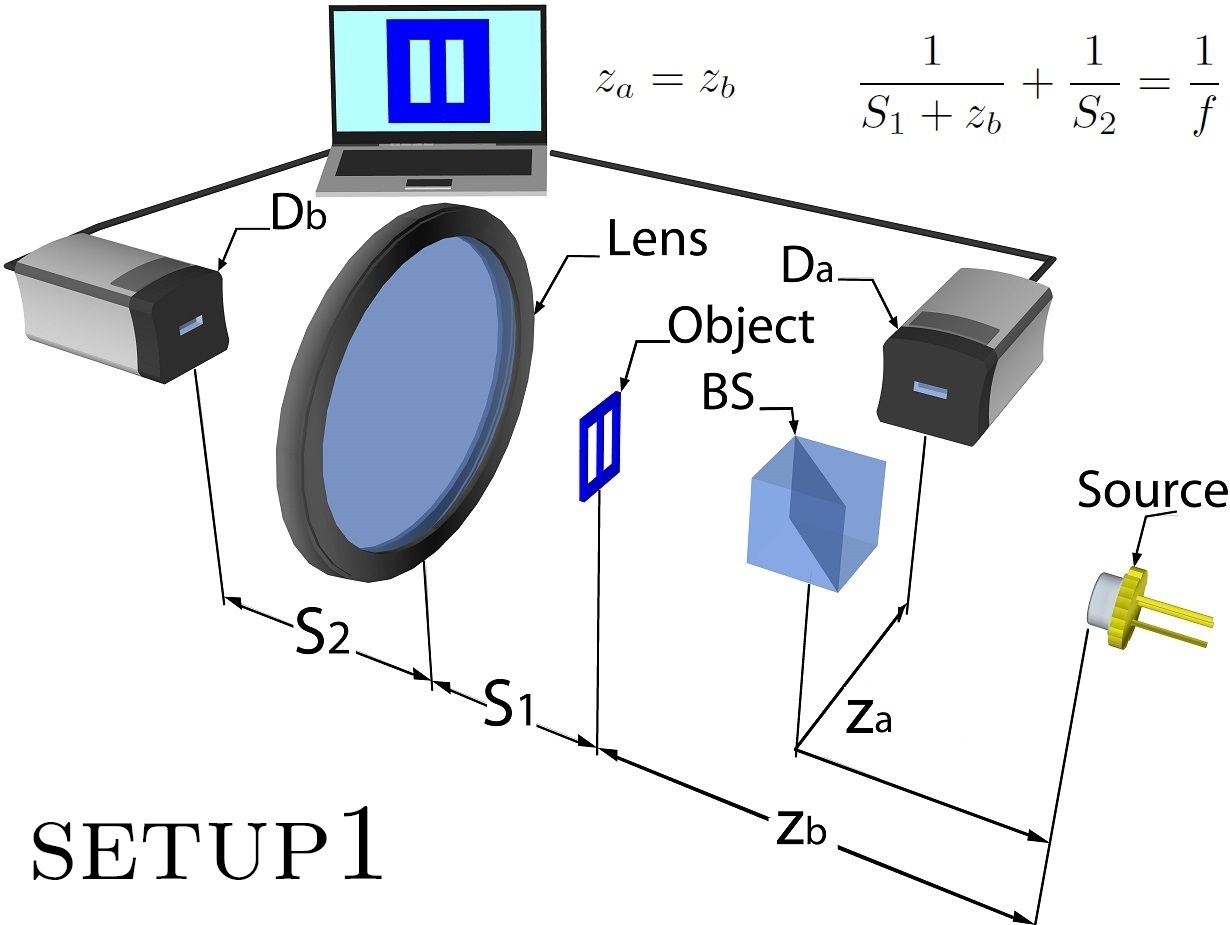 Figure 1
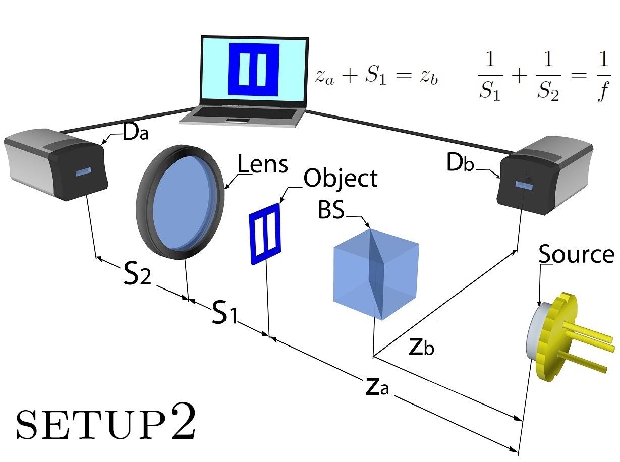 Figure 2
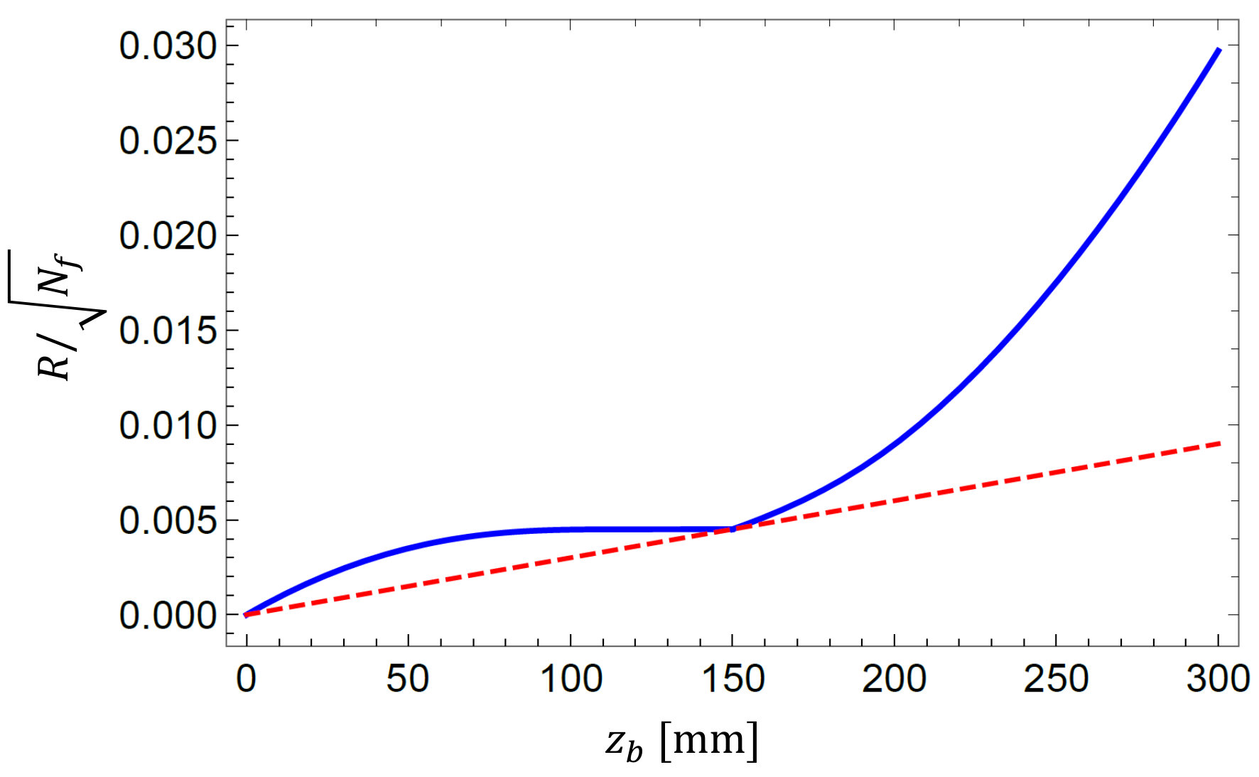 Figure 3
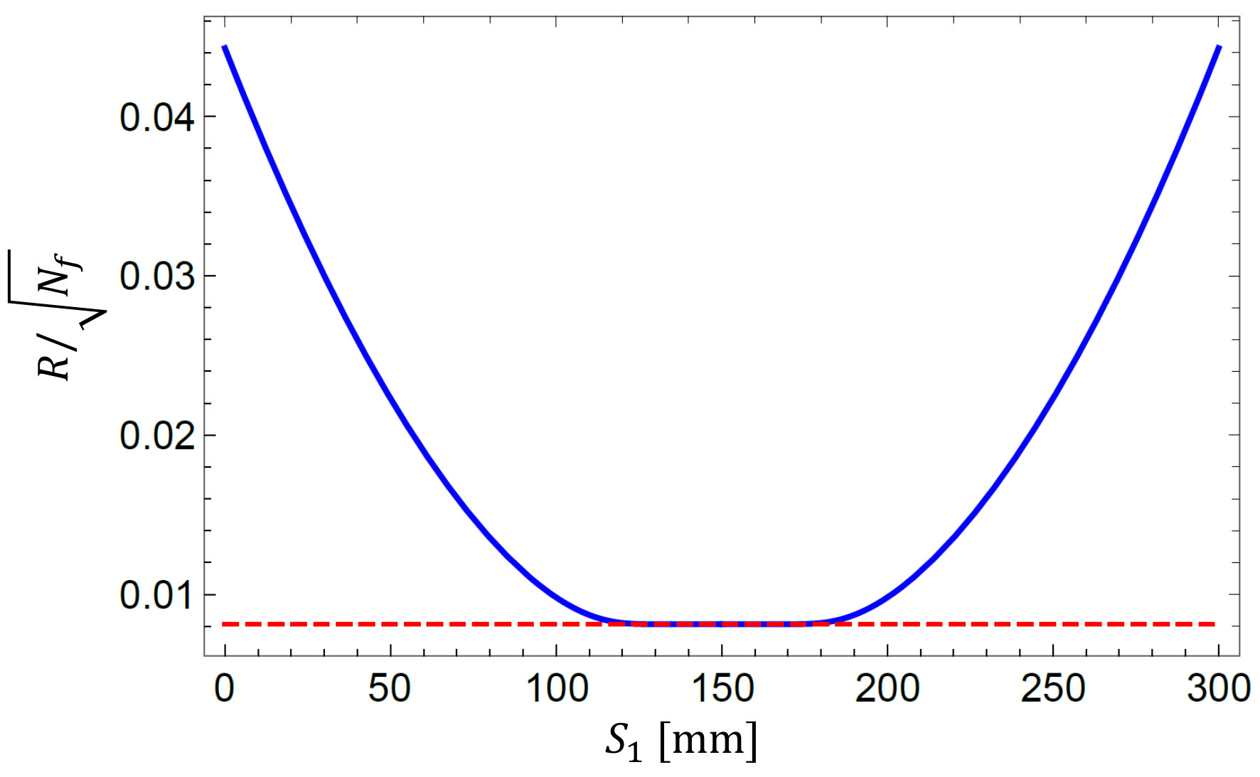 Figure 4
Peer Reviews
No public reviews on file for this paper yet. If you reviewed it on a platform where reviews are public (OpenReview, ICLR, NeurIPS, ICML), you can paste yours below so the community can read it here.
Videos
No videos yet. Explain this paper in a talk, walkthrough, or lecture? Add one.
Signal-to-noise properties of correlation plenoptic imaging with chaotic light
Giovanni Scala
Dipartimento Interateneo di Fisica, Università degli Studi di Bari, I-70126 Bari, Italy
INFN, Sezione di Bari, I-70125 Bari, Italy
Milena D’Angelo
Dipartimento Interateneo di Fisica, Università degli Studi di Bari, I-70126 Bari, Italy
Istituto Nazionale di Ottica (INO-CNR), I-50125 Firenze, Italy
INFN, Sezione di Bari, I-70125 Bari, Italy
Augusto Garuccio
Dipartimento Interateneo di Fisica, Università degli Studi di Bari, I-70126 Bari, Italy
INFN, Sezione di Bari, I-70125 Bari, Italy
Saverio Pascazio
Dipartimento Interateneo di Fisica, Università degli Studi di Bari, I-70126 Bari, Italy
INFN, Sezione di Bari, I-70125 Bari, Italy
Istituto Nazionale di Ottica (INO-CNR), I-50125 Firenze, Italy
Francesco V. Pepe
INFN, Sezione di Bari, I-70125 Bari, Italy
Abstract
Correlation Plenoptic Imaging (CPI) is a novel imaging technique, that exploits the correlations between the intensity fluctuations of light to perform the typical tasks of plenoptic imaging (namely, refocusing out-of-focus parts of the scene, extending the depth of field, and performing 3D reconstruction), without entailing a loss of spatial resolution. Here, we consider two different CPI schemes based on chaotic light, both employing ghost imaging: the first one to image the object, the second one to image the focusing element. We characterize their noise properties in terms of the signal-to-noise ratio (SNR) and compare their performances. We find that the SNR can be significantly higher and easier to control in the second CPI scheme, involving standard imaging of the object; under adequate conditions, this scheme enables reducing by one order of magnitude the number of frames for achieving the same SNR.
I Introduction
Plenoptic imaging is a recently established optical imaging technique, based on the idea of recording both the spatial distribution and propagation direction of light in a single exposure adelson . Although the first feasible proposal to apply plenoptic imaging to digital cameras dates back to the mid-2000s ng , the seminal intuition can be attributed to Lippmann lippmann one century earlier. Plenoptic imaging is currently employed in a very wide range of applications, that include stereoscopy adelson ; muenzel ; levoy , microscopy microscopy1 ; microscopy2 ; microscopy3 ; microscopy4 , particle image velocimetry piv , particle tracking and sizing tracking , and wavefront sensing thesis_wu ; eye ; atmosphere1 ; atmosphere2 . Since plenoptic devices are able to simultaneously acquire 2D images from multiple perspectives, they are considered among the fastest and most promising methods for 3D imaging 3dimaging , as shown by the very recent use in imaging of animal neuronal activity microscopy4 , surgical robotics surgery , endoscopy endoscopy and blood-flow visualization piv2 .
Currently available plenoptic imaging devices are based on the intensity measurement on a single detector ng ; georgiev1 ; georgiev2 . Their key component is a microlens array, that produces multiple images of some reference plane, not coinciding with the object plane defined by the main lens. In this way, the direction of light from the object plane to such reference plane can be traced, enabling to reconstruct (refocus) out-of-focus parts of the scene, extend the depth of field, and perform 3D imaging in post-processing. However, capturing directional information entails a fundamental tradeoff with the image resolution. In particular, spatial resolution in plenoptic devices cannot reach the diffraction limit, as determined by the light wavelength and the numerical aperture of the imaging system.
Several technologies have been developed in the field of quantum imaging, which go beyond the capabilities of standard imaging and interferometry systems pittman ; qu_superres ; qu_superres2 ; sofi ; undetected ; dangelo_kim ; scarcelli_er ; tamma ; genovese_review . Recently, a technique named Correlation Plenoptic Imaging (CPI) cpi_review has been shown to overcome the typical tradeoff between spatial and directional resolution of plenoptic imaging, by exploiting intensity correlations of either chaotic light cpi_prl ; cpi_qmqm ; cpi_jopt ; cpi_exp or entangled photon pairs cpi_technologies . The key idea of CPI is to encode information of the image and the direction of light in two distinct sensors: the desired information emerges by evaluating intensity correlations. Since two separate sensors are used, the image resolution can reach the diffraction limit. CPI is inspired by ghost imaging with chaotic and entangled light pittman ; gatti ; valencia ; scarcelliPRL ; bennink ; devaux ; laserphys ; shapiro_review , with a crucial modification: the “bucket” detector, collecting all light that propagates in one optical path in ghost imaging, is replaced by a spatially resolving detector in CPI. The resolution of such detector enables to track the direction of light.
Though the tradeoff between spatial and directional resolution can be overcome by using CPI instead of traditional plenoptic imaging, the former has the disadvantage of requiring the reconstruction of the source statistics, thus losing the single-shot advantage of standard plenoptic imaging. The signal-to-noise ratio (SNR) improves with the number of frames; however, to aim at performing real-time imaging, the number of acquired frames should be as small as possible. The choice of the optimal frame number is particularly delicate in the case of ghost images with chaotic light, characterized by a well-known tradeoff between resolution and SNR gatti_coh ; erkmen ; osullivan ; brida_pra . Ways to mitigate such tradeoff involve image analysis techniques katz ; welsh and alternative measurement schemes ferri_dgi . The objective of this paper is to characterize and compare the SNR in two different CPI schemes based on the properties of chaotic light and designed according to complementary concepts (see Fig. 1): the first one (setup1) exploits ghost imaging to obtain the image of the object, and standard imaging to get directional information, while in the second one (setup2) the object is imaged by a lens, and ghost imaging is used to obtain directional information.
In Section II, we will outline the problem and define its general aspects. In Section III, we will derive the results that enable one to determine the optimal number of frames to be acquired to achieve the chosen SNR, given the light properties, the optical distances and the object features. The results obtained in the two setups will be compared and interpreted. In Section IV, we will further discuss the perspectives of this research.
II Correlation plenoptic imaging schemes
We will consider the two setups (setup1 and setup2) represented in Fig. 1, for performing correlation plenoptic imaging. These configurations have been proposed in cpi_prl and cpi_jopt , respectively, and an experimental proof of principle of plenoptic imaging and refocusing in setup1 has been performed cpi_exp . The two schemes essentially differ by the way ghost imaging is employed to obtain an image of either the object plane (setup1) or the focusing element (setup2). The common feature of the two setups is the fact that light emitted by a chaotic source is split in two paths and by a beam splitter (BS), and is recorded at the end of each path by the high-resolution detectors and . An object is always placed in one of the two paths. More specifically, intensity patterns and , with the coordinate on each detector plane, are recorded in time to reconstruct the correlation function
[TABLE]
with . The expectation value in (1) must be evaluated over the source statistics, but it can be approximated by the time average of the product of the intensity fluctuations, provided the source is stationary and ergodic mandel . In the discussed setups, the images of the object plane and of the focusing element aperture will be simultaneously encoded in .
In setup1, an image of the object can be obtained only by measuring intensity correlations between and . Along path (the reflected path in figure), light directly impinges on detector , placed at an optical distance from the source. In path (the transmitted path in figure), a transmissive object lies at a distance from the source. A thin lens of focal length is placed between the object and the detector , at a distance from the former and from the latter. Such distances are chosen in order to focus the source on with magnification , hence, they satisfy the thin-lens equation . In the case , measurement of the correlation function and direct integration over provides the focused ghost image of the object scarcelliPRL .
In setup2, the image of the lens is recovered from intensity correlations between and . Along path (the reflected path in figure), light directly impinges on the detector , placed at an optical distance from the source. In path (the transmitted path in figure), the transmissive object is placed at a distance from the source. The thin lens of focal length lies between the object and the detector , at a distance from the former and from the latter. In this case, the setup is designed to obtain a focused ghost image of the lens on the detector : therefore, distances are fixed in order to satisfy . The object-to-lens and lens-to- distances are arbitrary. However, it is intuitive that, if , such that , the image of the object will be sharply focused on .
The refocusing capability of both setups is determined by the fact that the correlation function (1) encodes multiple coherent images of the object, one for each point on . The images corresponding to different pixels on are generally displaced with respect to each other, unless a focusing condition is satisfied. In the focused case, integration over detector yields an incoherent image. In the out-of-focus cases, the collected coherent images need to be realigned before integrating over , following
[TABLE]
with
[TABLE]
The parameters , that approach at focus, are properly chosen to realign the coherent images depending on the setup, and read
[TABLE]
It is evident that, when the focusing conditions are fulfilled, there is no need to shift and rescale the first argument of , and the high resolution of detector plays no role. In all other cases, the spatial resolution of is essential to reconstruct the image of an out-of-focus object, which, by direct integration over , would appear blurred and degraded.
III Fluctuations and SNR
III.1 General aspects and statistical model
The objective of this paper is to estimate the signal-to-noise ratio characterizing the refocused images retrieved in setup1 and setup2. To this end, we shall analyze the fluctuations of the refocused observable , defined in Eq. (3), around its average , namely
[TABLE]
with determined by the local fluctuations of the intensity correlations [see Eq. (3)]. Let us assume that frames are collected in time to evaluate the expectation value (2). Supposing their statistical independence, the root-mean-square error affecting the evaluation of can be estimated by . We therefore define the quantity
[TABLE]
as the signal-to-noise ratio.
A scalar model of the electromagnetic field, in which the effects of polarization are neglected, will be adopted, and we will assume that the radiation emission by the source is an approximately Gaussian random process, stationary and ergodic. In particular, the field at a point on the source will be characterized by a Gaussian-Schell equal-time correlator mandel
[TABLE]
with the peak intensity, the width of the intensity profile , and the transverse coherence length on the source plane. Since we are interested in chaotic sources, characterized by negligible transverse coherence, we will also approximate the mutual coherence function with a delta function
[TABLE]
under the integrals.
To compute (2) and (III.1), it is necessary to determine up to eight-point field correlators. Using the Gaussian approximation, we will assume that Isserlis-Wick’s theorem isserlis is valid for the correlators that involve an equal number of ’s and ’s, namely
[TABLE]
with a permutation of the primed indexes, while all other expectation values, including and , vanish. Propagation from the source to the detectors along the two paths and is deterministic, and depends on the transmission functions of the object and the lens. Concerning propagation in free space, a monochromatic field with frequency and wavenumber , evaluated on a plane at a general longitudinal position , is related to the field at by the paraxial transfer function goodman :
[TABLE]
The correlators between fields and at the detectors and , that determine the refocused image and the fluctuation , thus inherit the factorization property (9) from the fields on the source. In particular, since and , the correlation of intensity fluctuations between the two detectors, defined in Eq. (1), reads
[TABLE]
Computation of the fluctuation (III.1), based on the definition (3), also involves the autocorrelations of intensity fluctuations at the same detector,
[TABLE]
with .
In both setups, is determined with good approximation by the contribution that features only the autocorrelations:
[TABLE]
Other contributions are typically suppressed as
[TABLE]
with the number of transverse modes that propagate towards the detector . Therefore, in the following, we shall approximate when computing the SNR. However, the full computation of all contributions to is presented in the Appendix.
III.2 Analysis of setup1
Let us first consider setup1 (Fig. 1, upper panel). Let us call the aperture function of the transmissive object, and neglect the finite pupil size of the lens, by assuming that it does not affect propagation along path . Combining free propagation (10) with transmission through the object and the lens goodman , and applying the statistical assumptions (7)-(8)-(9) on the field correlations at the source, we obtain the correlation between the fluctuations of the intensities and , which reads
[TABLE]
with as in (4), and the coefficients
[TABLE]
while , with
[TABLE]
Since is a generally complex quantity, it will be useful in the following to split it into its real and imaginary parts as . The result (III.2) shows that, by varying , a collection of coherent images of the object is obtained on .
Combining Eq. (III.2) with the definitions (2)–(4), we determine the refocused image
[TABLE]
with
[TABLE]
and . This quantity is regular in the focused limit , where the -dependent part of the integral takes the form
[TABLE]
which is exactly the unit-magnification incoherent image obtained in the case of lensless ghost imaging scarcelliPRL ; osullivan , whose point-spread function is determined by the squared Fourier transform of the source intensity profile. In the geometrical optics limit (), the dominant contribution to the integral (III.2) comes from the stationary point of the real and imaginary parts of the exponent, yielding
[TABLE]
which also shows that actually provides a refocused image of the object, characterized by unit magnification.
Let us now evaluate the autocorrelations of the intensity fluctuations
[TABLE]
where
[TABLE]
with , is the transverse coherence length on the planes at a distance from the source. The correlation functions (22)-(23) enable to evaluate the dominant contribution to the variance of the correlation of the intensity fluctuations in Eq. (III.1), that reads
[TABLE]
with
[TABLE]
The most relevant (and interesting) feature of such quantity is its independence on the coordinate on . Therefore, the signal is noisy and superposed to a further background noise. Such constant background noise stems from the fact that the intensity profile of the light impinging on is, in the case of setup1, not related to the spatial profile of the signal : actually, as one can easily check, the intensity profile on is approximately uniform, and carries no information on the object transmission function .
At this point, the SNR can be exactly evaluated, as a function of the number of collected frames, by using the results (18)-(25) in the expression (6). A useful and intuitive estimate is given by the geometrical-optics approximation of , which reads
[TABLE]
with
[TABLE]
Let us first discuss this result in the focused case, in which and . The integrand of (28) becomes localized around , and the value of the SNR reduces to
[TABLE]
The above expression highlights the dependence of the SNR on the ratio between the coherence area on the object and an “effective area” of the object itself, given by the integral of the factor, which is equal to the actual area in the case of binary transmission function. Since the same coherence area determines the resolution through (20), this result entails the well-known tradeoff between resolution and SNR typical of ghost imaging gatti_coh ; erkmen ; brida_pra ; osullivan .
Deep in the out-of-focus regime, when becomes larger than the typical size of the object, the exponential modulation under the integral (28) can be neglected, yielding
[TABLE]
with the light wavelength. This expression shows a less trivial dependence on the longitudinal position of the refocused plane, but can still be interpreted in terms of the resolution-SNR tradeoff. Actually, as discussed in cpi_prl ; cpi_exp , a good estimate of the resolution of the refocused image is given by , where is the typical linear size of the smallest transmissive parts of the object. Notice, however, that the inverse dependence on the effective area of the object has changed with respect to the focused case(29). As a rule of thumb, we can estimate the SNR of refocused images as
[TABLE]
a result that depends on the product of the ratios (resolution cell)/(total area) and (smallest detail area)/(total area). In Fig. 2, we show the behavior of the SNR in setup1 as a function of the source-to-object distance , comparing the result with the case of a focused ghost image taken with [Eq. (29)]. The higher SNR of correlation plenoptic imaging is related to the lower resolution of the refocused image with respect to the focused ghost image.
III.3 Analysis of setup2
In the analysis of setup2, we shall consider a finite-size pupil of the lens, that determines the spatial resolution, and assume that the transverse size of the source is asymptotically large, namely, that the finite size of the source does not affect in a relevant way the correlation of the intensity fluctuations. In this way, the most relevant part of the mutual correlation function reads
[TABLE]
where
[TABLE]
which coincides with the Fourier transform of the pupil function, represents the coherent PSF of the focused image (obtained when and ), and , with
[TABLE]
The refocused image, defined by in Eq. (4) (second formula), reads
[TABLE]
with
[TABLE]
One can easily check that, in the focused case , the above expression reduces to the incoherent image of the transmission function of the object, whose point-spread function is related to the usual square modulus of the Fourier transform of the lens pupil function . In the general case, the plenoptic imaging property emerges when considering the geometrical optics limit, in which the complicated expression (35) simplifies to
[TABLE]
where is the absolute magnification provided by the lens, and is the (effective) area of the lens.
The autocorrelations, computed in the same regime of large source width , read
[TABLE]
Notice that the autocorrelation on the detector diverges with increasing : therefore, even if the finite size of the source can become irrelevant for the average correlation of intensity fluctuations, the variance of this quantity crucially depends on it.
Also in this case, the dominant contribution to the variance of can be evaluated by considering the autocorrelations. However, the computation of (III.1) must take into account the finite size of the detector , since, integrating without bounds on would yield a divergent result. Since the role of is to detect the ghost image of the lens, which is characterized by unit magnification, the optimal size of this detector is given by the size of the lens. Following these considerations and the result (38), valid in the limit of large source width , one obtains
[TABLE]
In the focused case, the integral in (III.3) is trivially proportional to , which is -dependent, as opposed to the case of setup1. In the general case, the analytic evaluation of (III.3) can become impossible when considering the actual detector area as the integration domain. However, one can perform the computation by regularizing the integral with a Gaussian envelope function , where is the area of detector (or, better, the area of the part of the detector that accommodates the image of the lens).
The geometrical-optics approximation of (III.3) reads
[TABLE]
with
[TABLE]
The spatial behavior of the variance is now much less trivial than the constant behavior found in setup1. Actually, in the focused limit , the integrand of (III.3) becomes infinitely localized around , leading to . This means that, at least in the focused case, noise is proportional to the signal. Such feature is related to the fact that, in this case, the field transmitted by the object is focused on , and this is reflected in all the correlation functions involving . This feature is absent in the focused case of setup1, in which the field impinging on extends well beyond the shape of the object, and the image emerges only from intensity correlation measurements. In the opposite limit of large defocusing, instead, the spatial dependence of the lens pupil function under the integral (III.3) becomes irrelevant, and the result implies that the measurement of comes with a uniform background noise. However, as we shall presently find, such background is more easily controllable than the one surrounding the ghost image in setup1.
Based on the above considerations, the estimate of the SNR based on Eq. (6) is less trivial than in setup1, since the denominator depends on and shows different spatial behaviors with varying defocusing. The geometrical-optics expression of the SNR reads
[TABLE]
In the focused case, the above quantity reduces to the simple expression
[TABLE]
a result that does not depend on , since noise is proportional to the signal. The constant SNR in (44) is essentially the square root of the ratio of the coherence area on and the area of the same detector, which can also be interpreted as (coherence area on the lens)/(area of the lens), in perfect analogy with Eq. (29), after replacing the object with the lens. The SNR thus coincides with the one expected for the ghost image of the lens.
In the out-of-focus case, a background noise emerges, and the SNR becomes similar in form to (30), yielding
[TABLE]
The ratio between the area of the lens and the area of the object is generally large for image magnification , and the SNR also increases quadratically with defocusing, providing a generally more favorable picture compared to setup1. A good rule to estimate the order of magnitude of the refocused image SNR thus reads
[TABLE]
where we have assumed that the area of the detector is matched to the area of the lens. In Fig. 3, we represent the behavior of the SNR in setup2 as a function of the object-to-lens distance , and compare the result with the case of a focused image taken with (notice that is a function of ).
III.4 Summary of the results
We have discussed the properties of the signal-to-noise ratio for setup1 and setup2, finding that the results obtained for the latter are generally more advantageous than for the former. In the focused case, setup2 is characterized by the suppression of background noise, that, on the other hand, is a typical feature affecting the ghost image obtained in setup1. Moreover, noise in setup1 increases with improving resolution on the object, thus entailing a trade-off between resolution and SNR trade-off. In the out-of-focus case, background noise is present in both configurations. However, in setup1 it depends on small quantities, namely the ratios between the area of an effective resolution cell and the total area of the object, and , where the numerator is the area corresponding to the size of the finest details of the object. In setup2, instead, we find that the SNR depends also on the ratio , a quantity that is not necessarily small. Therefore, we expect that a smaller number of frames is needed to achieve the same resolution in setup2 compared to setup1.
To get a quantitative hint of the SNR improvement in setup2, we compare the results shown in Figs. 2-3, which are referred to two cases that are as homogeneous as possible in terms of resolution, depth of field and magnification of the focused image. We find that he ratio between the SNR in setup2 and setup1 at fixed is consistently larger than one: when such a ratio reaches values around , for an object placed at , one tenth of the frames is needed in setup2 to reach the same SNR as in setup1. Notice that, by considering the expressions (30)-(III.3), the ratio of the SNRs for out-of-focus images is very weakly dependent of the light wavelength and the area of the object, provided the conditions for the validity of geometrical optics approximation are satisfied.
IV Conclusions and outlook
Performing plenoptic imaging by correlation measurements has the potential to improve 3D imaging and microscopy, since it combines high resolution with the possibility to gain directional information. The results obtained in this Article provide the experimenter with rules to determine the scaling of the SNR with the number of frames, and consequently to fix the number of frames needed for a fast and accurate imaging of the scene. The problem of optimizing the acquisition time is particularly relevant both in view of real-time imaging and in all those cases in which additional difficulties in retrieving intensity correlations are present, as it happens when considering unconventional sources like X rays pelliccia ; schneider to perform CPI. In our future research, we plan to extend our analysis to the case in which CPI is performed with entangled photons cpi_technologies , investigating whether the remarkable results observed in other kinds of imaging schemes brida_nat ; meda ; samantaray , in which the shot-noise limit can be overcome, would yield analogous improvements in a setup oriented to plenoptic imaging.
Acknowledgments
MD, AG and FVP are supported by Istituto Nazionale di Fisica Nucleare (INFN) through the project “PICS”. MD, AG, SP and GS are supported by Istituto Nazionale di Fisica Nucleare (INFN) through the project “QUANTUM”. AG and MD are supported by the Italian Ministry of Education, University and Research (MIUR) through project PON Ricerca e Innovazione ARS01_00141.
Appendix A
We have identified and discussed the term , defined in Eq. (III.1), as the most relevant term to determine the SNR in both setups. Here, we provide the computation of the remaining terms characterizing the local fluctuations :
[TABLE]
that characterize the variance at a point , in the geometrical-optics approximation. In (47), all but one term are conjugate to each other, namely with . The independent contributions read
[TABLE]
and
[TABLE]
Notice that, in the focused case, both and exactly reduce to the squared refocus image , defined in Eq. (2).
A.1 Results for setup1
The term reads
[TABLE]
with
[TABLE]
where , , and are defined in Eqs. (16)-(17), and
[TABLE]
[TABLE]
The functions and in (54) are defined as follows:
[TABLE]
In the geometrical optics limit, the function in (51) reduces to
[TABLE]
The term reads
[TABLE]
with
[TABLE]
and defined in Eq. (A.1), while the argument of the exponential reads
[TABLE]
with [see Eq. (55)]
[TABLE]
The geometrical optics result
[TABLE]
The terms and in Eq. (A) are both complex and very similar to each other. In this case,
[TABLE]
with
[TABLE]
where
[TABLE]
coincides, for an object characterized by a real transmission function, with defined in Eq. (A.1), and
[TABLE]
with
[TABLE]
The coefficients and appearing in Eq. (67) are defined as
[TABLE]
In the geometrical optics limit, and approach the same value, namely
[TABLE]
where
[TABLE]
A.2 Results for setup2
As in the main text, we will consider a lens with a finite pupil function and an asymptotically large source. The term , as defined in (48), reads
[TABLE]
with
[TABLE]
with as defined in Eq. (34), , and
[TABLE]
The stationary-phase approximation provides the result
[TABLE]
with .
The result for is
[TABLE]
with
[TABLE]
where
[TABLE]
The geometrical optics approximation of (78) reads
[TABLE]
Let us finally compute the remaining independent terms and . Since, after the assumption of asymptotically large source, , the two terms are incidentally equal to each other, and read
[TABLE]
with
[TABLE]
with defined in Eq. (76) and
[TABLE]
The geometrical optics limit yields
[TABLE]
The reference list from the paper itself. Each links out to its DOI / PubMed record.
- 1(1) E. H. Adelson and J. Y. Wang, “Single lens stereo with a plenoptic camera,” IEEE Trans. Pattern Anal. Mach. Intell. 14 , 99 (1992).
- 2(2) R. Ng, M. Levoy, M. Brédif, G. Duval, M. Horowitz, and P. Hanrahan, “Light field photography with a hand-held plenoptic camera,” Stanford University Computer Science Tech Report CSTR 2005-02, 2005.
- 3(3) G. Lippmann, “Épreuves réversibles donnant la sensation du relief,” J. Phys. Theor. Appl. 7 , 821 (1908).
- 4(4) S. Muenzel and J. W. Fleischer, “Enhancing layered 3d displays with a lens,” Appl. Opt. 52 , D 97 (2013).
- 5(5) M. Levoy and P. Hanrahan, “Light field rendering,” in Proceedings of the 23rd Annual Conference on Computer Graphics and Interactive Techniques (Association for Computing Machinery, New York, 1996), pp. 31–42.
- 6(6) M. Levoy, R. Ng, A. Adams, M. Footer, and M. Horowitz, “Light field microscopy,” ACM Trans. Graph. 25 , 924 (2006).
- 7(7) M. Broxton, L. Grosenick, S. Yang, N. Cohen, A. Andalman, K. Deisseroth, and M. Levoy, “Wave optics theory and 3-d deconvolution for the light field microscope,” Opt. Express 21 , 25418 (2013).
- 8(8) W. Glastre, O. Hugon, O. Jacquin, H. G. de Chatellus, and E. Lacot, “Demonstration of a plenoptic microscope based on laser optical feedback imaging,” Opt. Express 21 , 7294 (2013).