The First NuSTAR Observation of 4U 1538-522: Updated Orbital Ephemeris and A Strengthened Case for an Evolving Cyclotron Line Energy
Paul B. Hemphill (1), Richard E. Rothschild (2), Diana M. Cheatham (3, and 4), Felix F\"urst (5), Peter Kretschmar (5), Matthias K\"uhnel (6), Katja, Pottschmidt (3, 4), R\"udiger Staubert (7), J\"orn Wilms (6), Michael T., Wolff (8) ((1) MIT Kavli Institute

TL;DR
This study presents the first NuSTAR observations of 4U 1538-522, updating its orbital parameters and providing evidence for the secular evolution of its cyclotron line energy, with detailed spectral and timing analysis during eclipse phases.
Contribution
It offers the first NuSTAR spectral and timing analysis of 4U 1538-522, updating orbital parameters and strengthening evidence for evolving cyclotron line energy.
Findings
Marginal orbital period evolution detected.
Cyclotron line energy increased since previous measurements.
Characterized iron line behavior during eclipse ingress and egress.
Abstract
We have performed a comprehensive spectral and timing analysis of the first NuSTAR observation of the high-mass X-ray binary 4U 1538-522. The observation covers the X-ray eclipse of the source, plus the eclipse ingress and egress. We use the new measurement of the mid-eclipse time to update the orbital parameters of the system and find marginally-significant evolution in the orbital period, with yr. The cyclotron line energy is found approximately 1.2 keV higher than RXTE measurements from 1997--2003, in line with the increased energy observed by Suzaku in 2012 and strengthening the case for secular evolution of 4U 1538-522's CRSF. We additionally characterize the behavior of the iron fluorescence and emission lines and line-of-sight absorption as the source moves into and out of eclipse.
Click any figure to enlarge with its caption.
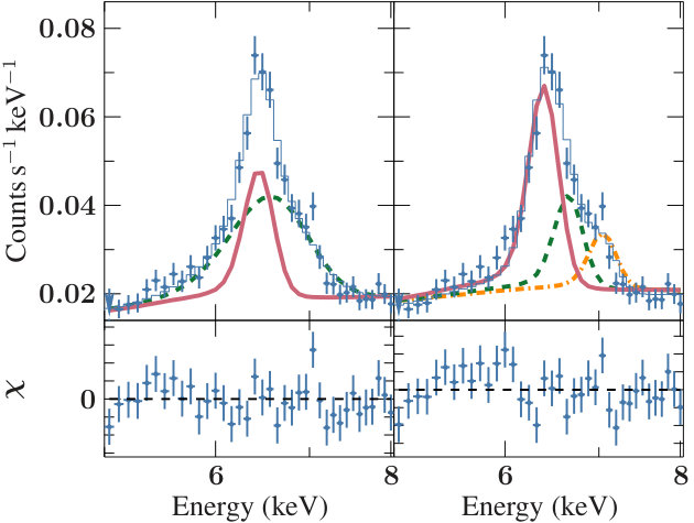 Figure 1
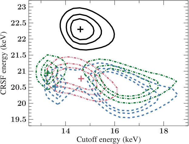 Figure 2
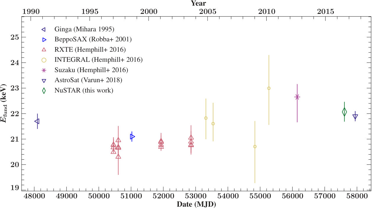 Figure 3
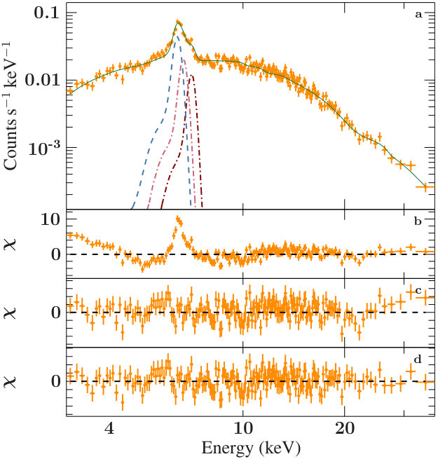 Figure 4
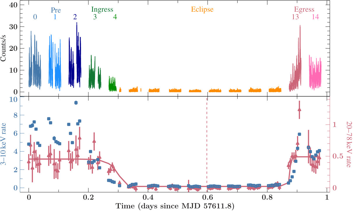 Figure 5
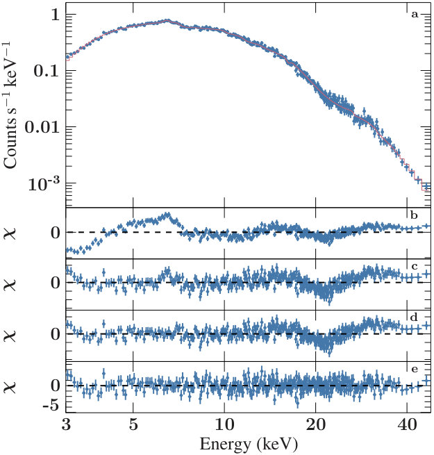 Figure 6
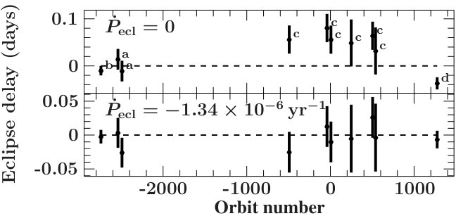 Figure 7
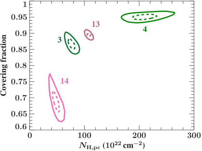 Figure 8
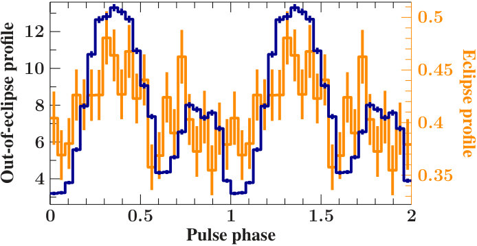 Figure 9
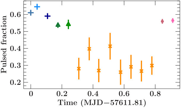 Figure 10
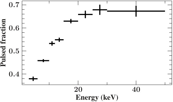 Figure 11
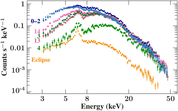 Figure 12
| Phase | Days | |
|---|---|---|
| MJD | ||
| d | ||
| MJD | ||
| d | ||
| Eclipse duration | d | |
| MJD |
| Parameter | Value |
|---|---|
| (d) | 3.728354(9) |
| ( yr-1) | |
| (d) | 3.72831(2) |
| ( yr-1) | |
| (MJD) | |
| (lt-s) | **From Mukherjee et al. (2006) and Falanga et al. (2015). |
| (degrees) | ††For the indicated , extrapolated using Falanga et al. (2015)’s measurement of deg yr-1. |
| (deg yr-1) | **From Mukherjee et al. (2006) and Falanga et al. (2015). |
| Eccentricity | 0.18(1)**From Mukherjee et al. (2006) and Falanga et al. (2015). |
| (s) |
| mplcut | fdco | npex | ||||
|---|---|---|---|---|---|---|
| FluxaaUnabsorbed flux in 3–50 keV band. ( erg cm-2 s-1) | ||||||
| ( cm-2) | ||||||
| (keV) | ||||||
| (keV) | ||||||
| Smoothing area ( ph cm-2 s-1) | ||||||
| ( ph cm-2 s-1) | ||||||
| (keV) | ||||||
| (keV) | ||||||
| (keV) | ||||||
| (keV) | ||||||
| (keV) | ||||||
| (keV) | ||||||
| Fe KccK and 7 keV line widths fixed to 0.01 keV. area ( ph cm-2 s-1) | ||||||
| Fe K energy (keV) | ||||||
| 7 keV line area ( ph cm-2 s-1) | ||||||
| 7 keV line energy (keV) | ||||||
| 0.99 (630) | 1.08 (633) | 1.01 (631) |
| Ingress | Eclipse | Egress | |||
|---|---|---|---|---|---|
| 3 | 4 | 5–12 | 13 | 14 | |
| FluxaaUnabsorbed flux in 3–50 keV band. ( erg cm-2 s-1) | |||||
| bbValues in parentheses were frozen during fitting. ( cm-2) | ccValues in parentheses were frozen during fitting. | ||||
| ( cm-2) | |||||
| (keV) | |||||
| (keV) | |||||
| (keV) | |||||
| (keV) | |||||
| (keV) | |||||
| Fe K energyddFe K, K, and Fe XXV line widths fixed to 0.01 keV. (keV) | |||||
| Fe K area ( ph cm-2 s-1) | |||||
| Fe K EW (eV) | |||||
| Fe XXV energy (keV) | |||||
| Fe XXV area ( ph cm-2 s-1) | |||||
| Fe XXV EW (eV) | |||||
| Fe K energy (keV) | |||||
| Fe K area ( ph cm-2 s-1) | |||||
| Fe K EW (eV) | |||||
| 1.08 (438) | 0.92 (288) | 1.10 (362) | 0.99 (518) | 1.01 (474) | |
Peer Reviews
No public reviews on file for this paper yet. If you reviewed it on a platform where reviews are public (OpenReview, ICLR, NeurIPS, ICML), you can paste yours below so the community can read it here.
Videos
No videos yet. Explain this paper in a talk, walkthrough, or lecture? Add one.
The First NuSTAR Observation of 4U 1538522: Updated Orbital Ephemeris and A Strengthened Case for an Evolving Cyclotron Line Energy
Kavli Institute for Astrophysics and Space Research, Massachusetts Institute of Technology, Cambridge, MA 02139, USA
Richard E. Rothschild
Center for Astrophysics and Space Sciences, University of California, San Diego, 9500 Gilman Dr., La Jolla, CA 920093-0424, USA
Diana M. Cheatham
Center for Space Science and Technology, University of Maryland Baltimore County, 1000 Hilltop Circle, Baltimore, MD 21250, USA
CRESST and NASA Goddard Space Flight Center, Astrophysics Science Division, Code 661, Greenbelt, MD 20771, USA
Felix Fürst
European Space Astronomy Centre (ESAC), Science Operations Departement, 28692 Villanueva de la Cañada, Madrid, Spain
Peter Kretschmar
European Space Astronomy Centre (ESAC), Science Operations Departement, 28692 Villanueva de la Cañada, Madrid, Spain
Matthias Kühnel
Dr. Karl Remeis-Sternwarte & Erlangen Center for Astroparticle Physics, Sternwartstr. 7, 96049 Bamberg, Germany
Katja Pottschmidt
Center for Space Science and Technology, University of Maryland Baltimore County, 1000 Hilltop Circle, Baltimore, MD 21250, USA
CRESST and NASA Goddard Space Flight Center, Astrophysics Science Division, Code 661, Greenbelt, MD 20771, USA
Rüdiger Staubert
Institut für Astronomie und Astrophysik, Universität Tübingen, Sand 1, 72076 Tübingen, Germany
Jörn Wilms
Dr. Karl Remeis-Sternwarte & Erlangen Center for Astroparticle Physics, Sternwartstr. 7, 96049 Bamberg, Germany
Michael T. Wolff
Space Science Division, Naval Research Laboratory, Washington, DC 20375-5352, US
Abstract
We have performed a comprehensive spectral and timing analysis of the first NuSTAR observation of the high-mass X-ray binary 4U 1538522. The observation covers the X-ray eclipse of the source, plus the eclipse ingress and egress. We use the new measurement of the mid-eclipse time to update the orbital parameters of the system and find marginally-significant evolution in the orbital period, with yr*-1*. The cyclotron line energy is found approximately 1.2 keV higher than RXTE measurements from 1997–2003, in line with the increased energy observed by Suzaku in 2012 and strengthening the case for secular evolution of 4U 1538522’s CRSF. We additionally characterize the behavior of the iron fluorescence and emission lines and line-of-sight absorption as the source moves into and out of eclipse.
X-rays: individual (4U 1538522 (catalog 4U 1538-522)) — stars: individual (QV Nor (catalog )) — stars: magnetic field — X-rays: binaries — binaries: eclipsing — accretion
††facilities: NuSTAR††software: ISIS (Houck & Denicola, 2000), HEASOFT, Mathematica
\AuthorCallLimit
=20
1 Introduction
High-mass X-ray binaries (HMXBs) present interesting laboratories for a number of astrophysical questions. As endpoints of stellar evolution, they provide lever arms on models for stellar and binary evolution, and their high accretion rates and strong magnetic fields (in HMXBs hosting neutron stars) allow us to probe areas of plasma physics inaccessible to terrestrial laboratories. The eclipsing X-ray pulsar 4U 1538522 has been an interesting source in both of these regards since its discovery by Uhuru in the 1970s (Giacconi et al., 1974). Uhuru established the eclipsing nature of the source (see, e.g., Cominsky & Moraes, 1991), while X-ray pulsations were discovered by Davison et al. (1977) and Becker et al. (1977). The pulsar is slow-spinning, with a pulse period of 526.5 s, and is currently spinning down at a rate of 0.1 s yr*-1* as revealed by Fermi/GBM111See http://gammaray.nsstc.nasa.gov/gbm/science/pulsars (Finger et al., 2009). The distance is somewhere in the neighborhood of 6.5 kpc (see, e.g., Crampton et al., 1978; Ilovaisky et al., 1979; Reynolds et al., 1992; Clark, 2004); Gaia parallax measurements (Bailer-Jones et al., 2018) place the source at kpc. In this work we adopt the 6.4 kpc distance measured by Reynolds et al. (1992), as we have in previous work on this source. The X-ray pulsar accretes from the stellar wind of the B0Iab supergiant QV Nor (Reynolds et al., 1992), which it orbits every 3.73 d with regular eclipses (Clark, 2000; Mukherjee et al., 2006; Baykal et al., 2006; Falanga et al., 2015). The neutron star appears to be very low-mass, at 1 (Rawls et al., 2011; Falanga et al., 2015). Despite the eclipsing nature of the source, the binary orbit has historically been difficult to nail down. The orbit is probably eccentric, at (Clark, 2000; Mukherjee et al., 2006), although Clark (2000) and Baykal et al. (2006) also address the circular case, and Rawls et al. (2011) reported difficulty reconciling the observed eclipse duration with an eccentric orbit. The source also may exhibit apsidal advance, as reported by Falanga et al. (2015), although at yr*-1* this is poorly constrained.
In the area of strong magnetic fields and accretion physics, 4U 1538522 is notable for having a cyclotron resonance scattering feature (CRSF, or “cyclotron line”) in its X-ray spectrum, at 22 keV. These pseudo-absorption features arise due to the quantization of cyclotron motion for electrons in strong magnetic fields, which leads to a scattering cross section for photons that is strongly dependent on energy, direction, and polarization. These features provide the only direct measurement of the magnetic field of a neutron star (although it should be noted that this measures a local field strength, compared to more global measurements from, e.g., radio pulsar spin-down). Approximately three dozen sources now have established cyclotron lines, starting with the first discovered in Her X-1 by Trümper et al. (1978). The recent review by Staubert et al. (2018) provides an excellent overview of the current state of the art in cyclotron line studies.
A great deal of work in the past decade has been concerned with the variability of cyclotron lines, mostly in terms of the line energy’s relation to the X-ray luminosity of the source. The basic picture until a few years ago was that sources at very high luminosities exhibited an anti-correlation between CRSF energy and luminosity (see the case of V 0332+53 by Tsygankov et al., 2010), while lower-luminosity sources displayed a positive correlation or no correlation (see, e.g., Staubert et al., 2007; Yamamoto et al., 2011; Klochkov et al., 2012; Müller et al., 2013; Hemphill et al., 2013; Fürst et al., 2014; Hemphill et al., 2016; Doroshenko et al., 2017). Many sources also display considerable variability of the CRSF with pulse phase (see, e.g., Hemphill et al., 2014). Some sources display more complex behavior, such as different variability depending on timescale (e.g., A 0535+26; see Caballero et al., 2008), or possibly dependence on super-orbital variability (e.g., Her X-1; see Staubert et al., 2014). Neutron stars at high accretion rates present a set of incredibly difficult theoretical problems, and their response to changes in accretion rate, as well as the basic question of where cyclotron lines form in the first place, has been a matter of some debate (see, e.g., Becker et al., 2012; Poutanen et al., 2013; Mushtukov et al., 2015a, b; Nishimura, 2015; Schwarm et al., 2017a, b).
This already-difficult problem has been complicated in recent years by the observation of significant secular changes in cyclotron line energies independent of luminosity. The first-discovered instance of a secular change in CRSF energy was Her X-1, when Staubert et al. (2014) reported the discovery of a long-term decay in the line energy over the previous two decades. This trend continued for the next few years (Staubert et al., 2016), but recently, Staubert et al. (2017) have presented evidence that the trend has reversed. La Parola et al. (2016) have argued that a similar decay in CRSF energy is present in Vela X-1, based on Swift/BAT observations. Finally, the BeXRB V 0332+53 displayed hysteresis in its CRSF evolution over the course of its 2015 giant outburst (despite there being no sign of this behavior during its 2003–2004 outburst), with a markedly lower CRSF energy at the end of the outburst compared to the beginning (Cusumano et al., 2016); furthermore, the CRSF energy seems to have rebounded back to its pre-outburst state by the time of its 2016 outburst (Doroshenko et al., 2017; Vybornov et al., 2018).
4U 1538522 is the fourth source in this regard. Its CRSF was originally discovered by Clark et al. (1990) in Ginga observations, analyzed further by Mihara (1995), at 20 keV. In Hemphill et al. (2016), we carried out an extensive re-analysis of the available RXTE, INTEGRAL, and Suzaku data, concluding that there was evidence that the CRSF energy had increased by 1.5 keV between the RXTE observations of the early 2000s and the 2012 Suzaku observation. A recent study of AstroSat data by Varun et al. (2018) has also observed an increased CRSF energy. This rise in energy runs opposite to the long-term secular decays observed in Her X-1 and Vela X-1. It also differs from the outburst-to-outburst increase in CRSF energy observed in V 0332+53 — in 4U 1538522, the change in CRSF energy does not appear to be associated with any major changes in accretion rate, and operates on a timescale of decades, compared to the 1 yr timescale in V 0332+53. 4U 1538522’s CRSF also displays no detected correlation with luminosity (Hemphill et al., 2016), unlike the other sources with detected secular trends.
In this paper we examine our 2016 NuSTAR observation of 4U 1538522 in detail. Section 2 summarizes the observation and data reduction. In Section 3 we present an updated orbital ephemeris based on the new mid-eclipse time. Sections 4.1 and 4.2 summarize the analyses of the pre-eclipse and eclipse portions of the observation. Section 5 discusses these results in the context of past studies of this source and neutron star HMXBs in general.
2 Observations and data reduction
NuSTAR (Harrison et al., 2013) observed 4U 1538522 on 11 August, 2016 for a total exposure of 43.8 ks. The full length of the observation is 84.7 ks, and it covers the eclipse ingress, the eclipse, and the eclipse egress. Based on our ephemeris and mid-eclipse time found in Section 3, and placing phase 0 at the mid-eclipse, the observation covers orbital phases 0.84–0.1, with the eclipse extending 0.07–0.08 in orbital phase to either side of the eclipse center.
We extracted barycentered lightcurves and spectra using the standard NuSTAR pipeline in HEASOFT v6.22 and NuSTAR CALDB version 20170727, using circular 60″source and background regions. During our spectral analysis, we verified that using a different background region did not have a significant effect on our results. The lightcurve of the observation is plotted in the upper panel of Figure 1. The X-ray eclipse and the regular Earth occultations in the observation provide the breakpoints for our initial extraction of spectra, which are plotted in Figure 2. Based on the qualitative appearance of these spectra, we define spectra 0–2 as the “pre-eclipse” spectra, 3–4 as the eclipse ingress, and 13–14 as the eclipse egress, with the remainder making up the eclipse. We accordingly extracted the average spectra for these intervals.
All analysis was carried out using the Interactive Spectral Interpretation System (ISIS; Houck & Denicola, 2000), v1.6.2-40, and all uncertainties are quoted at the 90% level for a single parameter of interest unless otherwise specified.
3 Lightcurve analysis: updated orbital ephemeris
The background-subtracted 3–10 and 20–78 keV lightcurves are plotted in the lower panel of Figure 1, where we have binned the lightcurves at the pulse period (see Section 3.3) to filter out the variability due to the source’s pulsations. The harder band, largely unaffected by absorption, shows a much sharper eclipse profile than the softer band. The profile in the hard band is still moderately asymmetric, with a more gentle ingress and very sharp egress, but it is not clear whether this is due to source variability or the particular arrangement of Earth occultation and SAA passage gaps in this observation.
3.1 Eclipse duration
In order to find the eclipse duration and the mid-eclipse time, we use the background-subtracted 20–78 keV lightcurve rebinned at the pulse period. Taking the orbital ephemeris from Falanga et al. (2015) and an initial by-eye estimate of the mid-eclipse time, we computed the orbital phase for each time bin in the lightcurve relative to the eclipse center, and applied a model of the form to the lightcurve, where is the countrate during eclipse and and are both the double-exponential model employed by Falanga et al. (2015) to find the eclipse ingress and egress phases:
[TABLE]
where the argument of the inner exponential is positive for the eclipse ingress and negative for the eclipse egress. Here, is the pre- or post-eclipse average countrate, is the phase of eclipse ingress or egress, and is the transition phase width of the ingress or egress. The results of this fit are presented in Table 1.
Our eclipse duration of d and semi-eclipse angle of are somewhat higher than the INTEGRAL eclipses reported by Falanga et al. (2015). The transition widths we measure for eclipse ingress and egress are smaller than those of Falanga et al. (2015). These differences may simply be due to our relatively sparse sampling compared to Falanga et al., as we need to average over pulsations and lack data during Earth occults, or due to eclipse-to-eclipse variability, which is averaged out in Falanga et al.’s folded eclipse profiles. Our values are quite consistent with previous measurements of the eclipse duration found using single observations (e.g., Becker et al., 1977; Davison, 1977; Makishima et al., 1987). The eclipse width measured by eye, which is more comparable to the method used in these previous works, is d (estimating the uncertainty from the widths of the gaps on either side of the eclipse), which is also consistent with the older studies and longer than the eclipse measured by Falanga et al. (2015).
3.2 A new orbital ephemeris
Our measured mid-eclipse time is approximately 0.1 d earlier than the ephemeris of Falanga et al. (2015) predicts, significantly more than our uncertainty allows. Thus, we re-fit the mid-eclipse times from Cominsky & Moraes (1991), Davison et al. (1977), and Falanga et al. (2015) along with this new measurement in order to update the orbital ephemeris. We exclude Davison et al. (1977)’s second Ariel-V measurement and Cominsky & Moraes (1991)’s EXOSAT measurements, as these were estimated based on the eclipse ingress time rather than observing the full eclipse. For an orbital period measured from mid-eclipse times and a rate of change in this period , , the mid-eclipse time orbits after some reference eclipse at , is given by
[TABLE]
A constant does not fit the data well, with a of 32 for 9 degrees of freedom. Allowing to vary, we find yr*-1*, and the improves to 8.02 for 8 degrees of freedom. Figure 3 compares the mid-eclipse delay for orbital solutions with zero and with allowed to vary. The Uhuru measurement of Cominsky & Moraes (1991) is a 2 outlier; this may be simply due to random chance, or it could be related to the observing cadence and short exposures in the Uhuru data (Uhuru only observed the source for approximately two seconds every twelve minutes) combined with the source’s high pulsed fraction. If the Uhuru measurement is excluded, the fit with is still quite poor, with , but the fit with nonzero is overfitted, with . However, this does not change the measured significantly (it increases to yr*-1*). In the following, we address both the case with the Uhuru measurement and without.
If 4U 1538522’s orbit is circular, , and the rate of change in the eclipse-to-eclipse period is entirely due to orbital period decay. But for an elliptical orbit, the time between successive eclipses is not the same as the true orbital period, due to 4U 1538522’s nonzero apsidal advance (Falanga et al., 2015). It is relatively simple to calculate given , , , and the eccentricity . Following Deeter et al. (1987), but including the higher-order corrections from their Equation 2, we have
[TABLE]
where
[TABLE]
and where we have assumed that is sufficiently small that it can be ignored. This is probably a reasonable assumption — assuming a change in the semimajor axis of similar order to as found below, the fractional change in is of order yr*-1*, significantly smaller than our measured .
We then solve the above quadratic equation for , finding days. Differentiating with respect to time, and assuming that and , we find yr*-1* when the Uhuru eclipse is excluded, and yr*-1* if the Uhuru eclipse is included. This is of somewhat marginal significance, although at 2.6 it is more significant than previous measurements, most of which were consistent with zero. We additionally calculated an updated value of based on Falanga et al. (2015)’s measurements and our new and and extrapolated a new value of , the argument of periastron, for this epoch based on Falanga et al. (2015)’s estimate of an advance of periastron of deg yr*-1*. The new orbital ephemeris is displayed in Table 2.
3.3 Pulse period and pulsed fraction
After correcting for binary motion using our updated ephemeris, we obtained a new estimate of the pulse period using epoch folding (Leahy et al., 1983), taking only the out-of-eclipse portions of the lightcurve, as the pulse period is not detected significantly in the eclipse. This estimate was then refined by folding segments 0–4 and 13–14 of the lightcurve individually and cross-correlating their pulse profiles with the average pulse profile to obtain phase shifts, which, to first order, are linearly related in time to a correction to the assumed pulse frequency via
[TABLE]
where is some reference time (e.g., the start of the observation), is the phase at this time, is the measured phase shift, and is the correction to the assumed frequency . Applying the correction and repeating the process, we find a final pulse period of s. This is consistent with the value of 526.5 s measured by Fermi/GBM around this time. Our measured pulse period is also presented in Table 2.
Figure 4 displays the pulse profile of the pre-eclipse lightcurve after folding on the measured pulse period. Epoch folding does not detect significant pulsations during eclipse, and while the eclipse profile (also in Figure 4), when folded on the pre-eclipse pulse period, does show weak pulsations, the pulsed fraction is very low. We define the pulsed fraction in the usual manner:
[TABLE]
where we define the maximum flux and minimum flux as the average flux from the three highest- and lowest-flux points in a pulse profile in order to average over variations during pulse maxima and minima. We propagate the 1 errors in the counting rates to determine the uncertainty in the pulsed fraction.
As displayed in the left panel of Figure 5, during eclipse the pulsed fraction ranges from 0.2 to 0.4, compared to values of 0.5–0.65 for the out-of-eclipse phases. The out-of-eclipse lightcurve also shows considerable variation in pulsed fraction with energy, as can be seen in the right-hand panel of Figure 5, showing a rise from 0.4 in the 3–6 keV band to 0.7 above 20 keV, flattening off after that.
4 Spectral analysis
As noted in Section 2, we extracted spectra for the pre-eclipse (10.5 ks exposure), ingress (4.4 ks), eclipse (25.1 ks), and egress (6.2 ks). Spectra were rebinned to a minimum combined FPMA+FPMB signal-to-noise of 6. All fits were carried out with a lower bound of 3 keV and an upper bound determined by the quality of the data (50, 45, 35, and 50 keV for the pre-eclipse, ingress, eclipse, and egress spectra, respectively). In all cases we fit the FPMA and FPMB spectra simultaneously, with a cross-normalization constant () to account for minor differences in area between the two telescopes (although in plots, for clarity, we show the combined FPMA+FPMB spectra). For completeness, we fit these spectra with several different empirical continuum models. First, as in Hemphill et al. (2016), we employ an empirical continuum consisting of a power law in energy multiplied by a high-energy cutoff above some energy (White et al., 1983):
[TABLE]
As this piecewise continuum model is known to introduce absorption-like residuals around the cutoff energy , we include a narrow negative Gaussian with its energy tied to the cutoff energy to “smooth” the introduction of the cutoff, as used by, e.g., Coburn (2001). We refer to this “modified” cutoff power law as mplcut. We also carried out fits using other continuum models: a power law with the “Fermi-Dirac” high-energy cutoff model from Tanaka (1986):
[TABLE]
and the Negative-Positive EXponential “npex” continuum from Mihara (1995):
[TABLE]
In the npex model, the parameter is positive-definite and the parameter is negative-definite, creating a model with one negative-index power law and one positive-index power law. Note that in our implementation, the parameter is the normalization of the positive power law relative to the negative power law.
As in Hemphill et al. (2016), the fundamental and harmonic CRSFs are modeled with multiplicative Gaussian optical depth profiles, gauabs:
[TABLE]
Note that gauabs has the same mathematical form as the gabs model, with the exception of how the depth of the line is defined. We include the harmonic CRSF only in the pre-eclipse spectrum, as the other spectra do not extend to high enough energies. We also fix its energy to 50 keV, based on Rodes-Roca et al. (2009) and Hemphill et al. (2013), as it was poorly constrained and at the upper edge of the useful NuSTAR data. The width of the harmonic CRSF could only be constrained when using the mplcut continuum, so we freeze its value to the mplcut-derived value (10 keV) in all other fits.
The source is highly absorbed during this observation, even out of eclipse, as it is passing behind the limb of QV Nor. We applied the TBabs absorption model222See http://pulsar.sternwarte.uni-erlangen.de/wilms/research/tbabs/ (Wilms et al., 2010), with cross sections from Verner et al. (1996) and ISM abundances from Wilms et al. (2000), to handle this low-energy absorption. We employ the enflux spectral component in ISIS to compute the unabsorbed model flux in the 3–50 keV band. The iron line complex shows a prominent K line with some additional structure in the residuals around 7 keV, which we model with Gaussians. The pre-eclipse residuals are fit well by a pair of narrow lines at energies consistent with neutral Fe K and K, while the higher contrast of the eclipse spectrum shows more complexity and requires three lines (see Section 4.2).
The RXTE spectra analyzed in Hemphill et al. (2016) required additional absorption around 8 keV (or possibly emission around 12 keV) to obtain a good fit. The NuSTAR data do not require this feature (the statistical uncertainties on our spectral points are larger than the depth of the feature measured by RXTE), but to best compare to the results of Hemphill et al. (2016), we verified that including a third gauabs feature with its width fixed to 1 keV as in Hemphill et al. (2016) did not change our results significantly.
The final models used for the pre-eclipse spectrum are thus of the form
[TABLE]
where <continuum> is Equation 10 (mplcut, in which case there is a third, negative gauss component to “smooth” the highecut model), 11 (fdco), or 12 (npex). In the eclipse ingress, eclipse, and eclipse egress spectra we add a TBpcf component to model a partial-covering absorber (see Section 4.2) and omit the second gauabs feature.
4.1 Pre-eclipse spectral fits
The best-fitting parameters for the pre-eclipse spectrum and their 90% error bars are displayed in Table 3. The combined FPMA+FPMB spectrum with the best-fit mplcut model is plotted in Figure 6. The three continuum models find similarly good fits.
It is apparent that the source was at a relatively low luminosity during the observation, even when the absorption is taken into account. The unabsorbed 3–50 keV flux of erg cm*-2* s*-1*, which translates to a luminosity in the same band of erg s*-1* at a distance of kpc, is comparable to the lowest-flux RXTE observations (see Hemphill et al., 2016). This likely still places 4U 1538522 in the super-critical (radiation-dominated) regime, as the critical luminosity in this source is erg s*-1* (Hemphill et al., 2016). The continuum parameters measured using the mplcut model are consistent with the overall picture of the source as seen by RXTE, which at these fluxes found a photon index of , a cutoff energy near keV, and a folding energy of keV. The iron line complex in NuSTAR is best fit with a pair of narrow lines around 6.4 and 7 keV, consistent with the iron K and K features. However, the flux of the 7 keV line is 37% of the K flux, quite high for a K line. This may be due to a strong iron K edge, or due to blending with higher-ionization iron emission lines. Based on the eclipse spectrum from this observation and the Chandra gratings results (Torrejón et al., 2015), this is most likely a blend of Fe XXV and the neutral iron K, although formally we cannot rule out contributions from Fe XXVI.
While the majority of the spectral parameters are consistent with the average RXTE parameters, the energy of the fundamental CRSF is more comparable to that found by Suzaku, at keV, consistent with Hemphill et al. (2016)’s conclusion that the CRSF energy had shifted upwards between the RXTE and Suzaku measurements. Our fits with the fdco and npex continua also find values consistent with those reported in Hemphill et al. (2014) using Suzaku. We can estimate the probability of this arising by chance in multiple ways. First, fitting a constant to the observation-by-observation RXTE, Suzaku, and NuSTAR CRSF energy measurements finds a poor of 171.3 for 51 degrees of freedom. However, a considerable portion of this is due to the scatter in the RXTE measurements — the constant- fit to the RXTE data alone finds a of 128.9 with 49 degrees of freedom. To take the scatter of the RXTE points into account, we take a similar approach as was used in Hemphill et al. (2016). We assume that the set of obsid-by-obsid RXTE measurements and errors () can be used as a baseline distribution of CRSF measurements for this source — i.e., our null hypothesis is that the NuSTAR measurement comes from the same distribution as the RXTE measurements. We then produce simulated sets of CRSF energy measurements by randomly scattering our NuSTAR measurement and the 50 obsid-by-obsid RXTE measurements from Hemphill et al. (2016) according to their measured 1 uncertainties. For each trial, we compute the distance in standard deviations between the simulated NuSTAR measurement and the simulated RXTE points. A Gaussian fit to the resulting distribution of distances finds the NuSTAR point above the RXTE measurements. In order to approximate the significance of the Suzaku and NuSTAR measurements together, we note that out of the simulated RXTE datasets, 0.03% have multiple measurements higher than the Suzaku and NuSTAR CRSF energies. This corresponds to a significance of approximately . When the 21.9 keV CRSF measured by AstroSat is taken into account, the statistical significance increases to 4. We therefore conclude that, at least based on statistical errors, it is unlikely for the higher energies measured by Suzaku and NuSTAR to be purely by chance.
As an attempt to rule out systematic differences between the RXTE and NuSTAR results, we computed two-dimensional confidence contours between the cyclotron line energy and the cutoff energy for the mplcut continuum, as the piecewise highecut model can produce spurious absorption-like residuals around the cutoff energy which can interfere with the CRSF measurement. The NuSTAR confidence contours are displayed in Figure 7, overplotted with RXTE contours from the low-flux (PCU2 counting rates between 103 and 123 counts s*-1*) phase-averaged spectra presented in Hemphill et al. (2016). The NuSTAR contours are very well-behaved despite the low flux, and the RXTE contours are all excluded at better than the 99% level. Additionally, unlike the Suzaku contours, there are no regions where the CRSF energies overlap even at different values of (cf. Figure 9 in Hemphill et al., 2016). This feature in the Suzaku contours was likely due to the gap in coverage between the XIS and HXD/PIN spectra and the associated uncertainty in the cross-calibration constant between those instruments; NuSTAR’s single-instrument coverage of its entire energy band avoids this issue.
4.2 Ingress, eclipse, and egress spectra
The eclipse spectrum has a total exposure of 25.1 ks, and is plotted in Figure 8. We analyze the individual numbered ingress and egress spectra as presented in Figure 2, due to the large spectral variations during these phases. Spectra 3 and 4 (the eclipse ingress) each have exposures of 2.4 ks, while spectra 13 and 14 (the eclipse egress) have exposures of 3.2 and 3 ks, respectively. The eclipse profile is similar to previous observations (see, e.g., Rubin et al., 1997) and resembles that of the similar wind-fed X-ray pulsar Vela X-1 (Sato et al., 1986). Our best-fit models for the ingress, eclipse, and egress spectra are displayed in Table 4, and the eclipse spectrum with its best-fit model is displayed in Figure 8. The model we use for all these spectra incorporates a partial-covering absorber and three Gaussian emission lines, as explained below.
The partial-covering absorption model is chosen in order to fit the ingress, eclipse, and egress consistently. Note that this model is arguably unphysical for the eclipse spectrum, which is observed only through scattered emission. The eclipse spectrum, taken alone, is well-fit by a single, full-covering absorber, but the absorbing column can only be constrained to an upper limit of . This is lower than during the pre-eclipse phase and is consistent with the ISM absorption of cm*-2*, which in turn is consistent with the pulsar’s direct emission being completely blocked (and only seen through scattered emission) rather than absorbed. However, the eclipse ingress and egress spectra are not well-fit by a single absorber, and the measured is strongly correlated with the power-law index. This is especially the case in spectrum 4, where the extreme spectral slope below 10 keV (see Figure 2) prefers a relatively low measured and a highly negative photon index, which we reject as unphysical. Thus, to investigate the change in absorption across the eclipse, we fit all three spectra with the fully-covered fixed to the cm*-2* column measured in the pre-eclipse spectrum, with a partial-covering absorption model, tbnew_pcf, to model the changing part of the absorbing column. The partially-covered , , and covering fraction, , are both left free to vary. We also fix the photon index to 1.19, as measured in the pre-eclipse spectrum — that is, we assume that the changes in the low-energy spectrum are entirely due to changes in the partial coverer. Under these prescriptions, we find that the covering fraction and partially-covered increase as the source moves into eclipse and decrease as it moves out. appears to be higher during eclipse ingress compared to egress, consistent with the energy dependence of the asymmetric eclipse profile seen in Figure 1. In eclipse, both quantities are poorly constrained; the partially-covered is consistent with immediately to either side of the eclipse, but the covering fraction is lower.
The iron line complex also requires more careful treatment than it did in the pre-eclipse spectrum. In eclipse, the broad-band flux drops by a factor of 30 compared to the pre-eclipse phase, while the flux of the iron lines does not decrease by a measurable amount. This is similar to what was seen using Chandra by (Torrejón et al., 2015), who found a factor of 3 decrease in the line flux in eclipse compared to a 97% drop in broad-band flux. This higher-contrast look at the iron line complex reveals it be considerably more complex than was seen in the pre-eclipse spectrum. The residuals are broad and asymmetric, not fit well by a single line. Two Gaussians with variable energy and width prefer a narrow feature at 6.5 keV and a broader second peak at 6.6 keV. However, these line energies are problematic from a theoretical standpoint — a narrow iron line at 6.5 keV does not line up with any physically reasonable range of ionizations (Kallman et al., 2004). The basic structure in the residuals that we observe — one narrow and one broad line — is superficially similar to what is seen in XMM-Newton, but our lines are 0.1 keV, approximately twice the typical uncertainty we find on the line energies, above the 6.4 and 6.5 keV lines reported by Giménez-García et al. (2015) using that dataset.
Better, then, to turn to higher-resolution results. Torrejón et al. (2015), working with Chandra-HETGS, resolved the iron line complex in eclipse into narrow (unresolved in the HETGS, Å) Fe XXV and neutral Fe K and K features. With this in mind, we fitted the eclipse spectrum with three Gaussians with their energies fixed to the Chandra values and their widths fixed to 0.01 keV. This obtains an acceptable fit ( for the eclipse spectrum), although compared to the two-line fit, the red wing of the iron line is underfitted. A comparison of the fit with a narrow Fe K and a broad 6.6 keV line to the fit with three narrow lines is displayed in Figure 9. In this three-line fit, the iron K/K ratio is 0.25, and is consistent within errors with the 0.13 expected for neutral or low-ionization iron. Unfortunately, the ingress and egress spectra are too low-exposure to provide meaningful constraints on any changes in the lines as the pulsar moves into and out of eclipse, typically only offering upper limits on the line fluxes and equivalent widths. Nonetheless, our results are consistent with the Chandra values obtained by Torrejón et al. (2015).
There is an additional dip in the eclipse residuals around keV, coincident with the CRSF (see panel c in Figure 8). Given that the emission seen in eclipse is primarily scattered emission from the neutron star, this is not entirely unexpected. Our fits find similar parameters in ingress, eclipse, and egress to the out-of-eclipse CRSF. This feature remains present in eclipse even with different choices of background region. While it is not strongly detected — simulations place the significance of the feature at 2.2 — this does motivate checking whether the pre-eclipse CRSF measurement is influenced in any way by this feature. Thus, we fit the pre-eclipse spectrum with the mplcut continuum using the eclipse spectrum as the background. This had little to no effect on the continuum and CRSF parameters. The only notable change is that the iron lines appear significantly dimmer when the eclipse is used as the background, due to the lines’ relative brightness in the eclipse spectrum.
We have additionally computed two-dimensional confidence contours for vs. for each phase of the observation; we display the contours for the ingress and egress in Figure 10. The 99% contours for each spectrum do not overlap, and the distribution and shapes of the contours for ingress and egress are, for the most part, orthogonal to the evolution of and , implying that the changes seen are real and not an artifact of correlations inherent in the model used. The contours from the eclipse are complex and bimodal, showing a correlation between and , but are generally consistent with a lower average covering fraction compared to ingress and egress, consistent with its origin in scattered emission (see discussion in Section 5.2). To characterize how accurately NuSTAR, with its 3 keV lower bound, can constrain and , we also computed contours for the pre-eclipse spectrum under the same assumptions used for the ingress, eclipse, and egress, fixing and and adding in a partial-covering component. Note that this means we are adding a partial-covering component on top of an already-well-fit spectrum — this serves to characterize what kind of partial-covering columns and covering fractions can “hide” below 3 keV. We find for the pre-eclipse contours that the covering fraction never exceeds across the range of measured in eclipse, ingress, and egress. The significantly higher covering fractions measured in the ingress, egress, and eclipse, combined with their well-constrained contours, lead us to conclude that our partial-covering models are not unduly influenced by NuSTAR’s lack of low-energy coverage.
5 Discussion
5.1 Cyclotron line energy
Hemphill et al. (2016) presented evidence that the CRSF energy had increased by 1 keV between the early-2000s RXTE observations and the 2012 Suzaku observation. The NuSTAR measurements presented here, the first measurement of the CRSF energy since the Suzaku observation, again find an elevated CRSF energy relative to the RXTE measurements. While the NuSTAR measurement taken alone is of moderate significance, the fact that we observe an increased energy in both Suzaku and NuSTAR increases the significance to 3.6. While secular decays in persistent sources have been measured in Her X-1 (Staubert et al., 2016, and references therein) and Vela X-1 (La Parola et al., 2016), 4U 1538522 would be the first persistent333The transient BeXRB V 0332+53 did experience an increase in CRSF energy between its 2015 and 2016 outbursts (Vybornov et al., 2018), but this was following the decrease in CRSF energy over the 2015 outburst — V 0332+53’s very high flux, transient nature, and much shorter timescale for CRSF variations makes it unlikely that its changes have similar origins to 4U 1538522’s. source where we observe an increase in CRSF energy over time. We plot the full set of 4U 1538522 CRSF measurements, including the Ginga and BeppoSAX measurements of Mihara (1995)444see Appendix F of Mihara (1995); since this measurement uses a Gaussian-profile CRSF and an npex continuum, it should only be directly compared to the third column in Table 3 — care should be taken when comparing it to the rest of the work cited here due to the different continuum model. and Robba et al. (2001), as well as the recent AstroSat measurement by Varun et al. (2018), in Figure 11. The data are consistent either with a relatively slow increase in energy from the final RXTE measurement to the most recent INTEGRAL or Suzaku points, or with an abrupt jump in energy circa 2009. Of course, the small number of measurements, large error bars, and relatively low significance of the measured increase in energy make drawing strong conclusions here risky.
The origins of such a shift are unclear. Any change in the long-term average CRSF energy would have to be due to a local change in the field, as the global field is unlikely to change significantly on a decadal timescale. The decay of Her X-1’s CRSF energy is discussed in some detail in Staubert et al. (2014), who give a list of possible mechanisms for the observed trend. 4U 1538522 is obviously a somewhat different source from Her X-1: it has a lower accretion rate and no (detectable) correlation between its CRSF energy and luminosity, although, as noted earlier and as stated in Hemphill et al. (2016), reasonable assumptions place 4U 1538522 in the supercritical regime, where we expect a negative CRSF-luminosity correlation. But the basic question is essentially the same: what is the long-term behavior of the accretion mound under accretion, and what is the response of the magnetic field to that behavior?
As pointed out by Staubert et al. (2014), there is relatively little theoretical work suitable for this subject, due to the intractability of the problem. CRSF production as a function of geometry is currently being investigated (this will be covered in Falkner et al., in prep., working from the models of Schwarm et al., 2017a, b). But precisely what that geometry should be, and how it will change under accretion, is at the moment an unsolved problem. Mukherjee et al. (2013) have probably the most advanced simulation results, looking at quasi-static accretion mounds on timescales of milliseconds, which at least confirm that the accretion mound can have a sizeable influence over the magnetic field lines. However, 3D MHD simulations cannot be practically carried out for the multi-year timescales we observe here.
In any case, in 4U 1538522, we have an increase in CRSF energy, unlike the decay observed in Her X-1. This at least suggests that, when considering the mechanism that drives the evolution of Her X-1’s CRSF, we should look to processes that can also produce the reverse trend under different circumstances. An intriguing aspect of this issue is the behavior of Her X-1’s CRSF energy between 1991 and 1994, when it appears to have jumped by 7 keV. Staubert et al. (2014) suggested that this indicates that Her X-1’s CRSF energy has a natural “floor” of 37 keV, and indeed Staubert et al. (2017) report evidence that the decay has reversed and the CRSF energy has begun to increase. This is interesting in comparison to the behavior of 4U 1538522’s CRSF, which is certainly consistent with a relatively short-timescale increase. However, 4U 1538522’s increase is considerably smaller than what was observed in Her X-1 in the early 1990s — an increase of 5% compared to the 20% seen in Her X-1. Additionally, with the relatively small number of measurements and large uncertainties, the data do not specifically prefer a sudden increase over a simple linear increase. Due to the statistically middling significance of the increase in the first place, it is probably best to avoid too much speculation beyond this point. New observations every few years will be needed to drive down the uncertainties here.
As a final note, it may be tempting to hypothesize that the increase in CRSF energy is associated with 4U 1538522’s torque reversals, which took place in 1990 (close to the Ginga measurement) and 2008 (between the RXTE and Suzaku measurements). However, this would be a statistically dangerous leap to make, as the statistical significance of the Ginga measurement over the RXTE CRSF energies is highly doubtful — Hemphill et al. (2016) placed its significance at 2.2, and this was without taking into account any systematic shift in CRSF energy due to the different continuum models used (see Table 3 — the npex model, which was used by Mihara, may find systematically higher CRSF energies than the plcut model, even when the CRSF model is the same).
5.2 The X-ray eclipse
This NuSTAR observation provides high-quality spectra of 4U 1538522 as it passes through eclipse, with data extending out to 35 keV in eclipse. The broad-band flux drops by 97% in eclipse, similar to the 97% drop in flux reported by Torrejón et al. (2015) in Chandra-HETGS observations, while the iron line fluxes remain consistent with their pre-eclipse levels. Weak pulsations visible in the folded eclipse lightcurve are in phase with the pulsations seen in the pre-eclipse lightcurve. This supports the notion put forth by Torrejón et al. (2015) that a significant fraction of the scattered emission seen during eclipse comes mostly from relatively close to the neutron star and donor (significantly less than lt-s).
Under the assumption that changes in absorption are the sole driver of spectral changes across the eclipse, our fits with a partial-covering absorber find an increase in both and during ingress, and a decrease in both quantities during egress. This is in line with what one would expect if QV Nor’s wind is composed of small, dense clumps — as the pulsar moves into the limb of QV Nor, the line of sight is obscured by more and more clumps. The change in both quantities also reflects the asymmetric eclipse profile, with and dropping off more gradually in egress than they rose during ingress. The eclipse spectrum, on the other hand, is well-fit by a single absorber, and when fit with a partial-covering model, finds a lower covering fraction than the ingress or egress. In both cases, though, the absorber’s parameters are poorly constrained. This is due to the fundamentally different nature of the eclipse spectrum: the ingress and egress spectra are still dominated by the direct emission from the neutron star, and thus sample only a single, highly-absorbed line of sight, while the eclipse spectrum is produced by scattered emission, which samples a wider range of absorbing columns. As noted in Section 4.2, the single-absorber fits to the eclipse find upper limits on of cm*-2*, which is consistent with the ISM absorption towards this source.
The full coverage of the X-ray eclipse gives us a new mid-eclipse time to compare to previous measurements. This has provided better evidence of orbital period decay in 4U 1538522, where previous efforts had typically found consistent with zero. Our measured value is marginally significant, at yr*-1*, but this represents a large improvement over previous results. It is also consistent with previous measurements (e.g., Corbet et al., 1993; Rubin et al., 1997; Clark, 2000; Baykal et al., 2006; Falanga et al., 2015) and is of the same sense and a similar order of magnitude as in other sources with measured orbital period decay (for a number of examples, see Falanga et al., 2015). The errors on our value are in relatively part due to the relatively large uncertainties on and ; a review of the available X-ray datasets with an eye towards improving the orbital solution even further might drive these errors down somewhat. However, for now, it is at least relatively simple to address some simple cases for the cause of the orbital period decay.
Mass loss from the donor can, in principle, drive orbital period decay, but we find that this requires somewhat specific conditions to explain 4U 1538522’s behavior. van den Heuvel (1994)’s third case for orbital period changes, where matter is ejected into a ring around the system, can produce of order a few yr*-1* for a range of ring sizes, assuming QV Nor’s mass-loss rate is yr*-1* (Falanga et al., 2015). This is actually quite high compared to our measured value, so either QV Nor’s mass-loss rate is lower than the estimate given by Falanga et al., or this is not the mechanism of orbital period decay.
A contrasting view of mass-loss in the context of orbital period changes can be found by working along the same lines as Kelley et al. (1983). Kelley et al. characterized the effect of mass-loss on the binary in terms of the amount of orbital angular momentum carried away per unit mass lost. We find that our measured would require that the wind carry 150 times the average angular momentum carried by an isotropic wind (to put this in the terminology used by Kelley et al., we find for a mass-loss rate of yr*-1*). While clumping in the wind will certainly inflate the angular momentum carried away by the wind (see, e.g., El Mellah et al., 2018), an increase by this large of a factor would require some significant channeling or streaming through the Lagrange points, which in turn would require very favorable geometry for this to not be seen in some sense in the X-ray profile of the orbit, which is largely featureless aside from the eclipse.
Tidal forces and stellar evolution are, we believe, more likely culprits in any observed orbital period decay. Levine et al. (1993), working on the very similar system SMC X-1, investigated the combined effects of weak tidal friction (equilibrium tides) and the expansion of the companion, reasoning that the expansion would work to keep the orbital and rotational motion of the companion desynchronized and maintain the tidal dissipation of the orbit. From Levine et al.,
[TABLE]
where and are the rotational angular velocity and moment of inertia of the donor, respectively, is the orbital angular velocity, is the reduced mass of the system, and is the orbital separation. The moment of inertia of QV Nor is not known, but taking Levine et al. (1993)’s estimate of –1.4 for SMC X-1, we find that to reach our measured , we require to be in the range – yr*-1* for (for this see, e.g., Rawls et al., 2011; Falanga et al., 2015, who also worked by analogy to SMC X-1). Somewhat unsurprisingly, this is similar to the value reported by Levine et al. (1993) for SMC X-1, which they state is not unreasonable for evolved supergiant stars.
6 Conclusions
We have analyzed the first NuSTAR observation of the high-mass X-ray binary 4U 1538522, covering the X-ray eclipse with its ingress and egress. We have carried out both spectral and timing analyses. For the spectral analysis, our main conclusions are as follows:
- •
In the pre-eclipse spectrum, the CRSF is detected at keV, consistent with the 2012 Suzaku results of Hemphill et al. (2016).
- •
The new CRSF measurement, taken alone, is 3.1 above the RXTE measurements, while Suzaku and NuSTAR measurements combined represent a increase in energy.
- •
The eclipse spectrum shows a complex iron line structure, which is consistent with the three narrow Fe lines detected with Chandra (Torrejón et al., 2015).
- •
Line-of-sight absorption to the source increases dramatically during eclipse ingress, but is overall lower (and consistent with zero local absorption) during the eclipse.
The timing study is mainly concerned with updating the orbital solution and estimating the rate of change of the orbital period:
- •
The midpoint of the X-ray eclipse is found at MJD , approximately days early relative to the ephemeris of Falanga et al. (2015).
- •
The new mid-eclipse time allows us to update the orbital period and epoch, with d and .
- •
4U 1538522’s measured rate of apsidal advance can only account for 24% of the change in the eclipse-to-eclipse period.
- •
We produce a new constraint on the true orbital period derivative, with yr*-1*.
Both of these areas of study are concerned with the long-term evolution of the source, and as such will be greatly aided by future observations.
This work was supported by NASA grant NNX17AC33G. We have made extensive use of the ISISscripts, a collection of ISIS routines provided by ECAP/Remeis observatory and MIT (http://www.sternwarte.uni-erlangen.de/isis/). The colors used in plots are selected based on Paul Tol’s recommendations found in SRON Technical Note SRON/EPS/TN/09-002 (https://personal.sron.nl/~pault/data/colourschemes.pdf) Some computations in Section 3 were carried out using Mathematica, version 11.3. We thank Alan Levine and Nevin Weinberg for useful discussions, and the anonymous referee for their useful suggestions.
The reference list from the paper itself. Each links out to its DOI / PubMed record.
- 1Bailer-Jones et al. (2018) Bailer-Jones, C. a. L., Rybizki, J., Fouesneau, M., Mantelet, G., & Andrae, R. 2018, The Astronomical Journal, 156, 58
- 2Baykal et al. (2006) Baykal, A., Inam, S. Ç., & Beklen, E. 2006, Astronomy and Astrophysics, 453, 1037
- 3Becker et al. (2012) Becker, P. A., Klochkov, D., Schönherr, G., et al. 2012, Astronomy and Astrophysics, 544, A 123
- 4Becker et al. (1977) Becker, R. H., Swank, J. H., Boldt, E. A., et al. 1977, The Astrophysical Journal Letters, 216, L 11
- 5Caballero et al. (2008) Caballero, I., Santangelo, A., Kretschmar, P., et al. 2008, Astronomy and Astrophysics, 480, L 17
- 6Clark (2000) Clark, G. W. 2000, Ap J, 542, L 131
- 7Clark (2004) —. 2004, Ap J, 610, 956
- 8Clark et al. (1990) Clark, G. W., Woo, J. W., Nagase, F., Makishima, K., & Sakao, T. 1990, The Astrophysical Journal, 353, 274