Intermittent "Turbulence" in a Many-body System
Guram Gogia, Wentao Yu, Justin C. Burton

TL;DR
This paper demonstrates how intermittent, turbulence-like dynamics can emerge in a driven many-body particle system with polydispersity, revealing a minimal model and a key dimensionless parameter analogous to Reynolds number.
Contribution
It introduces a minimal model showing turbulence-like intermittency in a crystalline particle system driven by noise, highlighting the role of polydispersity and a new dimensionless number.
Findings
Localized vibrational modes lead to phase transition.
System exhibits quasi-cyclic oscillations.
A single dimensionless number captures intermittent dynamics.
Abstract
In natural settings, intermittent dynamics are ubiquitous and often arise from a coupling between external driving and spatial heterogeneities. A well-known example is the generation of transient, turbulent puffs of fluid through a pipe with rough walls. Here we show how similar dynamics can emerge in a discrete, crystalline system of particles driven by noise. Polydispersity in particle masses leads to localized vibrational modes that effectuate a transition to a gas-like phase. A minimal model for the evolution of the system's mechanical energies exhibits quasi-cyclic oscillations, and a single, dimensionless number captures the essential features of the intermittent dynamics, analogous to the Reynolds number for pipe flow.
Click any figure to enlarge with its caption.
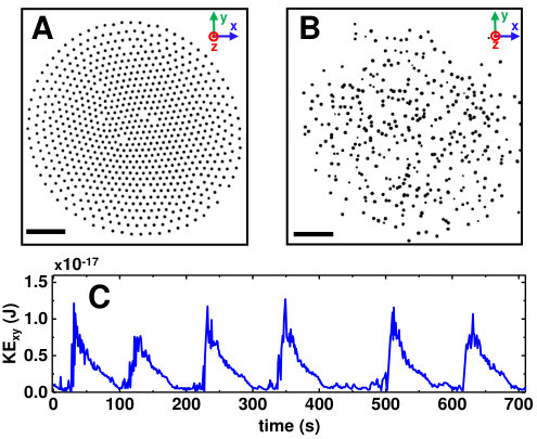 Figure 1
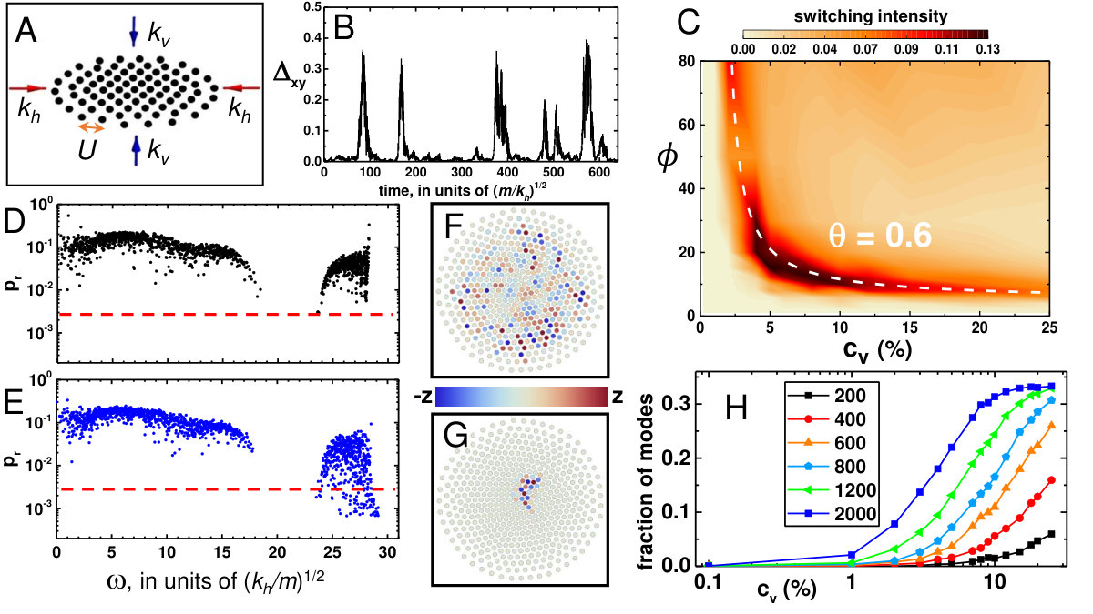 Figure 2
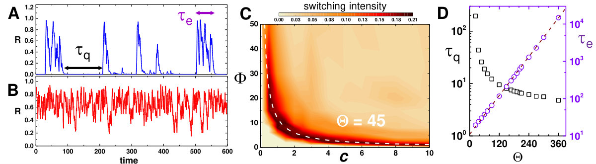 Figure 3
 Figure 4
Peer Reviews
No public reviews on file for this paper yet. If you reviewed it on a platform where reviews are public (OpenReview, ICLR, NeurIPS, ICML), you can paste yours below so the community can read it here.
Videos
No videos yet. Explain this paper in a talk, walkthrough, or lecture? Add one.
Taxonomy
TopicsTheoretical and Computational Physics · Stochastic processes and statistical mechanics · Advanced Thermodynamics and Statistical Mechanics
Intermittent “Turbulence” in a Many-body System
Guram Gogia
Wentao Yu
Justin C. Burton
Department of Physics, Emory University, Atlanta, GA, 30322
Abstract
In natural settings, intermittent dynamics are ubiquitous and often arise from a coupling between external driving and spatial heterogeneities. A well-known example is the generation of transient, turbulent “puffs” of fluid through a pipe with rough walls. Here we show how similar dynamics can emerge in a discrete, crystalline system of particles driven by noise. Polydispersity in particle masses leads to localized vibrational modes that effectuate a transition to a gas-like phase. A minimal model for the evolution of the system’s mechanical energies exhibits quasi-cyclic oscillations, and a single, dimensionless number captures the essential features of the intermittent dynamics, analogous to the Reynolds number for pipe flow.
The dynamics of complex systems that are driven away from equilibrium are usually characterized by minor fluctuations around some steady state, which are abruptly punctuated by a “big jump” Goldenfeld and Kadanoff (1999) leading to a dramatically different state. The climate oscillates between hot and cold regimes over millennia Petit et al. (1999), lakes switch between high- and low-nutrient regimes on decade-long time-scales van Nes et al. (2007), and rain showers pop up for a few minutes during summer afternoons. In spatially extended complex “ecologies”, such as vegetation D’Odorico et al. (2006) and power grids Nesti et al. (2018), spatio-temporal intermittency emerges due to coupling between external random forcing and the underlying structure.
A classical physical example of intermittent dynamics is transitional pipe flow Eckhardt et al. (2007), where laminar fluid flow develops spatially disordered and transient turbulent “puffs” for intermediate flow velocities. Since laminar flow in a pipe is linearly stable for all Reynolds numbers (Re) Lessen et al. (1968), the emergence of turbulence requires a finite disturbance, such as rough walls Nikuradze (1933) or other localized perturbations Reynolds (1883); Hof et al. (2003). Despite tremendous progress in experiment Avila et al. (2011) and theory Chaté and Manneville (1987); Barkley (2016); Shih et al. (2016); Manneville (2016) to capture the statistical properties of turbulence, the exact mechanism of cooperation between structural perturbations and the fluid flow remains elusive. The main challenge, as in other complex systems, lies in relating the local spatiotemporal interactions to the system-wide intermittent behavior.
Here we illustrate this connection in a simple, many-body system that manifests intermittent “turbulence”. A spatially-extended, horizontal layer of charged particles, forced vertically by white noise, continuously switches between crystalline and gas-like (turbulent) states. Particle polydispersity leads to spatially-localized vibrational modes that are necessary for the switching to occur. Upon excitation, these modes nonlinearly couple to other modes and redistribute the energy. Furthermore, we introduce a minimal model for the evolution of the total mechanical energy in the vertical and horizontal directions, reminiscent of stochastic predator-prey systems used to describe turbulence Shih et al. (2016). In both the simulation and the model, a single dimensionless number that incorporates external driving, dissipation, and disorder, successfully predicts the intermittent dynamical regime.
Experiments — The work described here was primarily motivated by recent experimental observations of emergent, intermittent dynamics in a quasi-2D dusty plasma crystal Gogia and Burton (2017). In the experiment, hundreds of electrostatically-levitated microspheres switch between crystalline (Fig. 1A) and gas-like states (Fig. 1B). Fig. 1C shows the average kinetic energy per particle in the imaging plane. The system is inherently nonequilibrium; energy is sourced from the plasma environment, leading to large-amplitude oscillations of each particle in Nunomura et al. (1999); Samarian et al. (2001); Marmolino (2011); Harper et al. (2019). Accompanying numerical simulations indicated that switching could only emerge if the particles have some finite size variation. This quenched disorder lead to localized melting which rapidly spread throughout the crystal. Here we generalize these results and identify the key ingredients for this class of intermittent, “turbulent” dynamics in a many-body system.
Numerical Simulations — We used a custom molecular dynamics code to simulate particles that interact via a finite-ranged pair potential, , where is the characteristic energy scale, is the particle separation, and is the screening length. The particles are spatially confined vertically and horizontally through harmonic potentials, and , where and are the respective spring constants (Fig. 2A). Particles were initially placed at random locations in the -plane and then quenched to the nearest local potential energy minimum using the FIRE algorithm Bitzek et al. (2006). The anisotropic confinement () leads to a separation of normal mode frequencies associated with in-plane and out-of-plane motion. In addition, we introduce two non-conservative forces: a hydrodynamic drag force, , where is the dissipation rate, and a spatially-uniform Langevin force in the -direction to stimulate vertical oscillations, , where is a Wiener process with zero mean and unit standard deviation, is the power delivered by the noise, and is the simulation time step. The particle positions and velocities were advanced in time using velocity-Verlet integration.
For identical particles, the noisy forcing only produced vertical motion in the system’s center-of-mass. To realize intermittent dynamics, we introduced quenched disorder by choosing the particle masses from a Gaussian distribution with mean and coefficient of variation . With these parameters, we identify a characteristic mass (), length (), and time () scale in the system. In what follows, all variables have been scaled by these units. The intermittent dynamics manifest as punctuated cascades of energy from the vertical to the horizontal directions, as illustrated by the fractional horizontal kinetic energy, , shown in Fig. 2B. Crystalline states correspond to , and gas-like states correspond to , where the upper limit corresponds to energy equipartition among the degrees of freedom. However, intermittent dynamics were only observed for a small range of parameters. To illustrate this, we characterized the switching intensity in the dynamics by integrating the Fourier transform of over frequencies smaller than 0.02 Hz, which corresponds to intermittency periods longer than 50 s (Fig. S3 sup ). A heatmap of the switching intensity (Fig. 2C) indicates a distinct regime of intermittent dynamics characterized by an inverse relationship between and . Too much disorder or stochastic forcing leads to a perpetual gas-like state, and too little leads to a stable crystalline state.
The transition to the gas-like state is rather abrupt since a copious amount of excess energy can be stored in the vertical oscillations (Suppl. Movie sup ). An analysis of the harmonic vibrational modes in the system illustrates how quenched disorder facilitates this transition Henkes et al. (2012); Bottinelli and Silverberg (2017); Burton and Nagel (2016). For each system, the Hessian matrix was computed about the local potential energy minimum corresponding to the crystalline state (sup ). The 3 eigenvalues of this matrix correspond to squares of mode frequencies, whereas the normalized eigenvectors are the polarizations of the particle displacements. The localization of each mode was characterized using the participation ratio Burton and Nagel (2016); sup . Modes with represent the collective motion of many particles, whereas the modes with correspond to localized modes consisting of a few particles.
Figure 2D-E shows versus angular frequency for a monodisperse (D) and a polydisperse (E) system comprised of = 500 particles. There are two distinct frequency bands. High frequency modes ( 25) correspond to vertical motion, and low frequency modes ( 20) correspond to horizontal motion. A frequency gap separates these bands and suppresses mode coupling. A typical extended vertical mode is shown in Fig. 2F. A small amount of quenched disorder in particle mass leads to localized modes (Fig. 2G) with in the vertical frequency band, yet leaves the horizontal frequency band essentially unchanged. Upon excitation with a spatially-uniform (wavevector ) stochastic force, these low- modes are preferentially excited since they contain low- Fourier components. These modes are also more susceptible to nonlinear coupling since the relative amplitude of motion between neighboring particles is larger. Consequently, they serve as the progenitors of the energy cascade from vertical to horizontal motion.
Furthermore, we quantified the fraction of vibrational modes with below the lowest value for a monodisperse sample (), as shown by the dashed red lines in Fig. 2D-E. This fraction increased monotonically with the amount of disorder and the ratio of vertical to horizontal confinement, . As illustrated in Fig. 2H, for strong confinement, the gap between the frequency bands is large and a small amount of disorder can quickly lead to mode localization. For weak confinement, the gap is small or nonexistent and mode localization requires more structural disorder. For all the data shown in Fig. 2H, intermittent switching occurs when the fraction of low- modes is approximately 0.07–0.2. In this manner, the linear, equilibrium properties can inform system’s nonequilibrium dynamical response Mukamel (2000).
In order to better characterize the dynamical behavior, we identified 5 relevant dimensionless numbers through Buckingham’s Pi theorem: , , , , and . characterizes the degree of structural disorder. and determine the degree of quasi-2D confinement. If either number is too small, then the system’s equilibrium configuration will be “buckled” into the -direction (Fig. S2 sup ). determines the quality factor of underdamped vertical oscillations. Lastly, , is the only number associated with the external forcing. This can be intuited as the amount of noisy power necessary for a stochastic, damped harmonic oscillator to reach an average amplitude , (Fig. S6) sup . This amplitude threshold will induce rearrangements in the crystalline lattice since the particle spacing is also of order , similar to the Lindemann criteria in classical melting Lindemann (1910). For a thermal, Brownian oscillator, would assume the role of in our simulations.
We can form a single dimensionless number that describes the system-wide, intermittent dynamics by considering the role of disorder on the vertical oscillations. Since each particle has a slightly different mass, their vertical frequencies vary, , where . For to be significant, it must be larger than , which determines the broadness of their response in frequency space. If is too large, the oscillators will be strongly coupled. Thus, by multiplying the stochastic forcing, , by the disorder in frequency space, , we obtain
[TABLE]
characterizes the ratio of energy input to dissipation, modulated by disorder. This is analogous to a “friction factor” in transitional pipe flow that includes the cooperative effects of wall roughness and Reynolds number Goldenfeld (2006). For reasonable values of the other dimensionless numbers, intermittent dynamics should occur along contours of constant , as shown by the white dashed line in Fig. 2C (Fig. S5 sup ).
Minimal Model for Many-Body Turbulence — An ecosystem of two or more competing species is an archetypal model for studying oscillations in dynamical systems Lotka (1910); Volterra (1926). In addition to intermittent turbulence in pipe flow Shih et al. (2016), other recent examples include the oscillation of the light emission from dust-forming plasmas Ross and McKenzie (2016), and intermittent precipitation in climate models Koren and Feingold (2011). In our many-body system, we can derive a two-species framework by considering the total horizontal mechanical energy () as a predator, and the total vertical mechanical energy () as a prey to be consumed:
[TABLE]
Here we have assumed that kinetic and potential energies are equipartitioned in each direction, so that and . The first terms on the right hand side in 2 and 3 correspond to the power dissipated through hydrodynamic damping, , where the sum runs over each particle. The second term, derived from classical scattering theory sup , characterizes “predation” and obeys energy conservation. The constant controls the coupling between vertical and horizontal energies, and parameterizes the polydispersity in the many-body system. Finally, the third term in Eq. 3 represents the instantaneous power delivered in the vertical direction, , where and is the average power. Similar noise terms are commonly used to model demographic stochasticity in ecological systems, often resulting in population oscillations McKane and Newman (2005).
These equations recreate the three observed dynamical regimes. To directly compare with the numerical simulations, we define as the fractional horizontal mechanical energy, in analogy with (Fig. 2B). For intermediate values of and , exhibits intermittent behavior (Fig. 3A), whereas sufficiently increasing either parameter results in a perpetually excited, equipartitioned state () (Fig. 3B). The dependence of the switching intensity on both parameters can be seen in Fig. 3C. The heatmap shows that there is a distinct region where intermittent dynamics can be observed. In a similar manner to the particle-based simulations, this regime can be described by a single dimensionless number, , which represents the ratio of the energy input and coupling to dissipation. Intermittent dynamics are only observed for (Fig. 3C and Fig. S8 sup ), in analogy to transitional pipe flow, where intermittent turbulence is observed for intermediate Reynolds numbers ( Re ) Kerswell (2005).
Furthermore, transitional pipe flow is known to exhibit spatiotemporal, critical behavior Goldenfeld and Shih (2017). The lifetime statistics and universality class are related to directed percolation where laminar flow acts as a nonequilibrium absorbing state Shih et al. (2016); Goldenfeld and Shih (2017); Pomeau (1986, 2016); Barkley (2016). For intermittent turbulence with spatially-separated, coexisting, independent “puffs”, the lifetime of the turbulent state scales super-exponentially with Reynolds number Avila et al. (2011); Shih et al. (2016). For a given in our minimal model, the probability distribution of both excited () and quiescent () state lifetimes have exponential tails (Fig. S9 sup ), and the mean lifetime of the excited state scales exponentially with (Fig. 3D). This scaling originates from the memoryless noise driving the system. If our many-body system were spatially-extended and could support multiple excited, gas-like regions, we would expect extreme value statistics and subsequently, super-exponential behavior Goldenfeld and Shih (2017).
Summary — Intermittent dynamics are commonly observed in natural systems but rarely understood. Here we presented a distinct mechanism to promote intermittent dynamics in a tractable, many-body system. A layer of polydisperse, interacting particles, damped by the environment and driven anisotropically by noise, can intermittently transition between gaseous and crystalline states. Spatial heterogeneities, in the form of localized vibrational modes, couple with the external noise to facilitate this transition. In this sense external noise acts as an engine that drives the system in one direction, and structural heterogeneities act as a rudder that intermittently steers energy into other degrees of freedom. We also derived a single dimensionless number that characterizes the intermittent regime, in analogy to the Reynolds number in transitional pipe flow. Moreover, we provided a minimal model that captures the essential features of the many-body dynamics, and demonstrates a exponential scaling of the lifetimes of the excited states, a feature only recently confirmed for the lifetime of turbulent “puffs” in fluid flow. We hope these results lead to further connections between simple, discrete particle dynamics and natural complex systems.
Acknowledgements — We acknowledge financial support from the National Science Foundation Grant No. 1455086. We gratefully acknowledge H.-Y. Shih and N. Goldenfeld for stimulating discussions about predator-prey systems. We would like to thank J. Mendez, M. Kawamura, H. Saul, J. Silverberg, A. Roman, I. Nemenman, M. Martini, B. Beal, and B. Doolittle for useful discussions.
The reference list from the paper itself. Each links out to its DOI / PubMed record.
- 1Goldenfeld and Kadanoff (1999) N. Goldenfeld and L. P. Kadanoff, Science 284 , 87 (1999).
- 2Petit et al. (1999) J.-R. Petit, J. Jouzel, D. Raynaud, N. I. Barkov, J.-M. Barnola, I. Basile, M. Bender, J. Chappellaz, M. Davis, G. Delaygue, and et al., Nature 399 , 429 (1999).
- 3van Nes et al. (2007) E. H. van Nes, W. J. Rip, and M. Scheffer, Ecosystems 10 , 17 (2007).
- 4D’Odorico et al. (2006) P. D’Odorico, F. Laio, and L. Ridolfi, Geophys. Res. Lett. 33 , L 19404 (2006).
- 5Nesti et al. (2018) T. Nesti, A. Zocca, and B. Zwart, Phys. Rev. Lett. 120 , 258301 (2018).
- 6Eckhardt et al. (2007) B. Eckhardt, T. M. Schneider, B. Hof, and J. Westerweel, Annu. Rev. Fluid Mech. 39 , 447 (2007).
- 7Lessen et al. (1968) M. Lessen, S. G. Sadler, and T.-Y. Liu, The Physics of Fluids 11 , 1404 (1968).
- 8Nikuradze (1933) J. Nikuradze, v DI Forschungsheft 361 (1933).