NADA-FLD: A General Relativistic, Multi-dimensional Neutrino-hydrodynamics Code Employing Flux-limited Diffusion
Ninoy Rahman (1,2), Oliver Just (3), and H.-Thomas Janka (1) ((1) MPI, f. Astrophysics, Garching, (2) Physik Department, TUM, (3) ABBL, RIKEN)

TL;DR
The paper introduces NADA-FLD, a new multi-dimensional neutrino-hydrodynamics code in general relativity using flux-limited diffusion, tested on supernova models and showing good agreement with existing codes.
Contribution
NADA-FLD is a novel code that combines GR, multi-dimensional neutrino transport, and flux-limited diffusion with explicit schemes for lateral diffusion and advection.
Findings
Good agreement with ALCAR code in Newtonian models
Reproduces main effects of GR in supernova simulations
Demonstrates stability and accuracy in toy-model tests
Abstract
We present the new code NADA-FLD to solve multi-dimensional neutrino-hydrodynamics in full general relativity (GR) in spherical polar coordinates. The energy-dependent neutrino transport assumes the flux-limited diffusion (FLD) approximation and evolves the neutrino energy densities measured in the frame comoving with the fluid. Operator splitting is used to avoid multi-dimensional coupling of grid cells in implicit integration steps involving matrix inversions. Terms describing lateral diffusion and advection are integrated explicitly using the Allen-Cheng or the Runge-Kutta-Legendre method, which remain stable even in the optically thin regime. We discuss several toy-model problems in one and two dimensions to test the basic functionality and individual components of the transport scheme. We also perform fully dynamic core-collapse supernova (CCSN) simulations in spherical symmetry.…
Click any figure to enlarge with its caption.
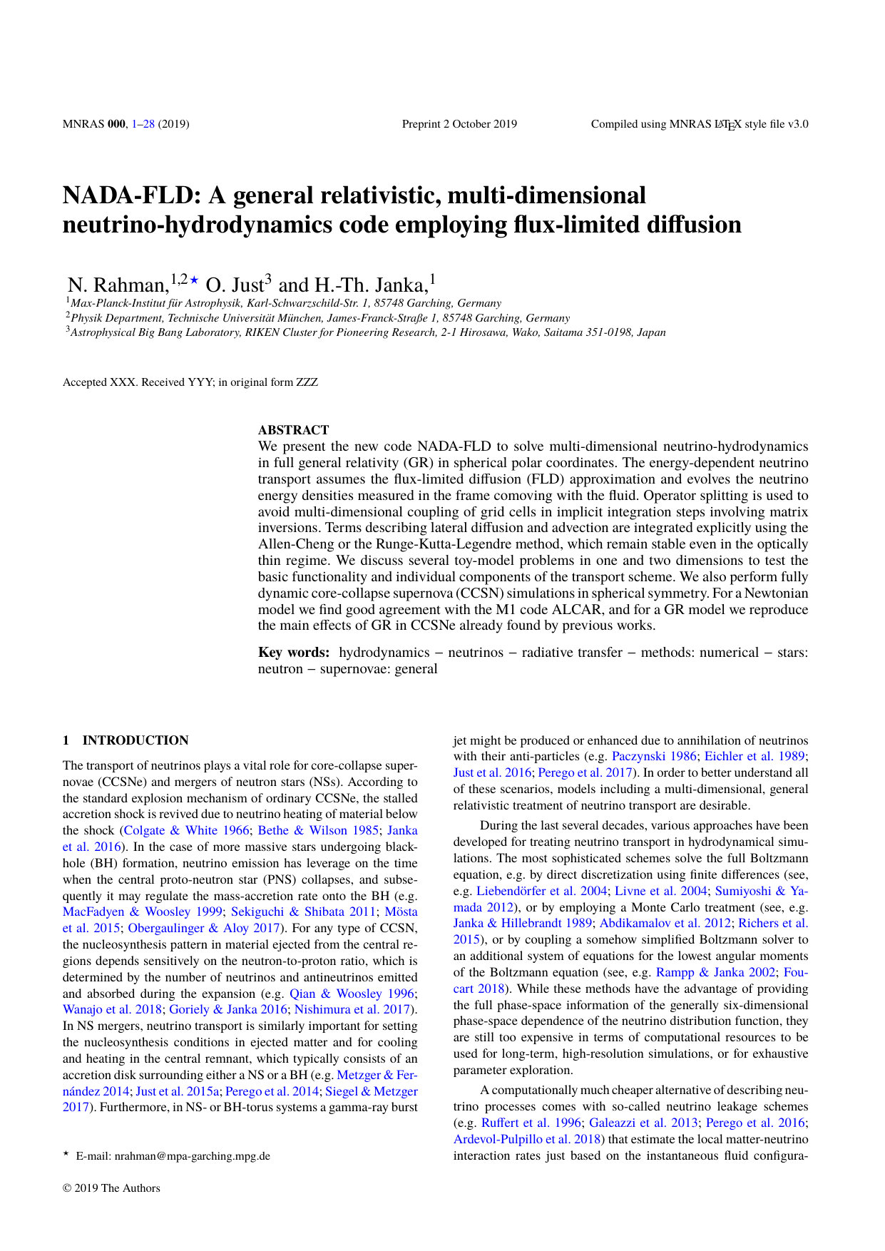 Figure 1
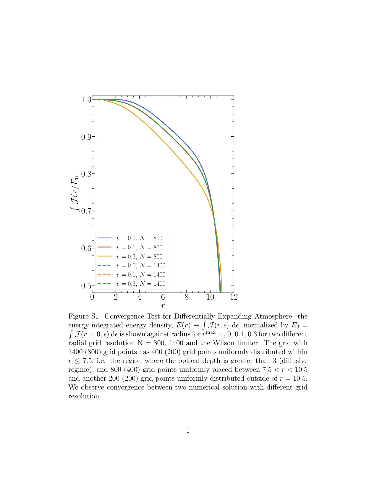 Figure 2
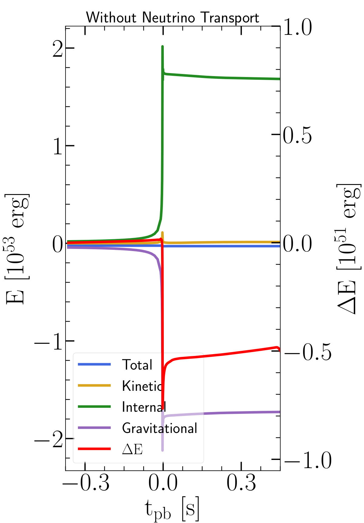 Figure 3
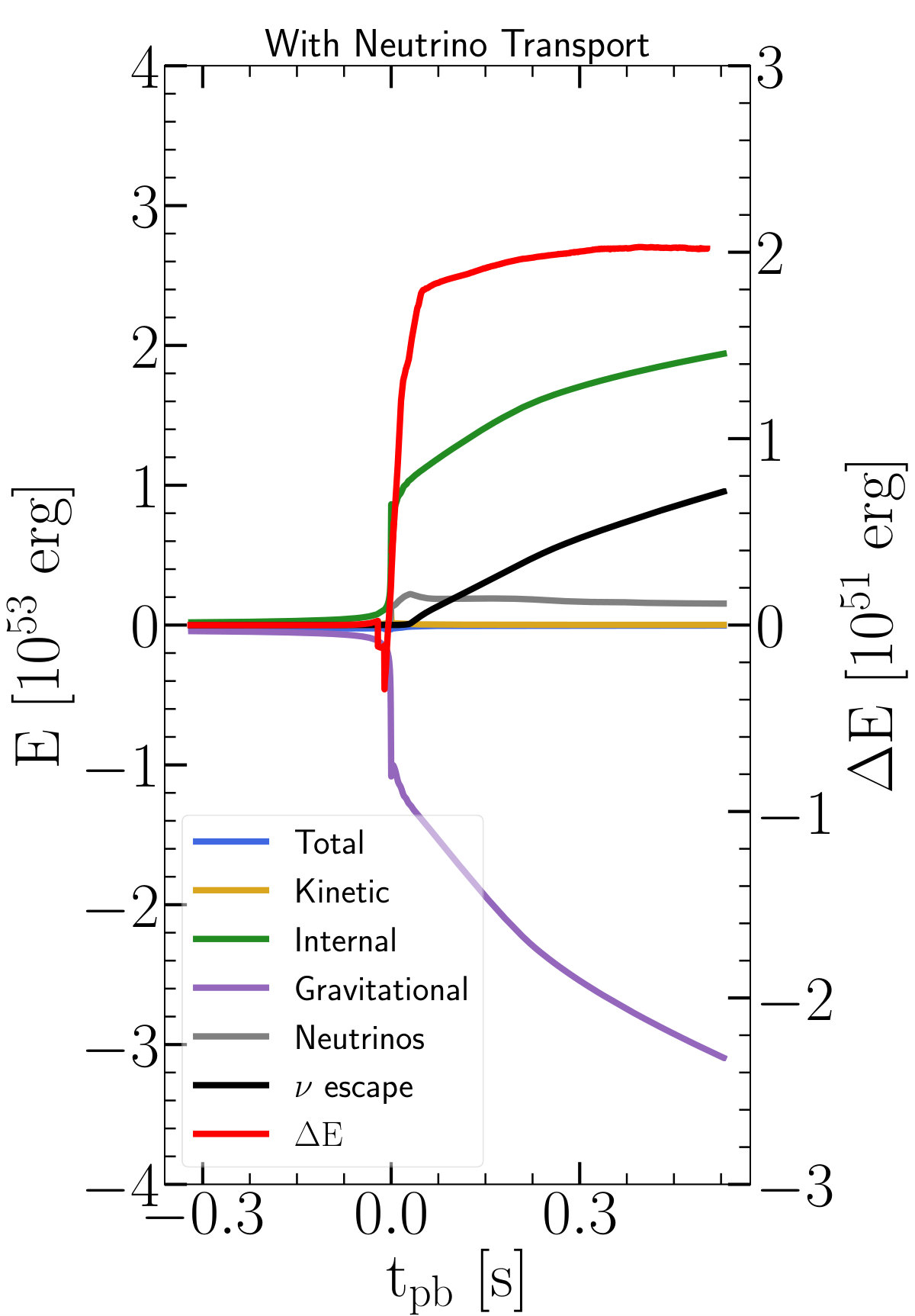 Figure 4
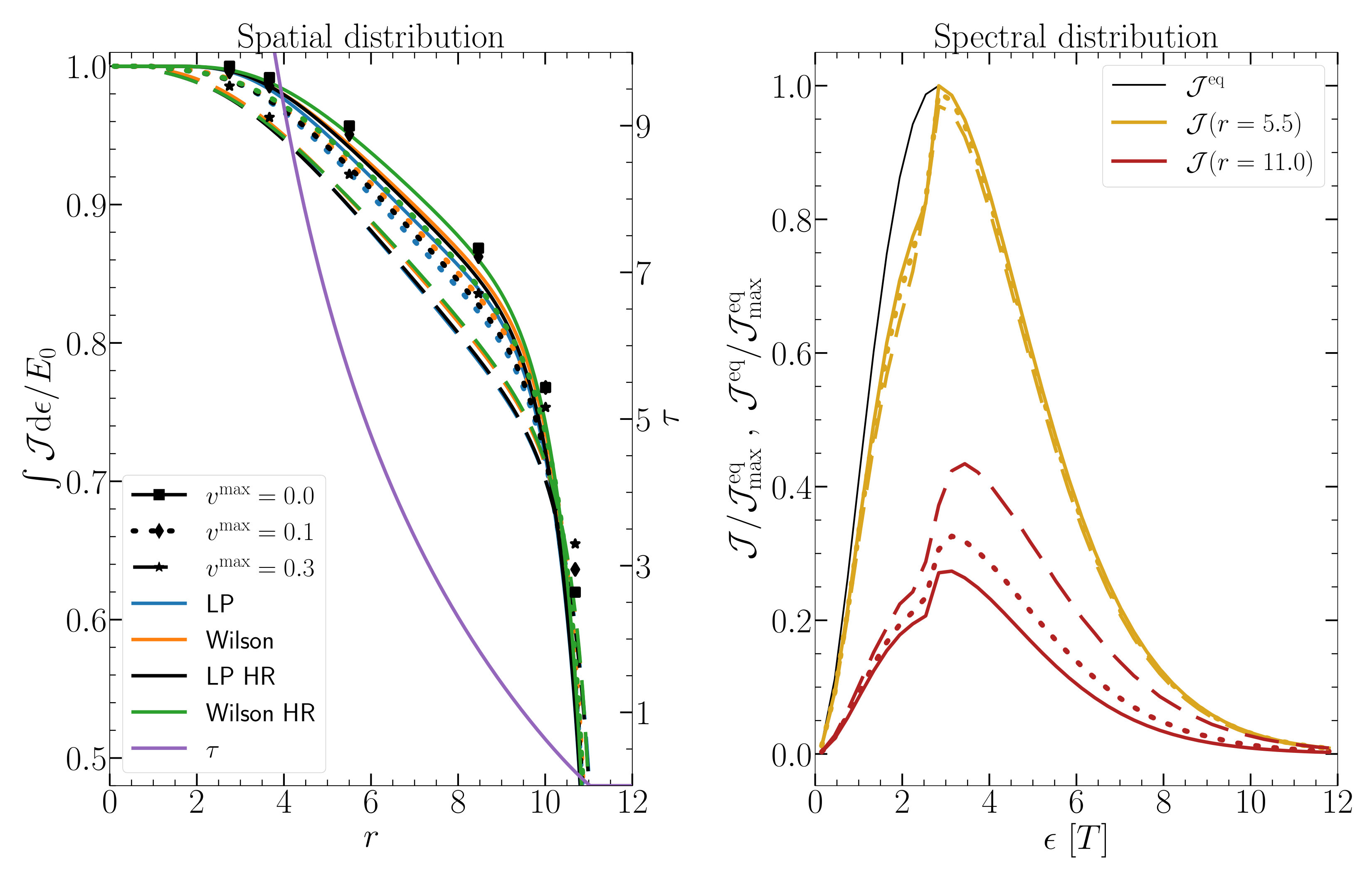 Figure 5
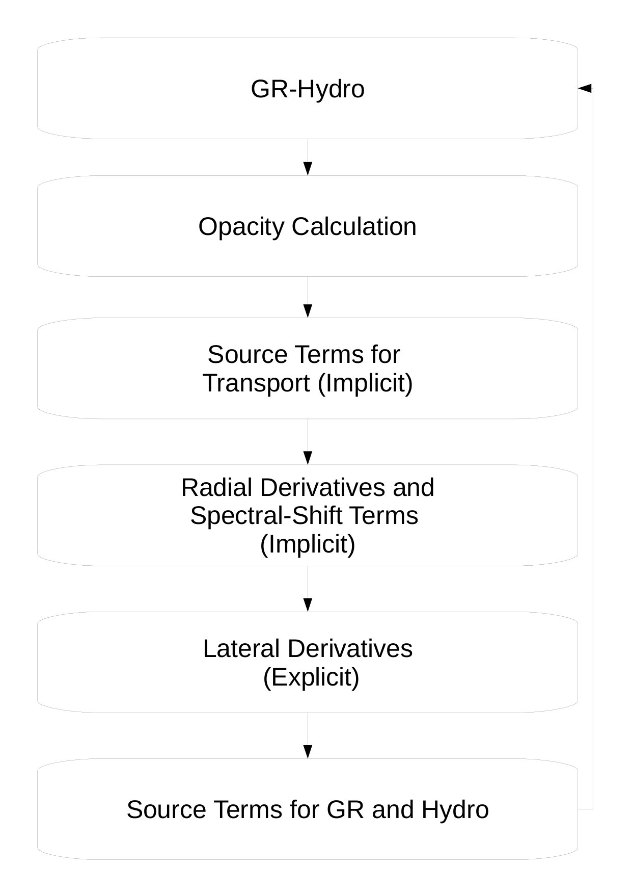 Figure 6
 Figure 7
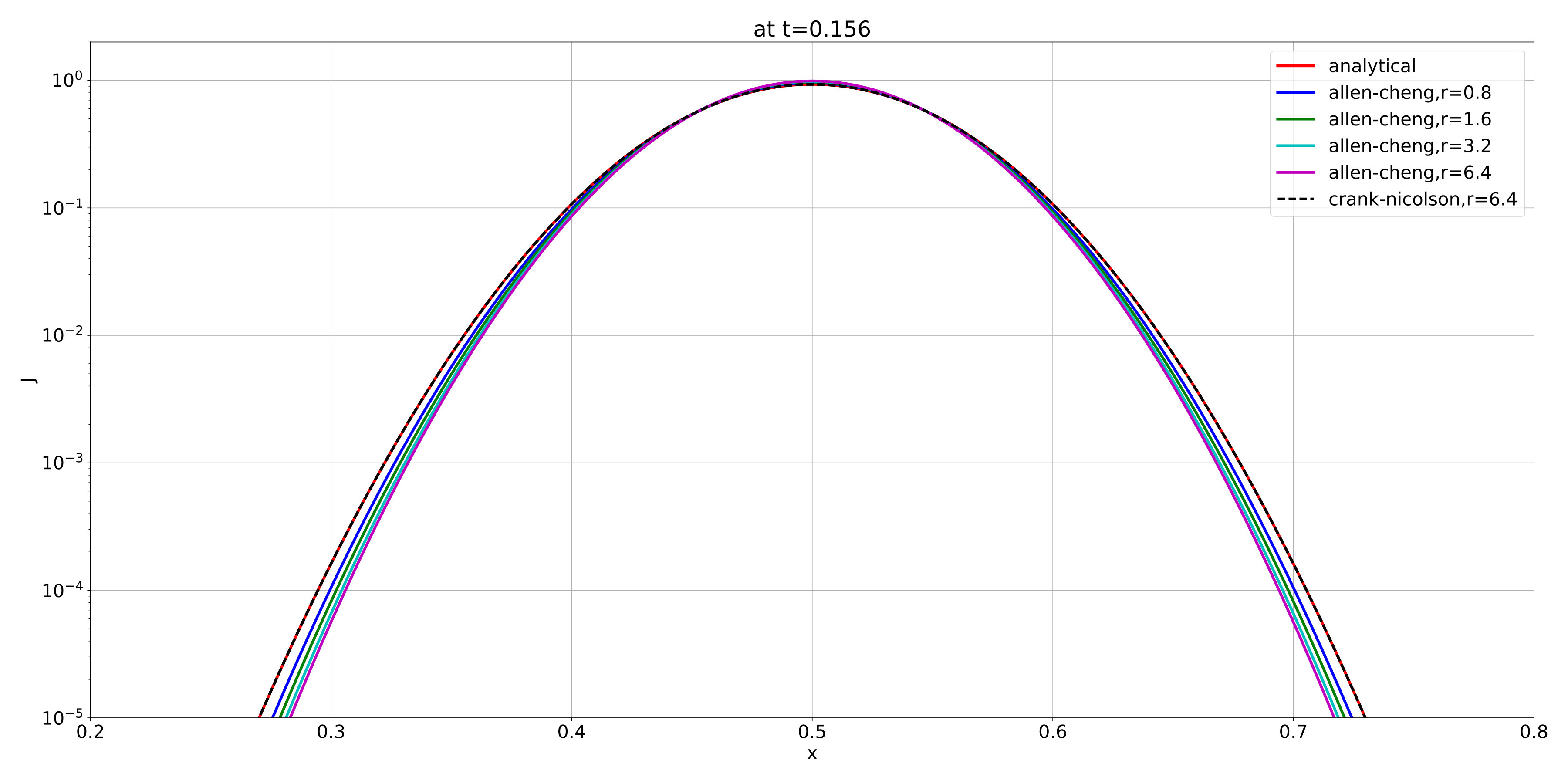 Figure 8
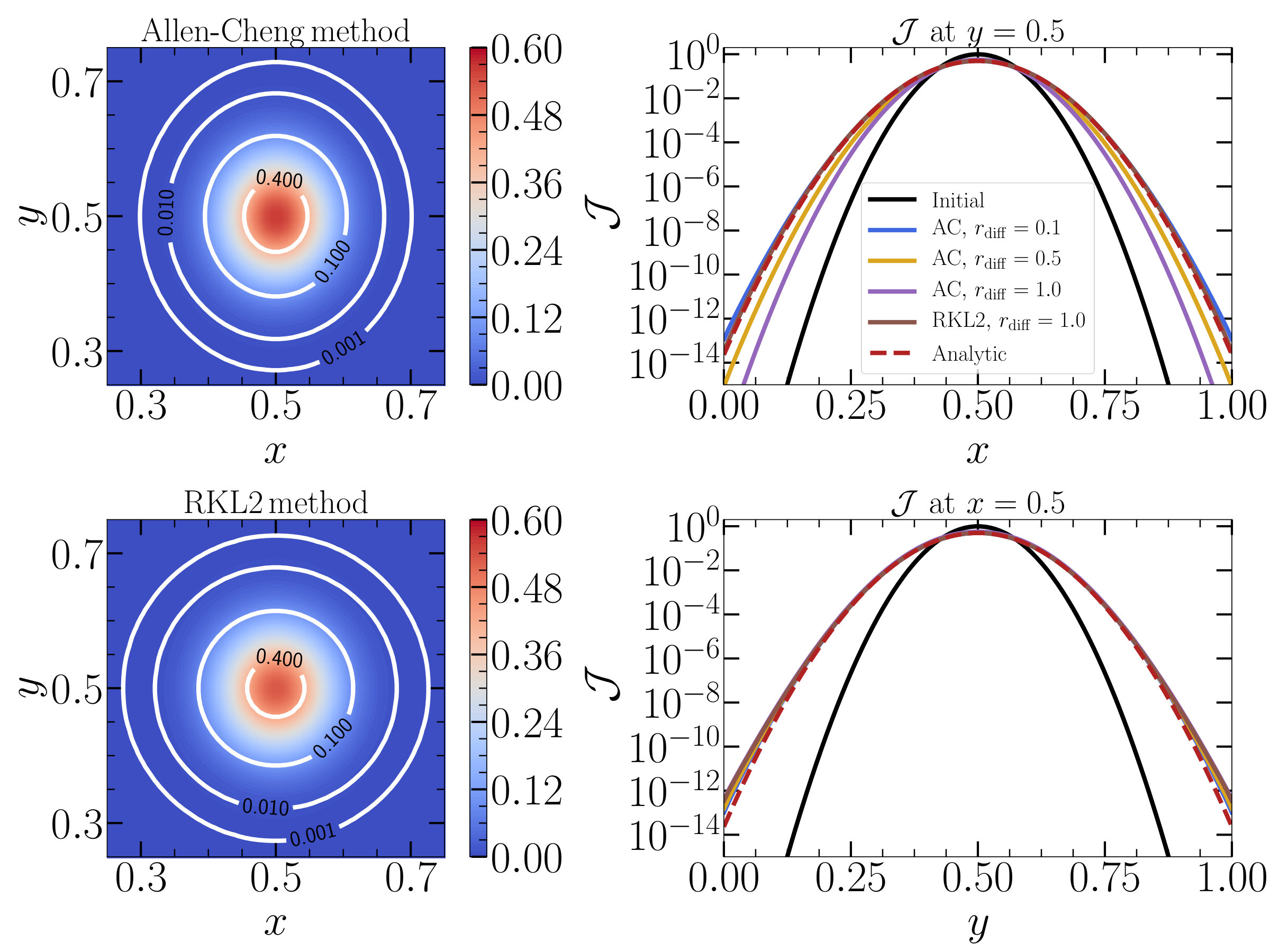 Figure 9
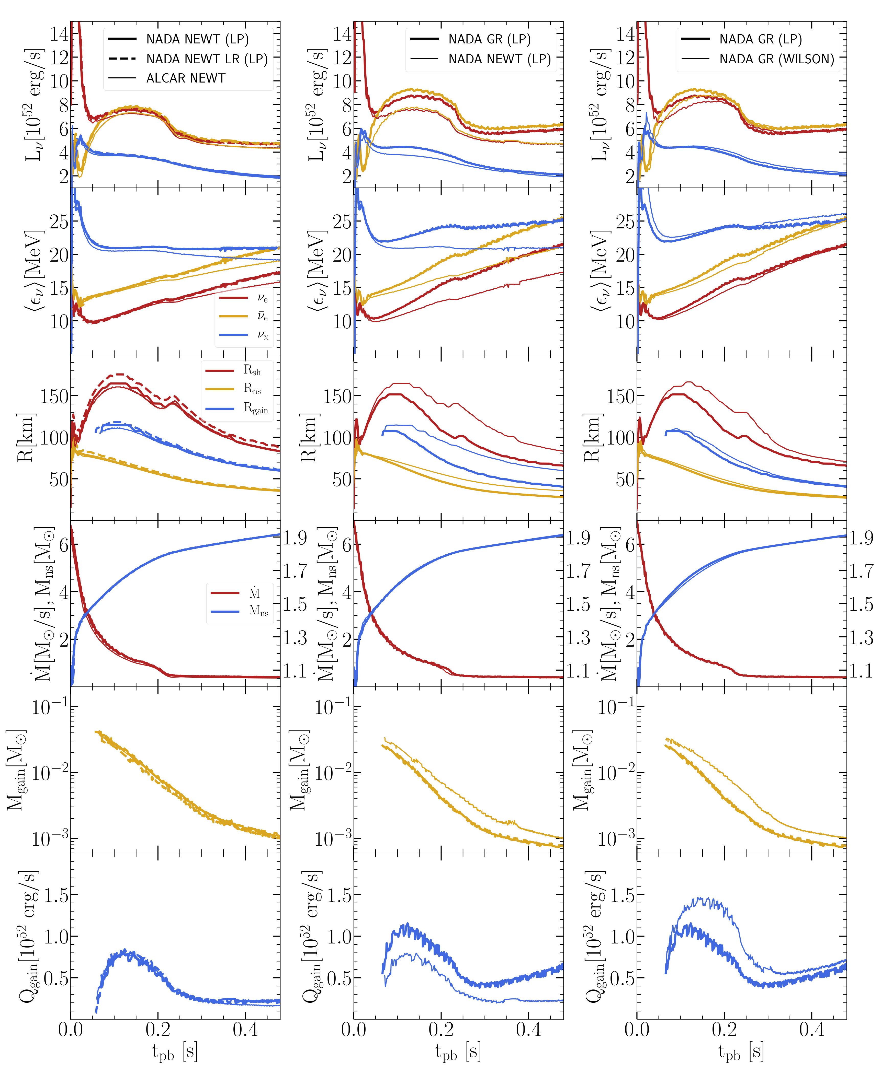 Figure 10
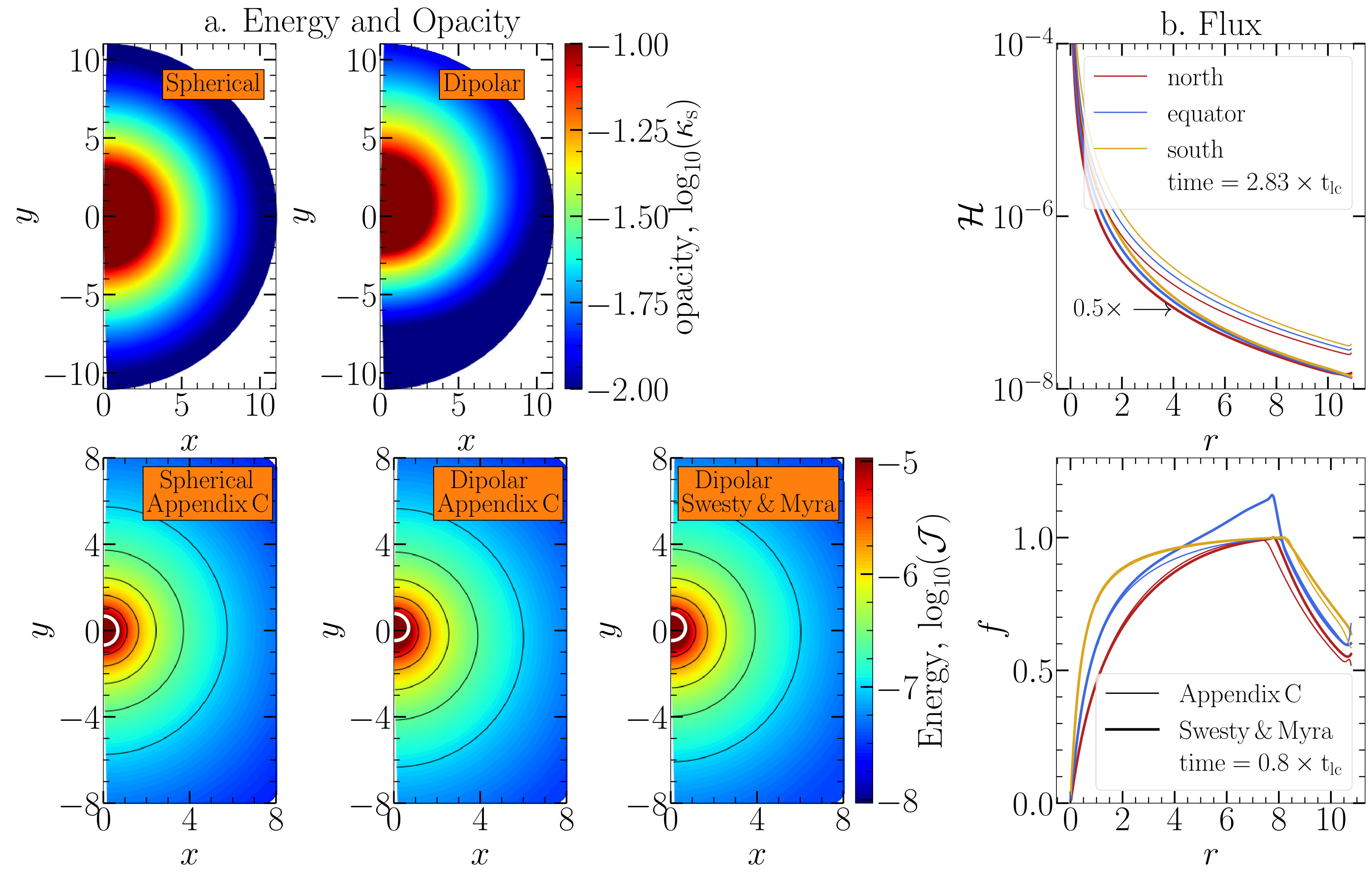 Figure 11
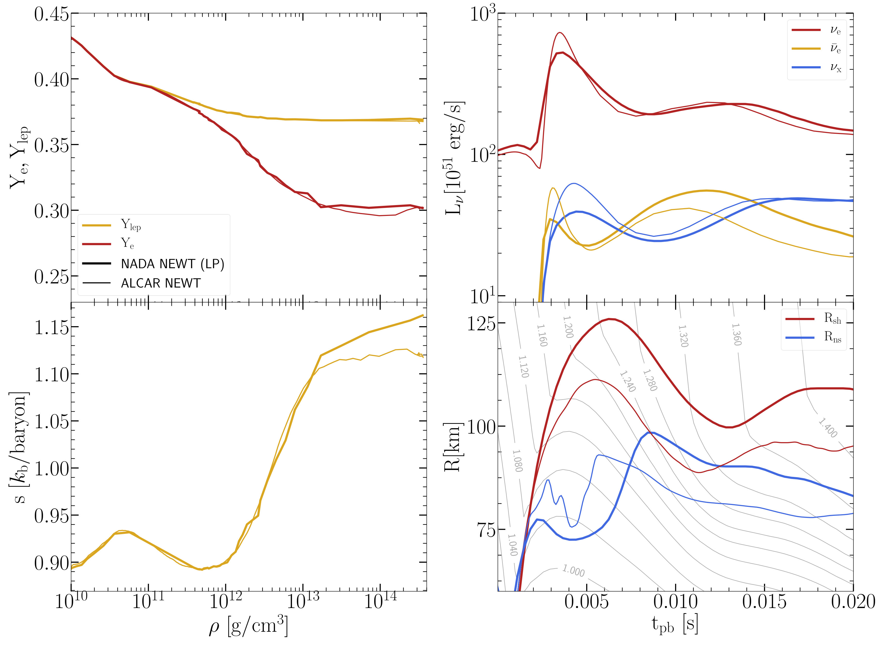 Figure 12
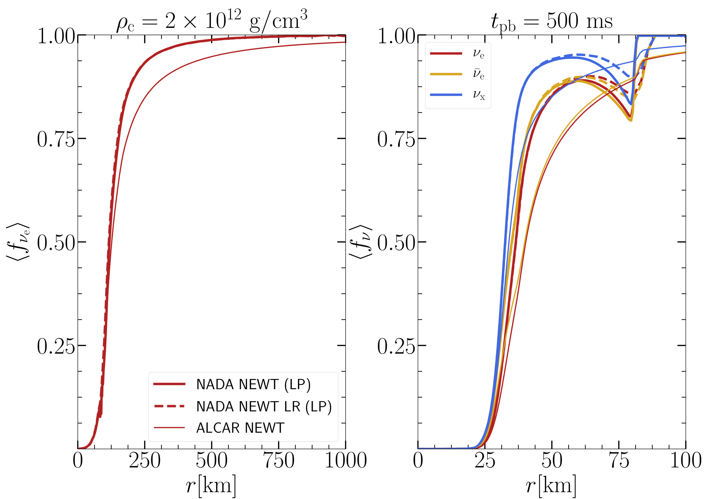 Figure 13
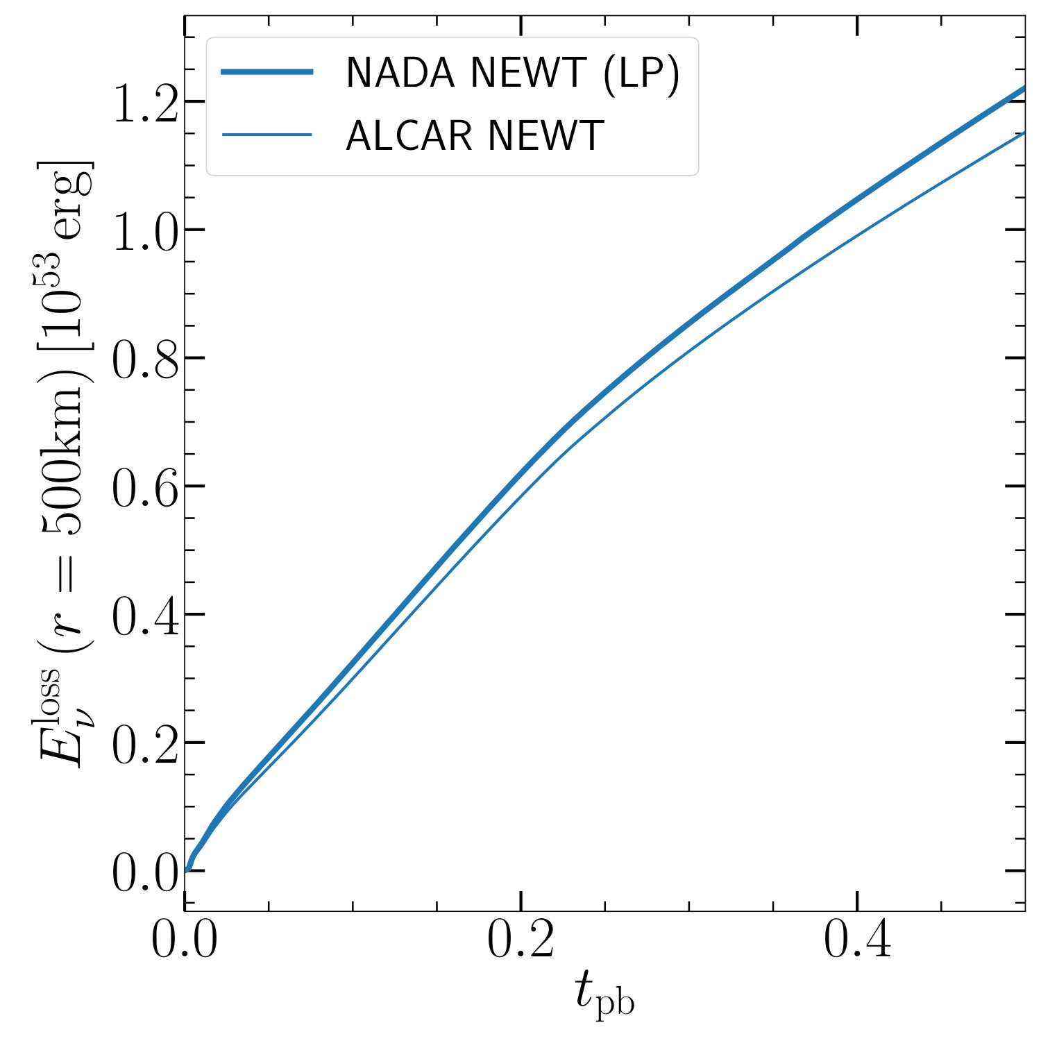 Figure 14
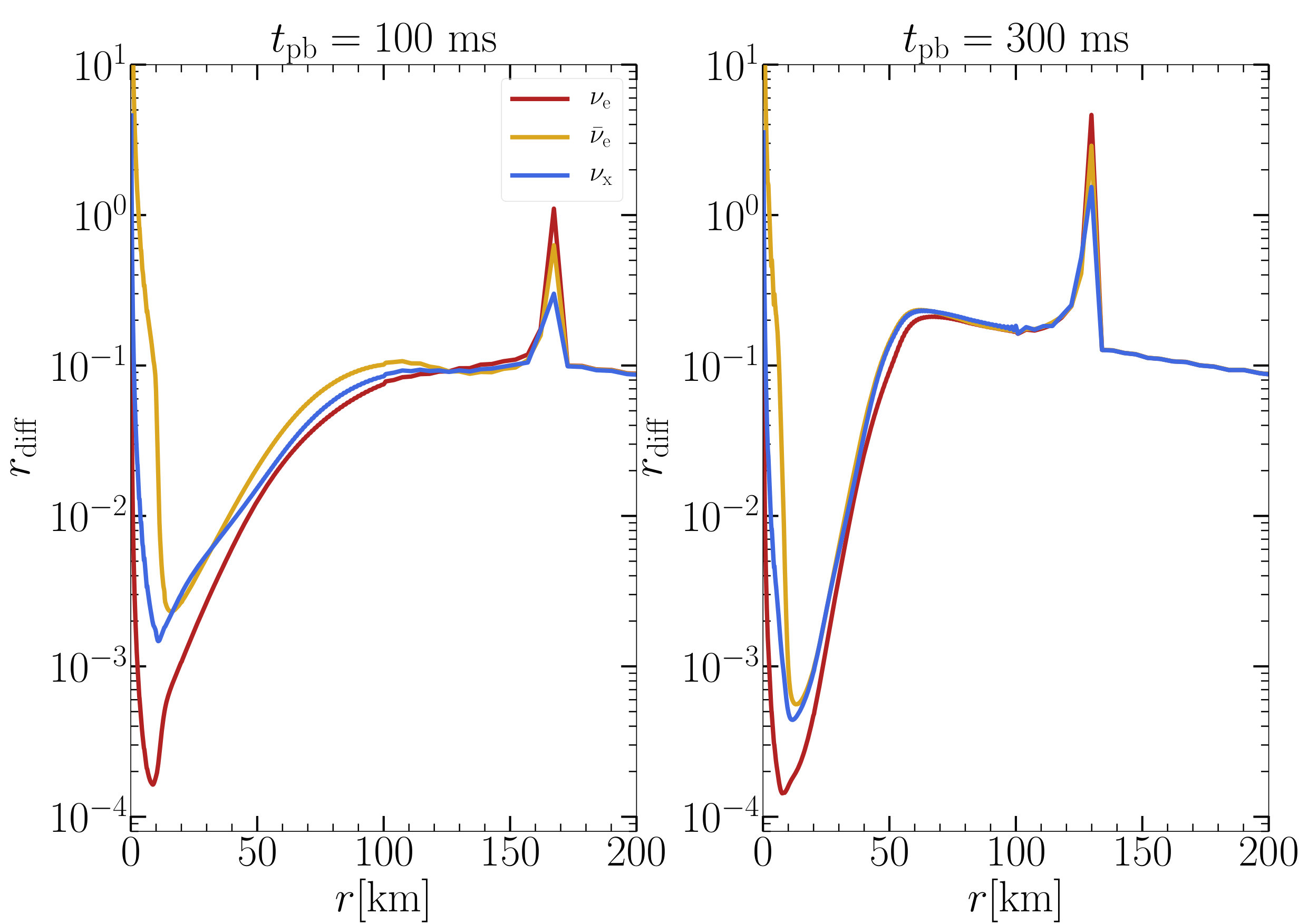 Figure 15
| CFL | resolution, | L2 error | error ratio |
|---|---|---|---|
| 1.0 | 128 | 0.258 | |
| 256 | 0.054 | 4.751 | |
| 512 | 0.013 | 4.023 | |
| 10.0 | 128 | 0.259 | |
| 256 | 0.055 | 4.711 | |
| 512 | 0.013 | 4.062 |
| resolution, | L2 error | error ratio | |
|---|---|---|---|
| 3.2 | 200 | 0.0885 | |
| 1.6 | 200 | 0.0583 | 1.518 |
| 0.8 | 200 | 0.0359 | 1.623 |
| 0.4 | 200 | 0.0206 | 1.742 |
| 0.2 | 200 | 0.0089 | 2.314 |
| 0.1 | 200 | 0.0037 | 2.405 |
| Reaction | Neutrino |
|---|---|
| 0th angular moment of distribution function in comoving frame | eq. (19) | |
| 1st angular moment of distribution function in comoving frame | eq. (19) | |
| 2nd angular moment of distribution function in comoving frame | eq. (19) | |
| 0th angular moment of distribution function in lab frame | eq. (22) | |
| 1st angular moment of distribution function in lab frame | eq. (22) | |
| 2nd angular moment of distribution function in lab frame | eq. (22) | |
| 0th projection of in lab frame | eq. (125) of Cardall et al. (2013) | |
| 1st projection of in lab frame | eq. (126) of Cardall et al. (2013) | |
| 2nd projection of in lab frame | eq. (127) of Cardall et al. (2013) | |
| 3rd projection of in lab frame | eq. (128) of Cardall et al. (2013) |
Peer Reviews
No public reviews on file for this paper yet. If you reviewed it on a platform where reviews are public (OpenReview, ICLR, NeurIPS, ICML), you can paste yours below so the community can read it here.
Videos
No videos yet. Explain this paper in a talk, walkthrough, or lecture? Add one.
NADA-FLD: A general relativistic, multi-dimensional neutrino-hydrodynamics code employing flux-limited diffusion
N. Rahman,1,2 O. Just3 and H.-Th. Janka,1
1Max-Planck-Institut für Astrophysik, Karl-Schwarzschild-Str. 1, 85748 Garching, Germany
2Physik Department, Technische Universität München, James-Franck-Straße 1, 85748 Garching, Germany
3Astrophysical Big Bang Laboratory, RIKEN Cluster for Pioneering Research, 2-1 Hirosawa, Wako, Saitama 351-0198, Japan E-mail: [email protected]
(Accepted XXX. Received YYY; in original form ZZZ)
Abstract
We present the new code NADA-FLD to solve multi-dimensional neutrino-hydrodynamics in full general relativity (GR) in spherical polar coordinates. The energy-dependent neutrino transport assumes the flux-limited diffusion (FLD) approximation and evolves the neutrino energy densities measured in the frame comoving with the fluid. Operator splitting is used to avoid multi-dimensional coupling of grid cells in implicit integration steps involving matrix inversions. Terms describing lateral diffusion and advection are integrated explicitly using the Allen-Cheng or the Runge-Kutta-Legendre method, which remain stable even in the optically thin regime. We discuss several toy-model problems in one and two dimensions to test the basic functionality and individual components of the transport scheme. We also perform fully dynamic core-collapse supernova (CCSN) simulations in spherical symmetry. For a Newtonian model we find good agreement with the M1 code ALCAR, and for a GR model we reproduce the main effects of GR in CCSNe already found by previous works.
keywords:
hydrodynamics neutrinos radiative transfer methods: numerical stars: neutron supernovae: general
††pubyear: 2019††pagerange: NADA-FLD: A general relativistic, multi-dimensional neutrino-hydrodynamics code employing flux-limited diffusion–C
1 Introduction
The transport of neutrinos plays a vital role for core-collapse supernovae (CCSNe) and mergers of neutron stars (NSs). According to the standard explosion mechanism of ordinary CCSNe, the stalled accretion shock is revived due to neutrino heating of material below the shock (Colgate & White, 1966; Bethe & Wilson, 1985; Janka et al., 2016). In the case of more massive stars undergoing black-hole (BH) formation, neutrino emission has leverage on the time when the central proto-neutron star (PNS) collapses, and subsequently it may regulate the mass-accretion rate onto the BH (e.g. MacFadyen & Woosley 1999; Sekiguchi & Shibata 2011; Mösta et al. 2015; Obergaulinger & Aloy 2017). For any type of CCSN, the nucleosynthesis pattern in material ejected from the central regions depends sensitively on the neutron-to-proton ratio, which is determined by the number of neutrinos and antineutrinos emitted and absorbed during the expansion (e.g. Qian & Woosley 1996; Wanajo et al. 2018; Goriely & Janka 2016; Nishimura et al. 2017). In NS mergers, neutrino transport is similarly important for setting the nucleosynthesis conditions in ejected matter and for cooling and heating in the central remnant, which typically consists of an accretion disk surrounding either a NS or a BH (e.g. Metzger & Fernández 2014; Just et al. 2015a; Perego et al. 2014; Siegel & Metzger 2017). Furthermore, in NS- or BH-torus systems a gamma-ray burst jet might be produced or enhanced due to annihilation of neutrinos with their anti-particles (e.g. Paczynski 1986; Eichler et al. 1989; Just et al. 2016; Perego et al. 2017). In order to better understand all of these scenarios, models including a multi-dimensional, general relativistic treatment of neutrino transport are desirable.
During the last several decades, various approaches have been developed for treating neutrino transport in hydrodynamical simulations. The most sophisticated schemes solve the full Boltzmann equation, e.g. by direct discretization using finite differences (see, e.g. Liebendörfer et al. 2004; Livne et al. 2004; Sumiyoshi & Yamada 2012), or by employing a Monte Carlo treatment (see, e.g. Janka & Hillebrandt 1989; Abdikamalov et al. 2012; Richers et al. 2015), or by coupling a somehow simplified Boltzmann solver to an additional system of equations for the lowest angular moments of the Boltzmann equation (see, e.g. Rampp & Janka 2002; Foucart 2018). While these methods have the advantage of providing the full phase-space information of the generally six-dimensional phase-space dependence of the neutrino distribution function, they are still too expensive in terms of computational resources to be used for long-term, high-resolution simulations, or for exhaustive parameter exploration.
A computationally much cheaper alternative of describing neutrino processes comes with so-called neutrino leakage schemes (e.g. Ruffert et al. 1996; Galeazzi et al. 2013; Perego et al. 2016; Ardevol-Pulpillo et al. 2018) that estimate the local matter-neutrino interaction rates just based on the instantaneous fluid configuration without evolving (or evolving only in regions where neutrinos are trapped) conservation equations for neutrino energy and number. Moreover, several additional schemes have been designed for specific application purposes, including light-bulb schemes (e.g. Janka & Müller 1996), the fast-multigroup transport scheme (FMT; Müller & Janka 2015), the M0 scheme (Radice et al., 2016), or the isotropic-diffusion-source approximation (IDSA; Liebendörfer et al. 2009).
In the class of local-closure moment schemes only the lowest angular moments of the distribution function are dynamically evolved, while all higher-order moments are provided by an approximate closure relation as function of the evolved moments. In flux-limited diffusion (FLD) schemes only the zeroth-order moment (i.e. the energy density) is evolved, while in two-moment (M1) schemes additionally the first-order moment (flux density) is integrated. In the recent years a number of M1 schemes have been developed (O’Connor, 2015; Just et al., 2015b; Foucart et al., 2015; Kuroda et al., 2016; Skinner et al., 2019; Sekiguchi et al., 2012).
The concept of FLD was first introduced by Pomraning (1981) and Levermore & Pomraning (1981) and since then has been used, apart from many applications in the context of photon transport, for neutrino transport in CCSNe and PNS cooling (Bowers & Wilson, 1982; Bruenn, 1985; Burrows & Lattimer, 1986; Myra et al., 1987; Baron et al., 1989; Cernohorsky, 1990; Burrows et al., 2007; Lentz et al., 2015; Bruenn et al., 2018). Cooperstein & Baron (1992) derived the FLD equation correct to order . The maximum entropy principle was applied by Cernohorsky et al. (1989) in FLD to determine Eddington factors. Baron et al. (1989) generalized the FLD approach to the general relativistic context. An improved flux-limiter was suggested by Janka (1992) based on the comparison with a Monte-Carlo study. A two dimensional, multi-group (i.e. energy-dependent) FLD scheme for neutrinos was developed by Swesty & Myra (2009).
General relativistic (GR) radiative transfer as a scientific discipline was established with the formulation of the Boltzmann equation in GR by Lindquist (1966) and of the corresponding two moment formalism in Thorne (1981). Until rather recently, most numerical applications were restricted to spherical symmetry (e.g. Baron et al., 1989; Bruenn et al., 2001; Liebendörfer et al., 2004). A few years ago, multi-group GR transport has found its way into multiple dimensions. For instance, Müller et al. (2010) have solved the two-moment equations with a variable Eddington-factor method using the conformal-flatness condition and the ray-by-ray-plus approximation (Buras et al., 2006). Moreover, Sekiguchi et al. (2016); O’Connor (2015); Kuroda et al. (2016), and Roberts et al. (2016) have employed the M1-method to solve neutrino transport in full general relativity.
In this paper, we present the first fully multi-dimensional, multi-group FLD scheme in full general relativity. Although FLD does not necessarily produce more accurate results than an M1 code, we opted for the FLD approach mainly for two reasons. First, FLD evolves only a single equation per neutrino species and energy bin, whereas M1 evolves three additional flux-vector components. Particularly in GR the FLD approach reduces the complexity of the equations and eases the computational work load. Second, the M1 method is currently employed already in several existing codes and has its own short comings, for example with respect to the accuracy in beam-crossing regions (see, e.g. Foucart et al. 2018). Developing different, complementary algorithms therefore enhances the diversity of applied methods and in the long run might help to discriminate numerical artefacts from physical effects.
Our algorithm employs spherical polar coordinates and integrates the GR equations using the partially implicit Runge-Kutta method (Montero & Cordero-Carrión, 2012; Baumgarte et al., 2013). The transport equations are solved in the comoving (i.e. fluid-rest) frame. In order to avoid multi-directional coupling of grid cells, and therefore the inversion of bigger matrices spanned over the entire grid, we employ operator splitting. The source terms, the radial- and energy-derivatives, as well as the non-radial derivatives are integrated separately, each using an appropriate discretization scheme. In this way, the scheme can be parallelized in a straightforward manner and remains numerically less complex than an unsplit, fully implicit solver.
In Sect. 2, we outline the basic equations of our general relativistic radiation-hydrodynamics scheme. The discretization scheme for solving the transport equations is described in Sect. 3. In Sect. 4, we discuss the results of various toy-model problems and of fully dynamic neutrino-hydrodynamics simulations of the collapse and post-bounce evolution of a massive star in spherical symmetry. In Appendices A, B and C, we provide the detailed derivation of the main transport equation used in our code, derive and test GR corrections to the FLD flux and outline the numerical computation of the diffusive flux, respectively.
Throughout most of the paper we assume for the speed of light, except in some microphysics related cases, in which appears explicitly. Also gravitational constant, , Planck constant, , and Boltzmann constant, , are set to one. We follow the convention that indices or superscripts run over space-time components , while just run over spatial components . We denote quantities defined in the comoving orthonormal frame by using an index with a hat (e.g. ) and quantities defined in the comoving curvilinear frame index with a bar (e.g. ). We denote electron neutrinos and their anti-neutrinos as , and , respectively, and we use to denote any of the four remaining neutrino types.
2 Basic equations of general relativistic radiation hydrodynamics
In this section, we outline the basic equations used in our general relativistic radiation-hydrodynamics scheme, namely those describing the evolution of the space-time metric, hydrodynamics, and radiation transport.
2.1 Metric equations
We use a decomposition in which the space-time manifold is foliated into space-like hyper-surfaces (see, e.g., Baumgarte & Shapiro 2010). We denote the 4-metric as . The time-like future pointing normal vector to is , and the space-like 3-metric on is . The line element is then given by:
[TABLE]
where are the lapse function and shift-vector, respectively, and
[TABLE]
Moreover,
[TABLE]
is the conformal metric, with the conformal factor (see, e.g. chapter 3 of Baumgarte & Shapiro 2010 for a detailed discussion of the conformal transformation). Furthermore, the extrinsic curvature111We use parenthesis () to denote the symmetric part of any tensor ., , the conformal traceless extrinsic curvature, , and the trace of the extrinsic curvature, , are defined as:
[TABLE]
The Minkowski metric in spherical polar coordinates is . We denote the connection coefficients associated with the metrics , , and as , , and , respectively. The covariant derivatives associated with , , and are denoted by , , and , respectively. We define the connection vector as
[TABLE]
with
[TABLE]
and express the Ricci tensor as
[TABLE]
To evolve the space-time metric we solve the covariant BSSN equations (Baumgarte et al., 2013), which are given by:
[TABLE]
Here,
[TABLE]
where is the Lie derivative along the shift vector . The superscript TF denotes the trace-free part of a tensor. The matter-radiation source terms are given by:
[TABLE]
where is the total stress-energy tensor of matter and radiation (see below for more explanation). We use the ‘1+log’ slicing and the gamma driver condition to evolve and , respectively, i.e.:
[TABLE]
The time integration of equations (8) and (10) is done using a 2nd-order partially implicit Runge-Kutta method, which is described in detail in Montero & Cordero-Carrión (2012); Baumgarte et al. (2013). The integration time step is given by the Courant-Friedrichs-Lewy condition:
[TABLE]
Here, are the minimum widths in the radial, polar and azimuthal directions, respectively, and CFL(0,1) refers to the chosen Courant number. The minimum is taken over all cells of the computational grid.
2.2 Hydrodynamics
The general relativistic hydrodynamics equations expressing the local conservation of baryonic mass (with current density ), energy-momentum (with energy-momentum tensor ), and electron lepton number (with current density ) read (e.g. Font 2008):
[TABLE]
where
[TABLE]
and
[TABLE]
The symbols , and denote the baryonic mass density, specific internal energy, 3-velocity, Lorentz factor, gas pressure, specific enthalpy, and electron fraction (equal to the number of protons per nucleon), respectively. In order to obtain explicit expressions of equations (12), we use the flux-conservative Valencia formulation generalized to curvilinear coordinates, as described in Montero et al. (2014). In this formulation, singular terms proportional to and are scaled out by using the reference metric . The conservative variables , , , and that are evolved in time are defined in terms of the primitive variables , , , , and as:
[TABLE]
The continuity, Euler, energy, and lepton-number equations in the generalized Valencia formulation read:
[TABLE]
where is the determinant of the metric and the flux functions are given by:
[TABLE]
and the source functions are defined by:
[TABLE]
The source terms , and express the change of gas energy, momentum, and lepton number, respectively, due to neutrino-matter interactions and will be quantified in Section 2.3.2. To close the system of equations, an equation of state is required that provides the pressure, temperature and composition as functions of the primitive variables. The hydrodynamics equations are solved using a finite difference Godunov-type High-Resolution-Shock-Capturing-Method (HRSC) (Toro, 2009). For the reconstruction of primitive variables at the cell interfaces, the PPM (Colella & Woodward, 1984), CENO (Liu & Osher, 1998) and MP5 (Suresh & Huynh, 1997) methods are implemented. The fluxes at cell interfaces are calculated from primitive variables using the HLL Riemann solver (Harten et al., 1983). The time integration is done with a second-order Runge-Kutta method, where the time step is the same as that used for integrating the BSSN equations (cf. equation (11)). The numerical implementation and test of the hydrodynamics part of the code is discussed in Montero et al. (2014). The hydrodynamics equations are integrated using the same timestep (given by equation (11)) as used for integrating the GR equations.
2.3 Neutrino transport
In this section, we present the evolution equations used in our FLD neutrino transport scheme and their coupling to the evolution of the metric, eqs. (8), and of the hydrodynamic quantities, eqs. (16). The formalism of fully general relativistic truncated-moment schemes has been developed and extensively discussed in Shibata et al. (2011); Endeve et al. (2012); Cardall et al. (2013), from whom we adopt a great share of our notation. Like in the aforementioned works, all (comoving-frame and lab-frame) angular moments as well as the neutrino stress-energy tensor are expressed as functions of Eulerian (i.e. lab-frame) space-time coordinates, , and of the neutrino energy measured by a comoving observer, . One difference of our scheme compared to those of the aforementioned papers is, however, that we evolve the neutrino moments (i.e. the energy densities) as measured in the orthonormal comoving frame, instead of those measured in the lab frame. In this respect, our scheme is similar to that of Müller et al. (2010).
2.3.1 Basic definitions
In terms of the neutrino distribution function, , the comoving-frame 0th-, 1st-, and 2nd-order moments are given by222We note that our definition of the comoving-frame moments is consistent with Shibata et al. (2011), but contains an additional factor compared to those of Endeve et al. (2012); Cardall et al. (2013).:
[TABLE]
where denotes the neutrino momentum-space coordinates, with unit momentum three-vector , and the angular integration is performed in the comoving-frame momentum space.
The comoving-frame moments in eqs. (19) are related to the monochromatic lab-frame neutrino stress-energy tensor, , by
[TABLE]
from which the corresponding energy-integrated tensor is obtained as
[TABLE]
In eq. (20), the matrices are responsible for transforming tensors from the orthonormal comoving frame to the global coordinate (i.e. lab) frame. Here, the Lorentz transformation, , converts orthonormal comoving-frame quantities into an orthonormal (i.e. locally Minkowskian) tetrad basis in the lab frame, and the tetrad transformation converts from the orthonormal lab-frame tetrad basis to the basis of global coordinates (which are generally not orthonormal in curved space-time). The tetrad transformation, , is given by equation (57) of Endeve et al. (2012) and we use the Gram-Schmidt orthonormalising process on the spatial metric to evaluate the spatial part of the tetrad transformation, .
The lab-frame moments of 0th-, 1st-, and 2nd-order are respectively given in terms of the comoving-frame moments by (cp. equations A18-A20 in Endeve et al. 2012):
[TABLE]
where and , with being the three-velocity in the orthonormal tetrad basis. Using these lab-frame moments instead of the comoving-frame moments, the monochromatic lab-frame stress-energy tensor (cp. eq. (20)) reads:
[TABLE]
2.3.2 Neutrino interaction source terms
The coupling between the transport equations and the equations of hydrodynamics and the Einstein equations is done as follows. We first compute the exchange rates of energy, momentum, and lepton number as measured in the orthonormal comoving frame, given respectivily by:
[TABLE]
where
[TABLE]
and , , and are the atomic mass unit, fluid temperature, and neutrino chemical potential of the equilibrium distribution. We denote the absorption opacity, scattering opacity, transport opacity, and equilibrium energy distribution as , and , respectively. In eqs. (LABEL:eq:tr_en_int), the summation, , runs over all six neutrino species. To obtain the lab-frame source terms and , we consider as four-vector, apply a Lorentz- and tetrad transformation, resulting in , and perform the projections and (see, e.g. Müller et al. 2010; Cardall et al. 2013). The lepton-number exchange rates, , are scalar and therefore frame invariant. We end up with:
[TABLE]
The neutrino contributions to the source terms for the Einstein equations (cf. eqs. (8)) are obtained from the lab-frame neutrino angular moments (cf. eq. (22)) using eq. (23) as:
[TABLE]
2.3.3 Energy equation and flux-limited diffusion approximation
The evolution equation for the comoving-frame neutrino energies, , can be derived from the evolution equations for the lab-frame moments, and , which are discussed in Shibata et al. (2011); Endeve et al. (2012); Cardall et al. (2013). We refer to Appendix A for the detailed derivation. The resulting evolution equation reads:
[TABLE]
where we use the notation . The terms subsumed in are responsible for spectral shifts in the energy-density distribution due to Doppler- and gravitational effects. They are functions of the comoving-frame moments by virtue of eqs. (87), (A), and (22). The specific shape of the neutrino source terms on the right-hand side of eq. (28) takes account of the fact that the current implementation is restricted to absorption and emission (or formally equivalent) reactions, and iso-energetic scattering processes, i.e. scattering processes without energy exchange between neutrino and target particle.
The flux-limited diffusion (FLD) approximation is implemented as follows. The flux density as measured in the orthonormal comoving frame, , is in the diffusion limit approximately given by . This expression can be obtained from the evolution equation of the neutrino flux densities (shown in eq. (82)) by neglecting time derivatives and velocity-dependent terms. See Appendix B for details of the derivation of the FLD flux and comments at the end of this section. Going towards lower optical depths, radiation approaches the causality limit, i.e. . In FLD, a smooth interpolation between these two regimes is accomplished by the use of a scalar flux-limiter, , in terms of which the flux is expressed as:
[TABLE]
where
[TABLE]
is the generalized (scalar) diffusion coefficient that includes the flux-limiter. In doing so, it is implicitly assumed that the partial time derivative of the flux vanishes, i.e. . In this work, we use the Levermore-Pomraning (LP) limiter (Pomraning, 1981; Levermore & Pomraning, 1981) and the Wilson limiter (Bowers & Wilson, 1982), which are computed as:
[TABLE]
where
[TABLE]
is the Knudsen number. To calculate the Knudsen number, diffusion coefficient and the Eddington scalar and tensor, we either follow the procedure described in Appendix C or employ the method outlined in Appendix H.4 of Swesty & Myra (2009). The former ensures that causality is not violated for both the individual flux components, , and for the total flux, . On the contrary, in the latter method, the Knudsen number along a direction is calculated separately in each direction using the absolute value of the diffusive flux, , in direction. This procedure only ensures that causality is not violated for individual flux components, i.e. , but the total flux, , might violate causality. We will come back to this point when discussing our results for 2D test problems and compare both methods of evaluating the diffusion coefficient.
The Eddington tensor, , which is related to the second moment tensor, , by
[TABLE]
is in the FLD approximation given by (see, e.g. Pomraning 1981; Levermore & Pomraning 1981; Swesty & Myra 2009):
[TABLE]
where is the unit vector along , and the (scalar) Eddington factor, , is given by
[TABLE]
For future reference, we also define the flux factor as
[TABLE]
The final FLD equation solved in our code reads:
[TABLE]
The second, third and fourth terms in the above equation describe advection, diffusion, and aberration due to fluid acceleration, respectively. We simplify the equation by neglecting all spatial cross derivatives, which appear due to off-diagonal metric components and . These off-diagonal components, become non-vanishing when two components of the velocity vector have non-zero values, for example, because of convection inside the PNS or the contraction of a rotating PNS. Since they are typically strongly subdominant \sim$$\mathcal{O}(v^{4}/\mathrm{c}^{4}) (order of magnitude of the components of 3-metric, , does not depend on the choice of gauge conditions) compared to the diagonal components \sim$$\mathcal{O}(1) (see, e.g. Chandrasekhar & Nutku 1969; Asada et al. 1996), the corresponding error should remain small. We leave the development of numerical techniques to treat the spatial cross derivatives resulting from off-diagonal metric components to future works.
We end this section by commenting on some shortcomings of present FLD scheme. As standard in FLD schemes, the temporal derivatives of the radiation flux are ignored in the 0th- and 1st-moment equations, and all the velocity-dependent terms are neglected in the 1st-moment equation. In most cases, the impact of velocity-dependent terms in the 1st-moment equation is not as significant as that of the corresponding terms in the 0th-moment equation333See, e.g., Mihalas 1984 for the relevance of velocity-dependent terms in the 0th- and 1st-moment equations.. Hence, one motivation for neglecting these terms is that their impact on the solution is assumed to be small compared to the error already introduced by the approximate flux-limiter (eq. 31). This assumption breaks down in a flow with high velocities or in highly time-dependent cases. Another motivation why these terms are neglected here (and, in fact, in all time-dependent, multidimensional FLD schemes to our knowledge) simply is that some of the additional terms are not straightforward to include numerically. Dgani & Janka (1992) and Dgani (1993) already identified the problem of the missing terms in the 1st-moment equation, coining it the "missing opacity problem", and they suggested an algorithm to include the additional terms in a 1D FLD scheme. However, we decided not to adopt any such receipes in the present code development for reasons of numerical stability and the unavailability of “artificial opacity” corrections in multidimensions.
In the 0th-moment equation of our FLD scheme, we include all velocity-dependent and GR related terms, except for the cross derivative terms coming from the off-diagonal components of the metric, which, however, have subdominant effects of order as is discussed before. Moreover, in the 1st-moment equation we include the most dominant GR corrections in deriving the FLD flux, which are related to effects such as gravitational redshifting, time dilation, and ray bending, but we neglected several subdominant GR correction terms because they have vanishing impact on the value of the FLD flux (see the discussion at the end of Appendix B and Fig. 11).
A general shortcoming of FLD transport solvers is their parabolic nature; they are not covariant and they allow for information to propagate at an infinite speed. In contrast, the hyperbolic BSSN formalism of Einstein’s equations restricts information propagation to a finite speed. Moreover, a final problem is connected to the fact that various radiation moments enter as source terms in the BSSN equations and such a coupling between the FLD radiation moments and the general relativistic metric could lead to causality violation and numerical instabilities. However, in applications considered so far (see, e.g., Sect. 4.3) we have not experienced instability problems, and the main source of error may rather be the FLD closure and not the effects connected to covariance violation.
3 Numerical treatment of the transport
In this section, we describe the numerical method used to solve the neutrino transport equations together with the Einstein and hydrodynamics equations. The neutrino energy space is discretized into energy groups, and for each of these and for each neutrino species we solve the evolution equation for , eq. (37), which generally depends on three spatial dimensions. We use finite-difference methods for the spatial discretization on the same spatial grid as for the GR and hydrodynamics steps.
The flow chart of our evolution algorithm is depicted in Fig. 1. After advancing the GR and hydrodynamics equations by one integration step, we calculate the opacity using updated hydrodynamics quantities as well as transport quantities from the previous time step. Next, we evolve the neutrino energy densities. During the transport steps, all hydrodynamics and GR quantities are kept fixed. Since the FLD equations are generally parabolic and the propagation speed of information is in principle infinity, many existing FLD codes employ a fully implicit time integration. However, with the computational cost roughly increasing with the number of grid points to the third power, unsplit, fully implicit integration schemes become particularly expensive in multi-dimensional applications, and they tend to scale poorly on large numbers of computational cores444Iterative implicit methods on domains decomposed using the Message Passing Interface (MPI) require several collective MPI communications per time step, whereas explicit methods only require a single point-to-point communication per time step and domain boundary.. In the present scheme we avoid this inconvenience by using operator splitting and treating parts of the equation explicitly. In the following subsections, we first estimate the relevant timescales to motivate the time-integration steps, and then we present the detailed discretization procedure employed at each step.
For the calculation of the generalized diffusion coefficient (including flux-limiter) and the corresponding Eddington tensor and scalar according to eqs. (33)–(35), we implemented two methods: we either follow Swesty & Myra (2009) (see their Appendix H.4) or use the method outlined in Appendix C. In what follows, will denote the diffusion coefficients in the radial, polar, and azimuthal coordinate direction, respectively.
3.1 Relevant timescales and motivation of the integration scheme
Using simple dimensional estimates, we first identify the characteristic timescales on which the different terms in the FLD equation induce a change of . We denote the grid spacing for simplicity by , keeping in mind that this quantity generally depends on the grid location. For clarity, in this section we explicitly include the speed of light, .
Ignoring the energy derivatives, the FLD equation, eq. (37), is an advection-diffusion-reaction equation (e.g. Anderson, 2011). The velocity-dependent terms of eq. (37) are in this sense advection terms, the characteristic timescale of which is bounded from below by the light-crossing time of a grid cell,
[TABLE]
The reaction (i.e. neutrino source) terms are associated with timescales
[TABLE]
that are typically much shorter than inside a hot PNS and practically infinity far away from any neutrino sources. Finally, the characteristic timescale of the FLD-related terms can be estimated by
[TABLE]
The time step for an explicit treatment of the advection terms, , must always be less than or equal to the light-crossing timescale of a grid cell, i.e. \Delta t\,\,\raise 1.4pt\hbox{<}\kern-7.59995pt\lower 2.79999pt\hbox{\sim}\,\,t_{\mathrm{light}}. Now, a useful quantity to assess the performance of any method used to integrate the diffusion terms is
[TABLE]
For conventional explicit integration schemes the condition for numerical stability is r_{\mathrm{diff}}\,\,\raise 1.4pt\hbox{<}\kern-7.59995pt\lower 2.79999pt\hbox{\sim}\,\,0.5-1. In order to get some idea about typical values of encountered in post-bounce configurations, we can use (assuming and recalling that and denote the flux-limiter and the optical depth per grid cell, respectively)
[TABLE]
and consider the (simplified) case of constant grid width of : Inside the hot PNS we have and , and therefore we expect . Far away from any neutrino source the Knudsen number roughly scales as , giving and hence . In other words, both the PNS center and the region far away from the PNS do not necessarily demand an implicit integration. Nevertheless, may still attain high values in the intermediate, semi-transparent region. However, estimates based on our 1D simulations indicate (cf. Fig. 9 and the corresponding discussion in Sect. 4.3) that may reach values greater than unity only close to shock. At such large distances lateral neutrino fluxes are strongly subdominant compared to radial fluxes.
Backed by these considerations, we decompose eqs. (37) into three parts and integrate each part in its own operator-split step: In the first step, we integrate the neutrino source terms implicitly (because may be ) using a Newton-Raphson scheme. Then we solve for the contributions from the radial derivatives and the spectral-shift terms (i.e. )) using an implicit Crank-Nicolson scheme. Finally, we obtain the contribution from the non-radial derivatives using one of the following explicit methods, namely the Allen-Cheng method (Allen, 1970) or the multi-stage Runge-Kutta-Legendre super-time stepping method (RKL2; Meyer et al. 2012). Although these methods are explicit, they have the appealing property that they remain stable for large values of ; see Sect. 4 for exemplary tests. By using an explicit compared to an implicit scheme for the non-radial terms, not only the single-core efficiency is improved but, even more importantly, the scheme can be parallelized very efficiently using MPI decomposition in the polar and azimuthal directions. The trade-off for using the explicit Allen-Cheng scheme is some loss of accuracy at high values of r_{\mathrm{diff}}\,\,\raise 1.4pt\hbox{>}\kern-7.59995pt\lower 2.79999pt\hbox{\sim}\,\,1, while for the explicit RKL2 method, to obtain higher maximum allowed values of , the needed computational cost increases. For this reason, we apply an explicit method only to the non-radial fluxes. Since the non-radial fluxes tend to be subdominant compared to the radial fluxes in near-shock regions where peaks, the error introduced by this integration method should remain manageable.
3.2 Neutrino source terms
In the first step, we compute the contribution from the neutrino source terms in an implicit manner. We solve the following equations:
[TABLE]
The subscripts and indicate the neutrino species and energy bin, respectively, and is the width of the energy bin centered at .
We discretize eq. (43) in time employing a backward Euler scheme and solve the resulting system of equations for the neutrino energy densities, , temperature, and electron fraction, , using the Newton-Raphson method. We keep , , , and constant during this step at values obtained after the GR-hydro step. The Jacobian of eq. (43) is determined numerically, and a direct matrix solver from the LAPACK library (Anderson et al., 1999) is used for inverting the Jacobian. The values of neutrino energy densities, , obtained in this step are used as initial values in the next step.
3.3 Radial derivatives and spectral-shift terms
In the next operator-split step, the following equation is solved:
[TABLE]
where
[TABLE]
contains the radial advection and diffusion terms, the radial acceleration term, and the spectral-shift terms. The diffusion coefficient in radial direction is denoted by and . Equation (44) is integrated by using the implicit Crank-Nicolson method. The old time is denoted as and the new time as . The time indices for all GR and hydrodynamics quantities are omitted as they are kept fixed in all transport steps. Using superscripts and to label quantities defined before and after this partial integration step, respectively, the discretized equation reads:
[TABLE]
Here, and denotes quantities measured at the cell center in the radial direction. In the following, we provide the constituents of , while the corresponding expressions for are obtained by replacing with . For simplicity, we assume a uniform radial grid with constant cell size ; the generalization to non-uniform grids is straightforward.
The diffusion term is spatially discretized as:
[TABLE]
where
[TABLE]
Indices and denote the right and left cell interface of the -th cell, respectively. If not mentioned otherwise, all cell interface values of hydrodynamic quantities and metric terms (contained in and in other terms below) are calculated by linear interpolation of the cell centered values.
The fluid-acceleration term (fourth term in eq. (45)) is computed as:
[TABLE]
where
[TABLE]
The time derivative in eq. (50) is calculated using values of the hydrodynamic and metric quantities before and after the initial GR-hydro step.
The advection term is discretized using an upwind-type method (see, e.g. A. Dorfi 1998; Rampp & Janka 2002) as:
[TABLE]
where
[TABLE]
and
[TABLE]
The spectral-shift term, , is discretized using the number-conservative scheme developed in Müller et al. (2010). The terms with and that appear in are replaced by and , respectively, and the flux factor, , and Eddington tensor, , are defined at instance , while only is defined at .
The Crank-Nicolson method requires to solve a linear system of equations. Direct methods for solving linear systems are relatively expensive, we therefore use the iterative “Generalized Minimal Residual Method with Restart” (GMRES) along with the incomplete LU decomposition as a preconditioner from the NAG library555www.nag.co.uk for this purpose. The values of neutrino energy densities, , obtained in this step are used as initial values in the next step.
3.4 Non-radial derivatives
Finally, we include the contribution from the remaining lateral advection and diffusion terms by integrating the equation
[TABLE]
where
[TABLE]
using the explicit Allen-Cheng method (Allen 1970, Anderson 2011) or the explicit RKL2 method (Meyer et al., 2012), where and are the diffusion coefficients in polar and azimuthal direction, respectively.
3.4.1 Allen-Cheng method
The discretized version of eq. (54) is presented below exemplarily for a single dimension (representative of the - or -direction) and a uniform grid, whose points are labeled by and spaced apart by . The method consists of two steps, a predictor step and a corrector step. We again use and to label quantities before and after the two substeps. The value of obtained after the predictor step, , is used in the corrector step to determine . The predictor step is given by
[TABLE]
and the corrector step by
[TABLE]
where we used
[TABLE]
with denoting the considered direction, or . The values obtained in this step are the final values at the new time . These values are used to calculate the neutrino source terms for the hydrodynamics equations (cf. eqs. (26)) and for the metric equations (27), which are used in the next GR-Hydro step.
3.4.2 Runge-Kutta-Legendre super-time stepping method (RKL2)
We also implemented the second-order accurate explicit Runge-Kutta-Legendre super-time stepping method with four stages () (Meyer et al., 2012). The RKL2 method is a conditionally stable method for solving the diffusion equation with maximum allowed values of of (see Meyer et al. 2012 for a detailed discussion of the stability properties). According to this stability criterion, the RKL2 method with four stages allows for a maximum value of of 2. However, if needed, a higher number of stages, , can be implemented in the future. The four stage RKL2 scheme is (again assuming a constant grid width ):
[TABLE]
The quantity at stage “” and grid point “” is discretized as:
[TABLE]
where , and are given by equation (58). Here, again we assumed a uniform grid spacing and have shown the discretization only for a single dimension.
3.5 Boundary conditions
For our spherical polar coordinate system, we use the standard boundary conditions in angular directions, namely reflecting boundary conditions at the polar axis and periodic boundary conditions in azimuthal direction. For the outer radial boundary, we typically use the “free” boundary condition, meaning that the flux is set according to free-streaming conditions, . For the inner radial boundary, the user may choose a “flat” boundary condition, given by (adequate, e.g., at the coordinate center for symmetry reasons), or a “fixed” boundary condition, for which is set to some predefined value (e.g., if the inner boundary is placed at a nonzero radius). We set the lower boundary of the neutrino energy grid at and, therefore, . At the boundary of the highest energy bin, we exponentially extrapolate the neutrino energy density, .
4 Test Problems
In this section, we discuss various setups for testing and validating the transport scheme. In Sects. 4.1 and 4.2, we will consider 1D and 2D tests with simplified radiation-matter interactions, and in Sect. 4.3 we examine fully dynamic 1D core-collapse supernova simulations with a microphysical equation of state and more realistic neutrino-matter interactions. For future reference, we define the L1 and L2 error norms as
[TABLE]
where the sums run over all spatial grid cells, and and denote the numerical and analytical solution for the radiation energy density, respectively. If not explicitly mentioned otherwise, we will employ the Allen-Cheng method for the explicit part of the time integration.
4.1 1D test problems
We first consider 1D toy-model problems, namely the diffusion of a Gaussian pulse and a differentially expanding isothermal atmosphere.
4.1.1 Diffusion of Gaussian pulse with Crank-Nicolson
We set up a well-known test problem consisting of a Gaussian-shaped pulse of radiation that diffuses through a medium with constant scattering opacity, . This problem is chosen to test the basic working capability of the code, in particular the correct implementation of the implicit Crank-Nicolson method used for the radial diffusion terms. Diffusion of a Gaussian-shaped pulse with constant scattering opacity has the analytical solution (e.g. Swesty & Myra, 2009; Kuroda et al., 2016):
[TABLE]
in dimensions, where is the distance to the center of the pulse. In the present 1D case, a constant scattering opacity of is used. The pulse is initialized at time such that its peak coincides with the center of our computational domain, which has a total length of 2. In our spherical polar coordinate system, we mimic the 1D Cartesian grid (plane geometry) by locating the computational domain at some very large radius . The domain is divided into cells and a single radiation energy bin is evolved. We employ a “flat" boundary condition for the inner boundary and a “free" boundary condition for the outer boundary, following Swesty & Myra (2009). We consider two choices for the CFL value (cp. eq. (11)), 1 and 10. The problem is stopped at .
In Table 1, the L2-error and the ratio of the L2-error for two consecutive resolutions are shown. We obtain a second-order accuracy for both CFL values, which is in agreement with the formal accuracy of the Crank-Nicolson Method. The test confirms the basic functionality of the code and validates the correct implementation of the Crank-Nicolson scheme used for the diffusion terms.
4.1.2 Diffusion of Gaussian pulse with Allen-Cheng and RKL2
As described in Sect. 3, we use the implicit Crank-Nicolson scheme only for the radial diffusion and advection terms, while for all lateral terms we employ the explicit Allen-Cheng method. In this test problem, we want to check if the Allen-Cheng method is implemented correctly and produces reasonable results, and if it remains stable at conditions where conventional explicit schemes crash.
The setup is again a pure scattering-medium similar as in Sect. 4.1.1, except now we use a diffusion coefficient of and fix the flux-limiter value to 1/3. We use a single spatial resolution of 200 points and we initialize the problem at using equation (62). We evolve the problem from time to . The only characteristic timescale of this problem is the diffusion timescale , hence the performance of the integration method can be characterized entirely by the ratio , where is the employed time step. We conduct several simulations varying the value of by changing .
As can be seen in Table 2, the L2-error decreases roughly linearly with decreasing time step in agreement with the formal temporal accuracy of the Allen-Cheng method. Moreover, the test demonstrates that for the Allen-Cheng method indeed remains stable, and that, as expected, the accuracy decreases for higher values of . We also conducted the test with the RKL2 method with and corresponding to CFL values of 16 and 23, respectively. The calculation with the RKL2 method and have an L2-error of , an order of magnitude smaller than the Allen-Cheng method. However, in the case of , the RKL2 solution becomes unstable, which is consistent with its formal stability criterion (see section 3.4.2). In summary, as expected, the RKL2 method has better accuracy compared to the Allen-Cheng method, but becomes unstable at a critical , whereas the Allen-Cheng method is unconditionally stable for all values of . In Sect. 4.2.2, we will consider a similar test in two dimensions.
4.1.3 Differentially expanding atmosphere
Next, we consider a differentially expanding, isothermal atmosphere in spherical symmetry having a temperature of (Mihalas, 1980; Rampp & Janka, 2002; Just et al., 2015b) in order to check the correct implementation of the energy-bin coupling and velocity-dependent terms in our code. The velocity profile is given by
[TABLE]
in the region and by elsewhere. We consider three cases with . The radius- and energy-dependent absorption opacity is given by:
[TABLE]
and the equilibrium distribution by:
[TABLE]
The parameters in the aforementioned prescriptions are given by . We use 400 grid points to discretize the simulation domain uniformly within , and employ 40 energy bins to cover the radiation energy range . At the “flat” boundary condition is applied and at the free-streaming boundary condition. Each simulation is performed with the Crank-Nicolson scheme using a CFL value of 0.5 and is stopped once stationarity is reached. We run a simulation for each of the three values of as well as for both the LP and the Wilson limiters (cf. eqs. (2.3.3).
In the left plot of Fig. 2 we show radial profiles of the energy-integrated radiation energy density in the comoving frame, , normalized by . In agreement with the reference solution (taken from Mihalas, 1980 and indicated by markers), shows a gradual decrease with growing expansion velocities at each given radius r\,\,\raise 1.4pt\hbox{<}\kern-7.59995pt\lower 2.79999pt\hbox{\sim}\,\,10, which is because of Doppler redshifting in the comoving frame. At higher radii, r\,\,\raise 1.4pt\hbox{>}\kern-7.59995pt\lower 2.79999pt\hbox{\sim}\,\,10, cases with higher velocities show, again in agreement with the reference solution, higher values of , mainly because of the cumulative effect of reduced absorption rates in the underlying layers where is reduced.
We notice that radiation in the FLD solutions departs from equilibrium and transitions into free-streaming conditions at somewhat lower radii than radiation in the reference solution. However, the L1-error of the FLD solution with respect to the reference solution is still rather small, namely for the LP limiter and for the Wilson limiter. In this test, the Wilson limiter reproduces the reference solution slightly better than the LP limiter.
We test the resolution dependence of the results by running higher resolution tests with 800 grid points with the LP and Wilson limiters, models LP HR and Wilson HR, respectively. The high resolution grid has 200 grid points uniformly distributed within , i.e. the region where the optical depth is greater than 3 (diffusive regime), and 400 grid points uniformly placed between and another 200 grid points uniformly distributed outside of . Repeating the runs with even higher resolution, namely 1400 radial grid points, does not lead to any visible differences compared to results with 800 radial zones (see, Fig. 1 of the supplementary material). The results of the test are shown by black lines (LP HR) and green lines (Wilson HR) in Fig. 2. In the case, the Wilson HR model shows better agreement with the reference solutions. However, for higher velocities the solutions do hardly converge better to the reference solutions than the simulations with 400 radial zones. This may be due to the fact that the flux-limiter is agnostic to the velocity-dependent terms in the first moment equation (see Appendix B for the derivation of the FLD flux and approximations involved). We observe that the FLD result depends both on the choice of the flux limiter and the resolution. A better flux limiter which optimally incorporates velocity effects could maybe improve the numerical results.
In the right plot of Fig. 2, the radiation energy density spectra, normalized by the maximum of equilibrium distribution function, , are shown at radii and , representative of optically thick and thin conditions, respectively, along with the equilibrium spectrum at (see Fig. 2 of Just et al. 2015b for comparison). The jump in the spectra is associated with the jump in the absorption opacity at energy . Due to radiation being redshifted (in the frame comoving with the background fluid) on its way to the surface, the jump in the spectra around is smeared out, all the more for higher values of .
The overall satisfactory results of this test prove that our FLD code can handle the transition of radiation from diffusion to free-streaming, and they indicate that the velocity-dependent terms describing Doppler effects are implemented properly.
4.2 2D test problems
In this section, we have a look at two-dimensional (2D) toy-model problems in order to check basic multi-dimensional features of our transport solver.
4.2.1 Hemispheric difference test
We first discuss a simple configuration to test the basic ability of the code to deal with multiple dimensions without becoming unstable or producing numerical artefacts. We consider radiation diffusing out of a static scattering atmosphere. The absorption opacity vanishes everywhere.
In the first of two versions of this test, the scattering opacity, , has a spherically symmetric profile, given by
[TABLE]
with , while in the second version we consider a dipole-shaped opacity profile by multiplying the opacity with the factor . We use 600 grid points to cover the radial domain of , with 200 grid points uniformly distributed between radii 0 and 1 (optically thick region) and 400 grid points uniformly distributed between radii 1 and 11 (optically thin region). Adequate resolution is required by the FLD scheme in the optically thin region, otherwise the propagating radiation front losses its sharp profile (see, e.g. Swesty & Myra 2009). We use uniformly spaced grid points in polar direction with . A single energy group is used and the CFL value is set to 0.5. At the “fixed” boundary condition is applied with . The problem is initialized with a constant value of .
In panel (a) of Fig. 3, the two top plots show the scattering opacity for spherical (left) and dipolar (right) opacity distributions, while the bottom plots depict the radiation energy densities after the numerical solutions have converged to a steady-state at a time of (93000 iterations), where is the light crossing timescale of the computational domain. Tests for longer run times do not show any further evolution. In the bottom row, the left and middle plots show the spherical and dipolar cases, respectively, when the flux-limiter is evaluated using the method described in Appendix C, and the right plot shows the dipolar case with the flux-limiter evaluated according to the method from Swesty & Myra (2009). We see that for the spherically symmetric opacity configuration the solution remains spherically symmetric, i.e. our mixed-type integration scheme combining the Crank-Nicolson and Allen-Cheng methods does not lead to spurious asphericities. The relative pole-to-equator and pole-to-pole differences of are .
In the case of the dipole-shaped opacity, in which the southern hemisphere has lower scattering opacity than the northern hemisphere, we observe, as expected, also a hemispheric difference in the radiation energy density: A greater amount of radiation is able to escape from the southern hemisphere compared to the northern hemisphere.
In panel (b) of Fig. 3, in the top plot, radial profiles of the radiation energy density flux, are shown along the directions. For higher , we observe enhanced fluxes and energies, as well as a transition to free-streaming (i.e. ) at smaller radii. Both methods of evaluation of the flux-limiter lead to hardly distinguishable steady-state solutions as we can see from Fig. 3.
We checked the causality violation of the total flux (see the comments after eq. (32)). In panel (b) of Fig. 3, in the bottom plot, we show the total flux factor at a time of , when the causality violation is largest for the Swesty & Myra (2009) case. We obtained a maximum total flux factor of 1.2 in this test when the flux-limiter was evaluated using the method described in Swesty & Myra (2009), whereas the flux factor remained 1.0 with the improved method detailed in Appendix C. In the upper plot of panel (b) one can notice an enhanced spherisization of the solution at large radii with the Swesty & Myra (2009) prescription.
Overall, the stability of the conducted simulations and the plausible physics results demonstrate the basic functionality of the multidimensional version of our transport solver.
4.2.2 Diffusion of Gaussian pulse
We now investigate two-dimensional diffusion of a Gaussian pulse, which has been considered already in 1D in Sects. 4.1.1 and 4.1.2. In contrast to the test in Sect. 4.2.1, the diffusion test allows to compare with an analytical solution and, hence, we are now able to check also on a quantitative level the proper functionality of the multi-dimensional transport, with a particular focus on the impact of the dimensional splitting with mixed explicit-implicit treatments.
We use Cartesian coordinates in a domain of size . A uniform grid with 100 points is employed in each direction, and one energy bin is used. The diffusion coefficient is set to and the problem is initialized at using equation (62) with and . We again define the characteristic time-step parameter , where is the integration time step and the grid spacing. The values of are varied between , corresonding to CFL values of , respectively. The Allen-Cheng scheme is applied along the -direction and Crank-Nicolson scheme is applied along the -direction. The simulation is stopped at . We also conducted the same test with the RKL2 method applied along the -direction and the Crank-Nicolson method along the -direction with .
The left panels in Fig. 4 show contour plots of the radiation energy density for with the Allen-Cheng method (top) and the RKL2 method (bottom) at the end of the simulation at time . The right column compares profiles along the lines at (top) and (bottom) of the numerical solution with that of the analytical solution, which is given by eq. (62). We first note that the integration remains well-behaved and numerically stable, which is indicated by the absence of spurious numerical features in the plotted data. The Gaussian pulse retains a circular shape up to a good degree, even for , although a non-circular deformation is visible and becomes stronger for values of r_{\mathrm{diff}}\,\,\raise 1.4pt\hbox{>}\kern-7.59995pt\lower 2.79999pt\hbox{\sim}\,\,0.5. The deformation is a result of the fact that for high values of the diffusion rates are somewhat reduced in -direction, along which the explicit Allen-Cheng method is used. The error for higher values of increases much more strongly in -direction than in -direction. This is expected, because the Allen-Cheng method is only first-order accurate while the Crank- Nicolson method is second-order accurate. However, large relative errors only appear at energy densities that are orders of magnitude smaller than the peak energy, for which reason the global error is still small. The test confirms that the dimensional splitting of our algorithm works well and that the Allen-Cheng method remains stable and reasonably accurate even for values . In the case of the RKL2 method, the Gaussian pulse retains its spherical shape even for because of its higher accuracy compared to the Allen-Cheng method.
4.3 Spherically symmetric stellar core collapse
In this section, we discuss spherically symmetric simulations with more realistic microphysics of the collapse and post-bounce evolution of a 20 stellar progenitor with solar metallicity (Woosley & Heger, 2007). We employ the SFHo nuclear equation of state (Hempel et al., 2012; Steiner et al., 2013). The radial extent of our simulation domain is 10000 km. We use 600 grid points with 170 equidistant points within , and 300 grid cells in the region (with size increasing by 1% from cell to cell) and additional 130 grid points outside of (size increasing by 3% per cell). In order to save computation time, we reduce the number of transport steps relative to the GR-Hydro steps. During the collapse phase we apply neutrino transport every 50 hydrodynamics time steps (the hydrodynamics time step is given by equation (11) with CFL of 0.6). We apply neutrino transport every hydro time step between the time when the central density rises to and 20 ms post-bounce and subsequently every 10 hydrodynamics time steps. The energy grid is logarithmic, with 15 points covering energies from 0 to 400 MeV, where 400 MeV is the upper boundary of the last energy bin. We evolve electron neutrinos (), electron anti-neutrinos (), and neutrinos that are representative of the four heavy-lepton neutrinos. The neutrino reactions taken into account are listed in Table 3. Their formulation is mostly based on Bruenn (1985) and Rampp & Janka (2002), but additionally includes corrections due to weak magnetism and recoil (Horowitz, 2002). We also take into account nucleon-nucleon bremsstrahlung. Following the recipe suggested by O’Connor (2015), we neglect pair-processes for electron-type neutrinos and treat pair-processes for neutrinos with a prescription that is formally equivalent to emission/absorption.
We perform simulations with fully general relativistic hydrodynamics and transport, denoted by NADA GR, using each of the two flux-limiters, LP and Wilson (cf. eqs. (2.3.3)). However, in order to compare our code with a reference solution, we first discuss a simulation, called NADA NEWT, that is identical to NADA GR with the LP limiter, but that is conducted with a Newtonian treatment of gravity and special relativistic hydrodynamics. We compare this model to model ALCAR NEWT which is performed with the ALCAR code using the Minerbo closure (Just et al., 2015b; Just et al., 2018). Model ALCAR NEWT contains exactly the same input physics, but it employs the M1 approximation for the neutrino transport and assumes non-relativistic hydrodynamics666Note that in the considered simulations the velocities are rather low and, hence, generic special relativistic effects should be small. with 600 grid cells spanning a region of 10000 km.
In the left column of Fig. 5, we compare characteristic properties of the collapse between models NADA NEWT and ALCAR NEWT, namely the electron fraction, , lepton fraction, , and entropy per baryon at the stellar center as function of the central density, . Neutrino trapping sets in once the central density reaches g cm*-3*. After the onset of neutrino trapping, the lepton fraction remains constant with a value around for both codes. The electron fraction roughly asymptotes at a central density of g cm*-3*. The deleptonization slows down around g cm*-3* in both models due to neutron shell blocking and a low abundance of free protons (e.g. Bruenn, 1985). After the onset of trapping, the entropy per baryon of the gas increases to /baryon because of a growing number of free nucleons and -particles. Overall, both simulations agree very well in their deleptonization behavior.
In the right column of Fig. 5, we show the neutrino luminosity as well as the shock- and PNS-radii as functions of time until 20 ms post bounce. For the present spherically symmetric case we define the comoving-frame luminosity as
[TABLE]
where for the case of Newtonian gravity. The luminosity obtained with the NADA code agrees well with that of the ALCAR code. The time-integrated energy loss associated with the neutrino burst (i.e. within the first 20 ms of post-bounce evolution) is 5 % higher in the NADA model than that in the ALCAR model. The peak in the neutrino luminosities around 10-15 ms post-bounce time is due to early expansion and subsequent compression of matter behind the shock as shown in the bottom-right plot of Fig. 5. We also see that the luminosity of rises earlier than , which is different from existing earlier work where the luminosity rises earlier than the luminosity (see, e.g. Thompson et al. 2003; Kachelrieß et al. 2005). This difference, which is shared with the comparative ALCAR model, might be a consequence of the use of an analytic closure relation, or it might be linked to different sets of neutrino reactions employed by our scheme and previous models (e.g. the current NADA version ignores neutrino-electron scattering). Indeed, the rapid rise and first peak of the luminosity disappears in ALCAR simulations when neutrino electron scattering is taken into account.
The left column of Fig. 7 provides various quantities as functions of time for the NADA NEWT and ALCAR NEWT simulations, namely the neutrino luminosities, , the neutrino mean energies,
[TABLE]
the mass-accretion rate at 500 km, , the mass of the PNS, , the total mass in the gain layer, , and the total neutrino-heating rates, . The luminosities and mean energies, as well as almost all other quantities agree remarkably well between both codes. In Fig. 6, we notice that the cumulative energy radiated in neutrinos, , after core bounce and measured at 500 km is 6 % higher in the NADA model than in the ALCAR model until 500 ms post-bounce time. Moreover, the absolute difference in between NADA model and ALCAR model grows monotonically and continuously with time because the neutrino luminosities measured at 500 km are around 5% higher in the NADA model compared to the ALCAR model. We also notice a secular drift towards higher mean energies in the NADA NEWT model, particularly at late times. We speculate that this difference might be related to what we see in Fig. 8, where radial profiles of the mean flux factor,
[TABLE]
are plotted: In the NADA simulation, the flux factors rise at slightly smaller radii than in the ALCAR simulation, which means that neutrinos are effectively released from deeper within the PNS and therefore at higher temperatures. As a result, the neutrino mean energies, , have higher values in the NADA simulation compared to the ALCAR simulation (see below for further discussion of Fig. 8). The higher neutrino luminosities in model NADA NEWT might be linked to slightly higher mass-accretion rates compared to model ALCAR NEWT and to the fact that the flux factor in the NADA NEWT model rises to unity at a lower radial distance compared to the ALCAR NEWT model (see Fig. 8). This rise in the flux factor at a smaller radial distance reflects the fact that the neutrinos become free-streaming at a higher optical depth in NADA NEWT model compared to the ALCAR NEWT model and hence can support higher neutrino luminosities. During the phase of high mass accretion (: see Fig. 7, left column), we notice that model NADA NEWT produces slightly larger PNS radii (by 13km) and shock radii (by 5km) compared to model ALCAR NEWT, while afterwards both model agrees almost perfectly. Nevertheless, apart from the aforementioned differences the overall very good agreement between ALCAR and NADA is encouraging and suggests that the combined neutrino-hydro solver functions well and that the equation of state and the neutrino interactions are implemented properly.
In the middle column of Fig. 7, we compare the fully relativistic NADA GR simulation with the NADA NEWT model, using for both cases the LP limiter. The main impact of GR is to produce an effectively steeper gravitational potential. Hence, the core bounces ms earlier in the GR case compared to the Newtonian case. Subsequently, the GR treatment produces a considerably more compact PNS and post-shock configuration. As a consequence of the higher compactness, the temperatures at the PNS surface are increased, which results in significantly enhanced neutrino luminosities and mean energies. The enhancement is even strong enough to overcompensate for the lower masses in the gain layer and to yield considerably higher total neutrino-heating rates compared to the Newtonian model. The qualitative differences found here between Newtonian and general relativistic CCSN models are in good agreement with previous studies (e.g. Bruenn et al., 2001; Marek et al., 2006; Müller et al., 2012; O’Connor & Couch, 2018). We conclude that the coupling of the neutrino-hydrodynamics components of the code to the Einstein solver is working well, at least in spherical symmetry.
In order to test the sensitivity with respect to the chosen flux-limiter, we also compare the NADA GR simulation that uses the LP limiter against a similar simulation that employs the Wilson limiter; see the right column of Fig. 7 for the corresponding quantities as functions of time. Using the Wilson limiter instead of the LP limiter results in an overall less compact configuration, i.e. in higher values of the shock-, PNS-, and gain-radii, particularly at earlier times, t_{\mathrm{pb}}\,\,\raise 1.4pt\hbox{<}\kern-7.59995pt\lower 2.79999pt\hbox{\sim}\,\,0.3\,s, while later on the differences become smaller. The most likely reason is found when comparing the luminosities, which for electron-type neutrinos are significantly reduced during the first 0.20.3 s of post-bounce evolution in the case of using the WILSON limiter. The lower neutrino-cooling rates explain the larger PNS radii, and those also cause (see e.g. Janka, 2012) larger gain- and shock-radii in the case of using the WILSON limiter. The more powerful neutrino heating in the gain layer with the WILSON limiter is thus mainly a result of the increased mass in the gain layer compared to the case with the LP limiter.
It is interesting that the differences between NADA GR (LP) and NADA GR (WILSON) are bigger than those between NADA NEWT (LP) and ALCAR NEWT. In this respect it is worth pointing out that ALCAR uses an M1 scheme with Minerbo closure (Just et al., 2015b) and that Janka (1992) found the LP limiter to show better agreement with the limiter belonging to the Minerbo closure than with the Wilson limiter in the optically thick and semi-transparent regimes. We suspect that this fact explains why there is good agreement between models NADA NEWT (LP) and ALCAR NEWT but comparatively large deviations between model NADA GR (LP) and NADA GR (WILSON).
In Fig. 8, we show the radial profile of the mean flux factor, eq. (69), for models NADA NEWT (with LP limiter) and ALCAR NEWT, at a time when the central density is g cm*-3* (left plot) and at 300 ms post bounce (right plot). Although the M1 scheme used in ALCAR is not a fully accurate solution of the Boltzmann equation either, it is likely somewhat more reliable than the FLD solution (see Just et al. 2015b for a comparison of FLD and M1 with a Boltzmann solver for static CCSN-related configurations). In both cases, we see that the FLD solution makes the transition to free-streaming conditions at smaller radii compared to the M1-based ALCAR solution. Furthermore, in the FLD scheme, the flux factor jumps to high values artificially strongly near sharp drops in the transport opacity (see Janka 1992 for a detailed discussion). As a result, the mean flux factor abruptly becomes already close to the PNS surface, i.e. well behind the shock, which lies at km in the right panel of Fig. 8. The results concerning the flux factor are consistent with previous investigations of the FLD scheme: Dgani & Janka (1992) identify a “missing opacity problem” of FLD, which originates from neglecting the time and spatial derivatives of the flux factor and the Eddington tensor as well as velocity-dependent terms and energy-derivative terms in the first moment equation (see Appendix B for details). This problem in principle can be circumvented by introducing an “artificial opacity” (Dgani & Janka 1992; Dgani 1993), however, no time-dependent multi-dimensional implementation exists so far. Nevertheless, the otherwise good agreement between NADA NEWT and ALCAR NEWT suggests that the aforementioned deficiencies are small enough to affect the 1D dynamics at most on the few-percent level.
As a final point we discuss the time-integration accuracy of a (future) multi-dimensional CCSN simulation based on our 1D simulation data. As we recall from Sect. 3, the time integration of the transport equations is done implicitly for the source terms as well as the radial fluxes and energy derivatives, and explicitly for the lateral fluxes. We consider for the case of an axisymmetric simulation the resulting characteristic time-step parameter,
[TABLE]
i.e. the ratio of the integration time step employed for all explicit terms, , and the characteristic timescale associated with the lateral diffusion terms, . We assign the value of the hydrodynamics time step employed in the 1D simulation, given by equation (11), and assume a suitable value of 1.4 degrees for . The energy-averaged diffusion coefficient, , is estimated as
[TABLE]
For this setup, the estimates of , shown in Fig. 9 for an early and a late post-bounce time, allow us to identify regions, r_{\mathrm{diff}}\,\,\raise 1.4pt\hbox{>}\kern-7.59995pt\lower 2.79999pt\hbox{\sim}\,\,1, in which the explicit Allen-Cheng method is potentially less accurate and the RKL2 method will become unstable in describing the lateral neutrino propagation. We find, however, that high values, r_{\mathrm{diff}}\,\,\raise 1.4pt\hbox{>}\kern-7.59995pt\lower 2.79999pt\hbox{\sim}\,\,1, are reached only near the very center of the PNS and close to the shock. This is reassuring, because deep inside the PNS (r\,\,\raise 1.4pt\hbox{<}\kern-7.59995pt\lower 2.79999pt\hbox{\sim}\,\,2~{}\mathrm{km}), neutrinos are trapped and neutrino fluxes are strongly dominated by radial advection fluxes, while at large radii in the vicinity of the shock lateral neutrino fluxes are anyway small compared to radial fluxes. Hence, our estimate indicates that the explicit treatment of lateral terms in multi-dimensional simulations will only have minor consequences on the dynamical evolution. In future 2D simulations, we will apply the lateral transport sweep at every hydrodynamics time step, but the radial transport sweep will be applied only at every few, say 1050, hydrodynamics time steps. Furthermore, in order to improve the accuracy of the lateral transport, we may apply the RKL2 method instead of the Allen-Cheng method.
4.3.1 Resolution dependence
In order to test the resolution dependence of our results, we run a low-resolution NADA Newtonian model, NADA NEWT LR (LP), with 400 radial grid cells (the widths of which are constant up to 4 km and afterwards increase by 3 % from cell to cell), using the LP flux limiter. The left column of Fig. 7 also shows the results of model NADA NEWT LR (LP) (dashed lines). The biggest impact of the resolution is seen among the displayed quantities for the shock, gain radii, and neutron star radii, for which the agreement between the ALCAR model and the NADA model is clearly improved with higher resolution. In Fig. 8, the mean flux factors for the NADA NEWT LR (LP) model are shown along with the NADA NEWT (LP) and the ALCAR NEWT model. Again we notice that the flux factors in the NADA NEWT LR (LP) model, similar to the NADA NEWT (LP) model, rise at a smaller radius than in the ALCAR model. As a result, both the high- and low-resolution NADA models have higher neutrino mean energies compared to the ALCAR model.
4.3.2 Energy conservation
To assess the energy conservation error of our code we show in Fig. 10 different components of the energy for our NADA NEWT model with neutrino transport (left plot) and without neutrino transport (right plot). We also evaluate the magnitude of energy violation (red lines), (where is the total energy at the beginning of the simulation, 318 ms before core bounce), in our models. For the calculation of the total energy, , we have taken into account the energy drain due to neutrino escape from the computational grid and energy gain due to the mass inflow through the outer boundary (not shown in Fig. 10, because it is tiny). The gravitational potential energy, , is evaluated from the Newtonian potential, , by:
[TABLE]
where the integration is carried out over the computational domain and we chose the normalization constant being equal to zero, meaning that we ignore the potential energy produced by the constant mass exterior of the computational domain. This method of evaluating the gravitational potential energy ensures better accuracy because the potential gradient, , is directly used in the hydrodynamics equations to describe the Newtonian gravitational force.
The energy violation in the purely hydrodynamical case is about erg at post-bounce time. With neutrino transport included we find a total energy violation of about erg at 60 ms post-bounce time and erg at 525 ms after bounce (left plot of Fig. 10). However, referring this to the relevant energy scale of the problem, this is 1.2 (1.7) energy violation with respect to the gravitational (internal) energy at 60 ms post-bounce time and 0.65 (1) energy violation at 525 ms post-bounce time relative to the gravitational (internal) energy (or again 0.65 when compared to the sum of internal energy and energies stored and escaping in neutrinos).
Since we use an exponential extrapolation for the neutrino energy density at the upper boundary of the neutrino energy grid, it is possible for neutrinos to be lost through the upper energy boundary. To estimate how much neutrino energy is contained outside the upper energy boundary, we calculated the following ratio:
[TABLE]
where =400 MeV is the neutrino energy at the upper boundary and the sum is taken over all neutrino species. At around 525 ms post-bounce time, when neutrinos have hard spectra, i.e. the highest mean energies, the mentioned ratio peaks around 12 km and has a value of less than 1%. The total neutrino energy outside the energy grid integrated over the whole simulation volume is only 0.03% of the total neutrino energy inside the energy grid at the mentioned time. Therefore, the neutrino leakage through the upper energy boundary cannot account for the entire energy violation.
We also evaluated the total energy contained by the neutrino luminosity burst associated with shock breakout as it propagates radially outward and reaches the outer radial boundary at around 30 ms. As the luminosity peak propagates through the optically thin material the total energy under the neutrino luminosity peak should be conserved. However, we observed energy violation of about +1.6 erg. Apparently, the FLD scheme seems to produce energy gain during the propagation of the radiation front through the optically thin region.
For comparison, the Fornax code is mentioned to conserve the total energy on an excellent level of 0.05 erg until 1s after bounce for a purely hydrodynamical Newtonian 1D simulation with 608 radial zones (see section 8.9 of Skinner et al. 2019) and the total energy conservation is fulfilled on the level of \sim$$10^{51} erg (within 0.5% of gravitational energy) during 500 ms post-bounce time for a 2D simulation with neutrino transport and Newtonian monopolar gravity (see Fig. 21 of Skinner et al. 2019).
5 Summary
In this paper, we presented a new code to solve multi-dimensional neutrino transport in spherical polar coordinates coupled to the GR-hydro code NADA (Baumgarte et al., 2013; Montero et al., 2014). The transport solver assumes the flux-limited diffusion approximation and evolves the neutrino energy densities as measured in the frame comoving with the fluid. In order to improve the computational efficiency and parallel scalability compared to a scheme that solves the multi-dimensional FLD equations in a single, unsplit step, we employ operator splitting such that different parts of the equations (and different coordinate directions) are dealt with in separate, consecutive steps. The source terms as well as the radial- and energy-derivatives are integrated implicitly, while the non-radial derivatives are integrated explicitly using the Allen-Cheng method (Allen, 1970) or the Runge-Kutta-Legendre method (Meyer et al., 2012) which remain stable in optically thin conditions.
We tested the algorithm and its implementation by conducting several problems in 1D and 2D and comparing to reference solutions. The tests demonstrate that the code runs stably and it robustly handles diffusion, transition to free-streaming, energy-bin coupling, multi-dimensional transport, microphysical neutrino interactions, and the coupling to GR-hydro. We confirmed that the Allen-Cheng method is, in contrast to conventional explicit schemes, unconditionally stable even if the diffusion timescale of a grid cell is shorter than the time step used for integration. However, estimates indicate that in multidimensional CCSN simulations, the diffusion timescale is typically longer than the integration time step except close to the coordinate center and the shock locations where lateral neutrino fluxes are strongly subdominant.
In terms of physics ingredients the most sophisticated tests performed here consider the core collapse and post-bounce evolution of a massive star in spherical symmetry. We compared a Newtonian version of this configuration with the results of the M1 code ALCAR (Just et al., 2015b; Just et al., 2018) and found that most global properties agree remarkably well, namely within . We also compared the Newtonian simulation with its GR counterpart and were able to confirm the tendency of GR (e.g. Bruenn et al., 2001; Marek et al., 2006; Müller et al., 2012; O’Connor & Couch, 2018) to lead to an overall more compact post-bounce configuration along with higher neutrino luminosities and mean energies. Another comparison of the GR simulation using the Levermore-Pomraning (LP) flux-limiter with another GR simulation using the Wilson limiter revealed notable differences, which, given the good agreement of the LP simulation with the ALCAR simulation, suggests that the LP limiter may be a better choice for CCSN simulations than the Wilson limiter. Finally, we tested the resolution dependence and found that the impact of GR corrections to the FLD flux is relatively small.
We mainly chose the FLD method for its computational simplicity and its complementarity compared to M1, which is already employed by some existing GR codes. However, drawbacks of the FLD scheme are the potentially less accurate closure and the fact that FLD is not relativistically covariant and parabolic (in contrast to the hyperbolic GR-hydro solver). The accuracy of the closure may be improved in the future by employing a flux-limiter that is constructed to account for velocity effects and time-dependent terms in the 1st-moment equation of radiation transport.
Acknowledgements
We thank Thomas W. Baumgarte, Pedro J. Montero, Bernhard Müller, Ewald Müller, Robert Bollig and Robert Glas for helpful discussions. We are also grateful to the anonymous referee for their helpful comments and for pointing us to the RKL2 method. NR and HTJ are grateful for support by the European Research Council through grant ERC-AdG No. 341157-COCO2CASA and the Deutsche Forschungsgemeinschaft through Sonderforschungbereich SFB 1258 “Neutrinos and Dark Matter in Astro- and Particle Physics” (NDM) and the Excellence Cluster Universe (EXC 153; http://www.universe-cluster.de/). OJ acknowledges support by the Special Postdoctoral Researchers (SPDR) program and iTHEMS cluster of RIKEN.
Appendix A Derivation of energy equation in comoving frame
The transport equation used in our code evolves the energy density, , measured in an orthonormal comoving frame. This Appendix shows how this evolution equation can be obtained from corresponding equations evolving the lab-frame moments, and . The lab-frame equations are derived and discussed in Shibata et al. (2011); Endeve et al. (2012); Cardall et al. (2013). In Table 4 we summarize the meaning of various quantities used here and where to find more information about them. The lab-frame equations contain the quantities, , which are related to the third-moment tensor,
[TABLE]
by
[TABLE]
We start from the lab-frame neutrino-energy equation as given in conservative form by equations (171), (91-93), (146), (147), and (173) of Cardall et al. (2013):
[TABLE]
The definition of different symbols can be found in Table 4. Here,
[TABLE]
with . Equations (76) and (77) are copied directly from Cardall et al. (2013), who employs slightly different definitions than us concerning the power of in the prefactor of the angular moments and third-moment projections. We now switch to our notation by doing the replacements and . Moreover, we multiply eq. (76) by and introduce the notation for any quantity to obtain:
[TABLE]
where the formal definition of is still given by eq. (77). Multiplying eq. (78) by and using the product rule (i.e. ) one finds
[TABLE]
We now extract the lab-frame energy-momentum equation from eqs. (172), (95-97), (149), (150), and (174) of Cardall et al. (2013), again keeping their notation first:
[TABLE]
where
[TABLE]
Switching to our notation by doing the same replacements as for the energy equation above, we obtain:
[TABLE]
where the formal definition of is still given by eq. (81). We multiply eq. (82) by and contract with , to end up with
[TABLE]
Subtracting eq. (A) from eq. (A) we get
[TABLE]
We further rewrite with , , , and redefine :
[TABLE]
The term inside the energy derivative of eq. (A) is given by:
[TABLE]
In order to express in terms of the lab-frame moments, , we use eqs. (74)-(80) of Endeve et al. (2012), however with set to 1 in their equations to account for the different definitions:
[TABLE]
where in the last line we defined used in the main text of this paper. While is expressed in eq. (87) in terms of the lab-frame moments, it can be re-expressed in terms of the comoving-frame moments using
[TABLE]
as well as eq. (22). Using the same transformations also for the remaining terms of eq. (A), we finally obtain the neutrino energy equation in terms of the comoving-frame neutrino moments as:
[TABLE]
Appendix B Derivation of FLD equations and test of GR corrections
In this section, we outline the derivation of the FLD radiation flux and test several GR corrections to the FLD flux. We start from eq. (82). As is usually done in FLD implementations (see, e.g., Levermore & Pomraning 1981), we ignore all velocity dependent terms, the time derivatives of the comoving flux and the energy derivative terms in equation (82). Applying the aforementioned assumption in equation (82), we get
[TABLE]
In equation (90), the only term survived from (see, equation (81) for definition of ) after taking the limit is which comes from term of . In the limit , and reduce to
[TABLE]
And in the diffusion limit reduces to
[TABLE]
Using equation (B) and (92) in equation (90) we obtain:
[TABLE]
and further:
[TABLE]
Now using the identity and assuming , , and (while keeping ) in equation (B), we get
[TABLE]
Based on eq. (94) we can now compute different versions of the diffusive flux, each accounting for different GR related corrections. First, assuming in the equation (94) and after a little bit of algebra we obtain the following GR corrected diffusion flux ( correction):
[TABLE]
This correction has been derived by Schinder & Bludman (1989) and is related to gravitational redshifting, time dilation, and ray-bending effects. Now, introducing the flux-limiter , evaluated using (cf. Appendix C) and the flux-limited diffusion coefficient , we obtain the FLD flux
[TABLE]
Next, relaxing the assumption in equation (94), one finds the following correction due to the -dependent terms:
[TABLE]
Finally, to derive the Newtonian diffusion flux and FLD flux from equations (95) and (96), one needs to further assume and a tetrad given in the spherical polar coordinates by corresponding to the flat spatial metric:
[TABLE]
[TABLE]
Using the Newtonian FLD flux in equation (A) we obtain the FLD transport equation:
[TABLE]
Alternatively using the GR corrected flux given by the equation (96), one obtains:
[TABLE]
In Fig. 11, the left plot shows the radial component of the GR corrected radiation fluxes and given by equations (96) and (B), respectively. These radiation fluxes are post-processed from the results of the NADA GR (LP) model, which is discussed in section 4.3, at a post-bounce time of 500 ms, when the neutron star has a very compact structure and general relativity has the strongest impact on the neutrino emission during the simulation. Note that model NADA GR (LP) uses equations (96) and (B) for neutrino transport. It is evident that the inclusion of spatial derivatives of the shift vector in the radiation fluxes (see equation B) does not make any visible changes in the values of the radiation fluxes. Moreover, in the right plot of Fig. 11, we show the values of and from the mentioned NADA GR (LP) model multiplied by and , respectively, and we see that the deviations from and are less than one percent and less than , respectively. Therefore, we conclude that the assumptions made to derive the neutrino transport equations (96) and (B) are justifiable in the context of CCSNe, and the mentioned neutrino transport equations already include the dominant general relativistic effects. However, the impact of the various GR corrections on the FLD flux in a more dynamic configuration, e.g. in a rapidly rotating neutron star, may be different and needs to be examined in future works.
Appendix C Evaluation of Knudsen number, flux limiter and diffusion coefficient
In this section, we describe the procedure to calculate the Knudsen number, flux limiter, and diffusion coefficient. Our evaluation of the flux limiter ensures that causality is not violated by both the individual radiation flux components () and the total radiation flux (). In contrast, the method described in Swesty & Myra (2009) ensures causality only for the individual fluxes but not for the total radiation flux. In the hemispheric difference test described in Section 4.2.1, we obtained a maximum flux factor, , of 1.2 with the Swesty & Myra (2009) method, whereas with our alternative method the maximum value of the flux factor dropped to 1.0. In this section, we describe the numerical scheme to calculate the Knudsen number, flux limiter, and diffusion coefficient flat metric tetrad for spherical for coordinate, given by . We use to indicate the cell center in the radial, , polar, , and azimuthal, direction, respectively. First, we calculate the absolute value of the gradient of the radiation energy density at cell center , , by:
[TABLE]
Using this gradient, we calculate the Knudsen number, , as follows:
[TABLE]
where is the transport opacity at the cell center . Afterwards, we calculate the flux limiter, using one of the closures given by equation (2.3.3). Finally, the diffusion coefficient is given by:
[TABLE]
The values of the diffusion coefficients at the cell interfaces are obtained by linear interpolation of cell-centered values. Furthermore, the cell centered values of the Knudsen number and the flux limiter are used to calculate the Eddington factor and the Eddington tensor with equations (35) and (34), respectively.
We can assess the capability of this method to maintain causality by evaluating the flux factor in the free-streaming limit. In the free-streaming limit, the Knudsen number goes to and the flux limiter asymptotes to . The flux factor in the free-streaming limit is then given by:
[TABLE]
In the last step, we used equation (103). As we can see from the above derivation, the new method of evaluating the diffusion coefficient ensures causality in the free-streaming limit.
The reference list from the paper itself. Each links out to its DOI / PubMed record.
- 1A. Dorfi (1998) A. Dorfi E., 1998, Radiation Hydrodynamics: Numerical Aspects and Applications. Springer Berlin Heidelberg, Berlin, Heidelberg, pp 263–341, doi:10.1007/3-540-31632-9_3 , %****␣main.bbl␣Line␣25␣****https://doi.org/10.1007/3-540-31632-9_3 · doi ↗
- 2Abdikamalov et al. (2012) Abdikamalov E., Burrows A., Ott C. D., Löffler F., O’Connor E., Dolence J. C., Schnetter E., 2012, Astrophys. J. , 755, 111 · doi ↗
- 3Allen (1970) Allen J. S., 1970, Physics of Fluids , 13, 37 · doi ↗
- 4Anderson (2011) Anderson D., 2011, Computational Fluid Mechanics and Heat Transfer, Third Edition (Series in Computational and Physical Processes in Mechanics and Thermal Sciences). CRC Press, https://www.xarg.org/ref/a/1591690374/
- 5Anderson et al. (1999) Anderson E., et al., 1999, LAPACK Users’ Guide, third edn. Society for Industrial and Applied Mathematics, Philadelphia, PA
- 6Ardevol-Pulpillo et al. (2018) Ardevol-Pulpillo R., Janka H.-T., Just O., Bauswein A., 2018, preprint, ( ar Xiv:1808.00006 )
- 7Asada et al. (1996) Asada H., Shibata M., Futamase T., 1996, Progress of Theoretical Physics , 96, 81 · doi ↗
- 8Baron et al. (1989) Baron E., Myra E. S., Cooperstein J., van den Horn L. J., 1989, Astrophys. J. , 339, 978 · doi ↗