This paper demonstrates that most interval exchange transformations with higher genus surfaces can be embedded into piecewise isometries, revealing invariant curves similar to KAM curves that are not simple unions of circles or line segments.
Contribution
It proves the existence of non-trivial, isometric embeddings of interval exchange transformations into piecewise isometries for higher genus surfaces, a novel connection in dynamical systems.
Findings
01
Almost every interval exchange transformation can be embedded into piecewise isometries.
02
Embedded invariant curves are not unions of simple geometric shapes.
03
The result extends understanding of invariant structures in dynamical systems.
Abstract
We prove that almost every interval exchange transformation, with an associated translation surface of genus g≥2, can be non-trivially and isometrically embedded in a family of piecewise isometries. In particular this proves the existence of invariant curves for piecewise isometries, reminiscent of KAM curves for area preserving maps, which are not unions of circle arcs or line segments.
No public reviews on file for this paper yet. If you reviewed it on a platform where reviews are public (OpenReview, ICLR, NeurIPS, ICML), you can paste yours below so the community can read it here.
Videos
No videos yet. Explain this paper in a talk, walkthrough, or lecture? Add one.
Taxonomy
TopicsMathematical Dynamics and Fractals · Mathematics and Applications · Advanced Numerical Analysis Techniques
Full text
Existence of non-trivial embeddings of Interval Exchange Transformations into Piecewise Isometries
Pedro Peres and Ana Rodrigues
Department of Mathematics
University of Exeter
Exeter EX4 4QF, UK
Abstract.
We prove that almost every interval exchange transformation, with an associated translation surface of genus g≥2, can be non-trivially and isometrically embedded in a family of piecewise isometries. In particular this proves the existence of invariant curves for piecewise isometries, reminiscent of KAM curves for area preserving maps, which are not unions of circle arcs or line segments.
1. Introduction
An interval exchange transformation (IET) is a bijective piecewise order preserving isometry f of an interval I⊂R. Specifically I is partitioned into subintervals {Iα}α∈A, indexed over a finite alphabet A of d≥2 symbols, so that the restriction of f to each subinterval is a translation.
An IET f is determined by a vector λ∈R+A, with coordinates λα determining the lengths of the subintervals Iα, and an irreducible permutation π which describes the ordering of the subintervals before and after applying f. We write f=fλ,π and also denote an IET by the pair (I,fλ,π).
IETs were studied for instance in [13, 22, 23] and are reasonably well understood. In [15, 22] Masur and Veech proved that a typical IET is uniquely ergodic while Avila and Forni [7] established that a typical IET is either weakly mixing or an irrational rotation.
A translation surface (as defined in [7]), is a surface with a finite number of conical singularities endowed with an atlas such that coordinate changes are given by translations in R2. Given an IET it is possible to associate, via a suspension construction, a translation surface, with genus g(R) only depending on the combinatorial properties of the underlying IET (see [22]). Indeed these maps are deeply related to geodesic flows on flat surfaces, Teichmüller flows in moduli spaces of Abelian differentials and polygonal billiards [15].
Piecewise isometries (PWIs) are higher dimensional generalizations of one dimensional interval exchange transformations.
Let X be a subset of C and P={Xα}α∈A be a finite partition of X into convex sets (or atoms), that is ⋃α∈AXα=X and Xα∩Xβ=∅ for α=β. Given a rotation vectorθ∈TA (with TA denoting the torus RA/2πZA) and a translation vectorη∈CA, we say (X,T) is a piecewise isometry if T is such that
[TABLE]
so that T is a piecewise isometric rotation or translation (see [11]).
PWIs occur naturally in the dynamics of Hamiltonian systems with periodic kicks [14, 20] as well as outer billiards [19]. They are much less understood and appear to have more sophisticated behaviour than IETs. In general, for a given PWI it is helpful to define a partition of X into a regular and an exceptional set [5]. If we consider the set given by the union E of all preimages of the set of discontinuities D, then its closure E is called the exceptional set for the map. Its complement is called the regular set for the map and consists of disjoint polygons or disks that are periodically coded by their itinerary through the atoms of the PWI.
For instance in [1], Adler, Kitchens and Tresser show, for a particular transformation with a rational rotation vector, that the exceptional set has zero Lebesgue measure. However as highlighted in [3] there is numerical evidence that the exceptional set may have positive Lebesgue measure for typical PWIs: certainly this is the case for transformations which are products of minimal IETs (see [12]).
It is a general belief that the phase space of typical Hamiltonian systems is divided into regions of regular and chaotic motion [10]. Area preserving maps which can be obtained as Poincaré sections of Hamiltonian systems, exhibit this property as well, with KAM curves splitting the domain into regions of chaotic and periodic dynamics (see for instance [17]). A general and rigorous treatment of this has been however missing.
PWIs, which are area preserving maps that have been studied as linear models for the standard map (see [2]), can exhibit a similar phenomena. Unlike IETs which are typically ergodic, there is numerical evidence, as noted in [5], that Lebesgue measure on the exceptional set is typically not ergodic in some families of PWIs - there can be non-smooth invariant curves that prevent trajectories from spreading across the whole of the exceptional set. For cases where the exceptional set is a union of annuli a small perturbation in the rotational parameters causes it to decompose into invariant curves and periodic orbits, a phenomena that is reminiscent of KAM curves.
An understanding of these invariant curves would thus shed light on the ergodic properties of PWIs and would be an important first step towards the study of the dynamical behaviour shared by generic PWIs and systems which are modelled by these. A proof of their existence however remained elusive for more than a decade.
The first progress was made in [4], where a planar PWI, with a rational rotation vector, whose generating map is a permutation of four cones was investigated, and the existence of an uncountable number of invariant polygonal curves on which the dynamics is conjugate to a transitive interval exchange was proved. The methods used however are based on calculations in a rational cyclotomic field and do not generalize for typical choices of parameters.
Recently, in [6], we related the existence of invariant curves to the general problem of embedding IET dynamics within PWIs, of which we gave rigorous definitions.
An injective map γ:I→X is a piecewise continuous embedding of (I,f) into (X,T) if γ∣Iα is a homeomorphism for each α∈A such that γ(Iα)⊂Xα and
[TABLE]
for all x∈I. In this case note that γ(I)⊂X is an invariant set for (X,T).
If γ is a piecewise continuous embedding that is continuous on I, we say it is a continuous embedding (or embedding when this does not cause any ambiguity).
We say γ is a differentiable embedding if it is a piecewise continuous embedding and γ∣Iα is continuously differentiable. We characterize certain differentiable embeddings as, in some sense, trivial. Given I′⊆I we say a map γ:I′→C is an arc map if there exists ξ∈C, r,a>0 and φ∈[0,2π) such that for all x∈I′,
[TABLE]
We say an embedding γ:I→C of an IET into a PWI is an arc embedding if there exists a finite partition of I into subintervals such that the restriction of γ to each subinterval is an arc map.
We say an embedding γ of an IET into a PWI is a linear embedding if γ is a piecewise linear map.
Moreover an embedding is non-trivial if it is not an arc embedding or a linear embedding. Figure 1 shows an illustration of a non-trivial embedding.
From the definitions it is clear that the image γ(I) of an embedding is an invariant curve for the underlying PWI and that if the embedding is non-trivial this curve is not the union of line segments or circle arcs.
For any IET it is straightforward to construct a PWI in which it is trivially embedded. The same is not true for non-trivial embeddings, for which results have been much scarcer. Indeed it is known (see [6]) that continuous embeddings of minimal 2-IETs into orientation preserving PWIs are necessarily trivial and that any 3-PWI has at most one non-trivially continuously embedded minimal 3-IET with the same underlying permutation. Despite supporting numerical evidence to the date of this paper there was no proof of existence of non-trivial embeddings.
In this paper we prove that a full measure set of IETs admit non-trivial embeddings into a class of PWIs thus also establishing the existence of invariant curves for PWIs which are not unions of circle arcs or line segments.
Theorem A**.**
For almost every IET (I,fλ,π) satisfying g(R)≥2, there exists a set W⊆TA, of dimension g(R), such that for all θ∈W there is a family Fθ, of PWIs with rotation vector θ, and a map γθ:I→C, which is a non-trivial and isometric embedding of (I,fλ,π) into any (X,T)∈Fθ.
Furthermore γθ(I) is an invariant curve for (X,T) which is not the union of circle arcs or line segments.
To prove this result we inductively define, associated to a given IET, a sequence of piecewise linear parametrized curves, which we call the breaking sequence, dependent on a rotation vector θ∈TA. In particular for its construction we define the breaking operator, which acts on piecewise linear maps from I to C by rotating particular segments of their image by a given angle. The construction also involves the Rauzy cocycle, an important tool in the theory of IET renormalization.
We then show that each element of the breaking sequence is a quasi-embedding (a rigorous notion defined in Section 4) of the underlying IET into a certain sequence of piecewise isometric maps related to Rauzy induction.
Provided the breaking sequence converges to a topological embedding of the interval, this is enough to show that its limit is an embedding of the underlying IET into a family of PWIs. Hence the following step is to use tools from the theory of IET renormalization and measurable cocycles such as Zorich cocycle [26] and Oseledets Theorem [18] to prove this is the case for almost every (λ,π) and for θ contained in a submanifold of TA. After some further parameter exclusion to guarantee that the embedding is non-trivial we finally conclude the proof of Theorem A.
This paper is organized as follows. We start with some basic background on IETs. We then introduce the breaking sequence of curves and prove several technical lemmas which lead to the proof of Theorem 4.1 which states that each curve in the breaking sequence is quasi-embedded in a certain PWI. Finally we use tools from the theory of IET renormalization to prove key results which lead to the proof of Theorem A.
2. Interval Exchange Transformations
In this section we recall some notions of the theory of interval exchange transformations following [9], [21] and [24].
We define interval exchange transformations as in [9, 24]. Let A be an alphabet on d≥2 symbols, and let I⊂R be an interval having [math] as left endpoint. In what follows we denote RA≃Rd and R+A≃R+d. We choose a partition {Iα}α∈A of I into subintervals which we assume to be closed on the left and open on the right.
An interval exchange transformation (IET) is a bijection of I defined by two data
(1) A vector λ=(λα)α∈A∈R+A with coordinates corresponding to the lengths of the subintervals, that is, for all α∈A, λα=∣Iα∣. We write I=I(λ)=[0,∣λ∣), where ∣λ∣=∑α∈Aλα.
(2) A pair \pi=\left(\begin{array}[]{ll}\pi_{0}\\
\pi_{1}\end{array}\right) of bijections πε:A→{1,...,d}, ε=0,1, describing the ordering of the subintervals Iα before and after the application of the map. This is represented as
[TABLE]
We call π a permutation and identify it, at times, with its monodromy invariantπ~=π1∘π0−1:{1,...d}→{1,...d}. We denote by S(A) the set of irreducible permutations, that is π∈S(A) if and only if π~({1,...,k})={1,...,k} for 1≤k<d.
Define a linear map Ωπ:RA→RA by
[TABLE]
Given a permutation π∈S(A) and λ∈R+A the interval exchange transformation associated with this data is the map fλ,π that rearranges Iα according to π, that is
[TABLE]
for any x∈Iα, where υα=(Ωπ(λ))α.
We will assume throughout the rest of this paper that (λ,π) satisfies the infinite distinct orbit condition (IDOC), first introduced by Keane in [13]. (λ,π) satisfies the IDOC if the orbits of the endpoints of the subintervals {Iα}α∈A are as disjoint as possible
[TABLE]
for all n≥1 and α,β∈A with π0(β)=1. In particular the IDOC implies minimality of fλ,π, that is, every orbit is dense in the interval.
2.1. Rauzy induction
We define Rauzy induction as in [24]. Let (λ,π)∈R+A×S(A). For ε=0,1, denote by βε the last symbol in the expression of πε, that is
[TABLE]
Assume the intervals Iβ0 and Iβ1 have different lengths. We say that (λ,π) is of type [math] if λβ0>λβ1 and is of type1 if λβ0<λβ1. The largest interval is called winner and the smallest loser of (λ,π). Let I(1) be interval obtained by removing the loser from I(λ):
[TABLE]
The first return map of fλ,π to the subinterval I(1) is again an IET, fλ(1),π(1), where the parameters (λ(1),π(1)) are defined as follows. If (λ,π) is of type [math] then
[TABLE]
where k∈{1,...,d−1} is defined by αk1=β0, and λ(1)=(λα(1))α∈A, where
[TABLE]
If (λ,π) is of type 1 then
[TABLE]
where k∈{1,...,d−1} is defined by αk0=β1, and λ(1)=(λα(1))α∈A, where
[TABLE]
The map R:R+A×S(A)→R+A×S(A) defined by R(λ,π)=(λ(1),π(1)) is called the Rauzy induction map.
The IDOC condition assures that the iterates Rn are defined for all n≥0. We denote
[TABLE]
with \pi^{(n)}=(\begin{array}[]{ll}\pi_{0}^{(n)}&\pi_{1}^{(n)}\end{array})^{T}. Furthermore we denote by βε,n the last symbol in the expression of πε(n), ε(n) the type of fλ(n),π(n), by I(n) its domain and by {Iα(n)}α∈A its partition in subintervals, for n≥0. We also denote the translation vector of fλ(n),π(n) by υ(n)=Ωπ(n)(λ(n)).
2.2. Rauzy classes
The Rauzy class (see [24]) of a permutation π∈S(A), is the set R(π) of all π(1)∈S(A) such that there exist λ,λ(1)∈R+A and n∈N such that Rn(λ,π)=(λ(1),π(1)). A Rauzy class R can be visualized in terms of a directed labeled graph, the Rauzy graph (see [21]). Its vertices are in bijection with R and it is formed by arrows that connect permutations which are obtained one from another by (2.3) and (2.4) labeled respectively by [math] or 1 according to the type of the induction.
A pathγ=(γ1,...,γn) is a sequence of compatible arrows of the Rauzy graph, that is, such that the starting vertex of γi+1 is the ending vertex of γi, i=1,...,n−1. We say a path is closed if the starting vertex of γ1 is the ending vertex of γn. The set of all paths in this graph is denoted by Π(R).
2.3. Rauzy Cocycle
We define Rauzy cocycle as in [9]. A linear cocycle is a pair (T,A), where T:X→X and A:X→GL(p,R), viewed as a linear skew-product (x,v)→(T(x),A(x)⋅v) on X×Rp, p∈N. Notice that (T,A)n=(Tn,A(n)), where
[TABLE]
In what follows we denote SL(A,Z)≃SL(d,Z). Let ∥⋅∥ denote a matrix norm on SL(A,Z). Let log+y=max{log(y),0} for any y>0. If (X,μ) is a probability space, μ is an ergodic measure for T and
[TABLE]
we say (T,A) is a measurable cocycle.
Denote by Eαβ the elementary matrix (δiαδjβ)i≥1,j≤d. Let R⊆S(A) be a Rauzy class. To any given path γ∈Π(R) we associate a matrix Bγ∈SL(A,Z), defined inductively as follows
i) If γ is an arrow labeled by [math], set Bγ=1d+Eα(1)α(0), with 1d denoting the d×d identity matrix;
ii) If γ is an arrow labeled by 1, set Bγ=1d+Eα(0)α(1);
iii) If γ=(γ1,...,γn), set Bγ=Bγn...Bγ1.
We denote by γ(λ,π)∈Π(R(π)), the arrow in the Rauzy graph starting at π labeled by the type of (λ,π).
Define the function BR:R+A×R→SL(A,Z) such that BR(λ,π)=Bγ(λ,π). The Rauzy cocycle is the linear cocycle over the Rauzy induction (R,BR) on R+A×R×RA. Note that (R,BR)n=(Rn,BR(n)), where
[TABLE]
for n≥1, with (λ(n),π(n)) as in (2.6). Note that, we have
[TABLE]
for all n≥0, where ∗ denotes the transpose operator.
We now stress an important property of the Rauzy cocycle (see [24]). For any n≥0 and x∈I(n), let rλ,πn(x) denote the first return time of x by fλ,π to I(n). Note that rλ,πn(x) is constant on each Iα(n), for any α∈A. We write rλ,πn(Iα(n)) to mean rλ,πn(x), for any x∈Iα(n).
Each entry (BR(n)(λ,π))α,β of the matrix BR(n)(λ,π) counts the number of visits of Iα(n) to the interval Iβ up to the rλ,πn(Iα(n))-th iterate of fλ,π. That is for every α,β∈A and every n≥1,
[TABLE]
2.4. Projection of the Rauzy cocycle on TA
Denote ZA≃Zd and let TA≃Td be the d-dimensional torus RA/2πZA. Furthermore, let p:RA→TA be the natural projection,
[TABLE]
We sometimes denote p(v)=vmod2π.
We introduce the projection of the Rauzy cocycle on TA as the application BTA:R+A×R×TA→TA such that BTA(λ,π)⋅θ=p(BR(λ,π)⋅v) , for any (λ,π)∈R+A×R, n≥0 and θ∈TA, with v∈p−1(θ). Note that, as BR is an integral cocycle, for any v,v′∈p−1(θ) we have p(BR(λ,π)⋅v)=p(BR(λ,π)⋅v′) and thus the map BTA is well defined. We also denote
[TABLE]
for any n≥0 and θ∈TA, with v∈p−1(θ).
3. Breaking sequence
In this section we define the breaking sequence, a sequence of curves associated to IET parameters (λ,π)∈R+A×S(A) and a rotational parameter θ∈TA via the breaking operator, an operator acting on the space of piecewise linear curves. We then relate the dynamics of a breaking sequence and that of the underlying IET.
Given ℓ>0 we denote the class of continuous piecewise linear maps γ:[0,ℓ)→C such that all x in the domain of differentiability of γ, satisfy ∣γ(x)′∣=1 by PL(ℓ).
Note that for any γ∈PL(ℓ), its image γ([0,ℓ)) has an arc length equal to ℓ.
We say that a sequence of mutually disjoint intervals {Jn} is an ordered sequence of disjoint intervals if whenever m<m′, we have x<x′ for all x∈Jm and x′∈Jm′.
We define an operator that acts on PL(ℓ), which given a sequence of subintervals of its domain, takes a curve, and rotates by a fixed angle the pieces corresponding to these subintervals. Visually and informally the action of this operator is to rigidly ”break” the curve at these segments.
Consider a map γ∈PL(ℓ) a real number φ∈[−π,π), and an ordered sequence of disjoint intervals J={Jk}0≤k≤r−1 of equal length Δ∈(0,ℓ/r). We write Jk=[yk,yk+Δ)⊂R, where yk+Δ≤yk+1 and k∈{0,...,r−1}. We define the breaking operatorBr(φ,J):PL(ℓ)→B([0,ℓ),C) as
[TABLE]
for k∈{0,...,r−1}, where yr=ℓ,
[TABLE]
and also
[TABLE]
We first need to show that for all ℓ>0 and φ∈[−π,π), Br(φ,J) maps PL(ℓ) into a subset of PL(ℓ). We do this in our next lemma.
Lemma 3.1**.**
If ℓ>0, γ∈PL(ℓ), φ∈[−π,π) and J is an ordered sequence of disjoint subintervals of [0,ℓ) with length Δ>0, then Br(φ,J)(PL(ℓ))⊆PL(ℓ).
Proof.
Let γ∈PL(ℓ). It is clear that Br(φ,J)⋅γ is piecewise linear and continuous. In particular, it is semi-differentiable. Denote by ∂− and ∂+ its left and right derivative, respectively.
Given x∈(0,ℓ) we have
[TABLE]
Since γ∈PL(ℓ), ∣∂+γ′(x)∣=1 and hence, if Br(φ,J)⋅γ is differentiable at x we must have ∣(Br(φ,J)⋅γ)′(x)∣=1. This finishes our proof.
∎
We will later need the estimate in the next lemma.
Lemma 3.2**.**
Let ℓ>0, γ∈PL(ℓ), φ∈[−π,π), Δ<ℓ be a positive constant and J be an ordered sequence of disjoint intervals of length Δ. For all k∈N we have
[TABLE]
Proof.
Let r be the number of subintervals in J and denote J={[yk,yk+Δ)}0≤k<r.
By inserting (3.3) in (3.2) it is clear that, for any 1≤k<r, we have
[TABLE]
and applying the triangle inequality we get, for any 1≤k<r, that
[TABLE]
As ∣1−eiφ∣=∣sin(φ/2)∣, yk≤ℓ−(r−k)Δ and
∣γ(yl)−γ(yl+Δ)∣≤γ([yk,yk+Δ))≤Δ we get
as rΔ≤ℓ
[TABLE]
It is also clear from (3.2) and (3.3) applying the triangle inequality
that for any 1≤k<r we have
[TABLE]
and in a similar way as before we can prove that ∣ϵk∣≤kΔsin∣φ/2∣≤ℓsin2φ.
∎
Let J be a collection of mutually disjoint intervals. We say an ordered sequence of intervals {Jn} is an ordering of J if for all J∈J there is a unique m such that Jm=J. Note that if J is a finite collection then it has a unique ordering.
Given (λ,π)∈R+A×S(A), consider the collection of sets
[TABLE]
where r(n−1)=rλ,πn−1(Iβ0,n−1(n−1)) and
[TABLE]
It is clear that for all n≥1, r(n−1) is equal to the smallest r≥1 such that fλ,πk(I(n−1)\I(n))⊂I(n).
We denote by J(n)={Jk(n)}0≤k<r(n−1) be the ordering of J(n), for all n≥1.
Recall the projection of the Rauzy cocycle in TA. Given θ∈TA let
[TABLE]
We define the breaking sequence as a sequence of piecewise linear curves {γθ(n)(x)}∈PL(ℓ), such that
[TABLE]
for all x∈[0,∣λ∣) and n≥1.
Each map is a parametrization of a curve and is obtained by successively applying the breaking operator with angles θβ1,n−1(n−1) and segments J(n). Note that the number of these segments will increase while their lengths will decrease as n→+∞. In this way this sequence of curves is related both to the IET fλ,π and to a PWI with rotation vector θ.
Denote by Θλ,π the set of all θ∈TA such that for all n≥0, γθ(n):I→C is an injective map. Throughout the rest of his paper we will consider γ(n)=γθ(n) with θ∈Θλ,π.
The monodromy invariant of the permutation π(m) is the bijection π~(m):{1,⋯,d}→{1,⋯,d} such that
π~(m)=π1(m)∘(π0(m))−1. We denote its inverse by
π^(m)=π0(m)∘(π1(m))−1.
We write
[TABLE]
for ε=0,1, where x0,j(m) denotes the j-th endpoint of the partition associated to to fλ(m),π(m), this is {Iα(m)}α∈A, and x1,j(m) denotes the j-th endpoint of the image of this partition by fλ(m),π(m). Furthermore we denote their image by γ(n) as γε,jn,m=γ(n)(xε,j(m)).
We may now define points ξjn,m∈C recursively as follows
[TABLE]
For all α∈A, n∈N, 0≤m≤n and z∈C, we define a map,
[TABLE]
The isometries T^α(n,m) act on the segments γ(n)(Iα(m)) by rearranging their order according to the permutation π(m), via rotations by angles θα(m).
The right endpoint γ0,π^(m)(d)n,m of the segment γ(n)(Iβ1,m(m)) is mapped to the right endpoint ξdn,m of γ(n)(I(m)). For j<d, the right endpoint γ0,π^(m)(j)n,m of γ(n)(Iπ^(m)(j)(m)) is mapped to the left endpoint ξjn,m of the image by T^π^(m)(j+1)(n,m) of γ(n)(Iπ^(m)(j+1)(m)).
In this way, the union over α∈A, of all T^α(n,m)(γ(n)(Iα(m))) is a continuous curve which a priori may not coincide with γ(n)(I(m)).
We also define inductively a map Tα(n,m) as follows:
[TABLE]
For z∈C, 0<m≤n, if ε(m−1)=0 then
[TABLE]
if ε(m−1)=1 then
[TABLE]
Finally, we define a map T(n,m):γ(n)(I(m))→C by
[TABLE]
To understand the rationale behind the inductive procedure used to define T(n,m), consider first the map fλ(m),π(m),α:R→R such that fλ(m),π(m),α(x)=x+υα(m).
If θ=0, by the definition of breaking sequence note thatγθ(n)(x)=x, for all x∈I and n≥0.
Consequently, we have γε,jn,m=xε,j(m), ξjn,m=x1,j(m) and thus, for all z∈C, we have
and as fλ(m),π(m)(x)=fλ(m),π(m),α(x), when x∈Iα(m), these identities can be easily verified to be equivalent to Rauzy induction in this case.
An analogous set of identities can also be obtained for the case ε(m−1)=1. Also note that for this example we have T^α(n,m)=Tα(n,m). This is no coincidence and indeed later we will prove that this identity holds in general.
In this way (3.11) and (3.12) are a generalization of Rauzy induction and hence {T(n,m)}n≥0 is a sequence of maps defined on γ(n)(I(m)) which preserves this inductive structure.
For the remainder of this section we state and prove several lemmas which serve as technical tools for our next section where we explore the relation between T^α(n,m), Tα(n,m), γ(n) and fλ(m),π(m).
The following lemma gives useful expressions for compositions of T^α(n,m) which are related to inductive procedure used to define Tα(n,m).
Lemma 3.3**.**
For all n≥1, 0<m≤n and z∈C if ε(m−1)=0 then
[TABLE]
and if ε(m−1)=1 then
[TABLE]
Proof.
Assume first ε(m−1)=0. It is clear that
π0(m−1)=π0(m), π1(m)(β1,m−1)=π1(m)(β0,m)+1 and we get
[TABLE]
directly from the definition of ξjn,m with j=π1(m)(β0,m).
Now, since for any j<d we have γ0,jn,m−1=γ0,jn,m, from the above relations using (3.9) we prove our lemma in this case.
Now assume ε(m−1)=1. It is cleat that
π1(m−1)=π1(m)
and
π0(m)(β1,m−1)=π0(m)(β0,m−1)−1.
With j=π~(m−1)(d)−1, it is straightforward from the definition of ξjn,m that
which in particular, by (3.8) gives γ0,d−1n,m−1=ξdn,m. Also, by (3.5) we have
[TABLE]
The second statement in the lemma follows from combining this with (3.15) using the definition of T^αn,m.
∎
Before proving our next lemma, note that we can write (2.3) as
[TABLE]
Our next two lemmas serve as technical tools for our next section. Most of their proofs consists of simple computations using our formulas and definitions.
We highlight the main steps but do not present an exhaustive proof.
Lemma 3.4**.**
Let n≥1 and 0<m≤n. If ε(m−1)=0 and ξd−1n,m−1=γ1,d−1n,m−1, then
[TABLE]
for all z∈C and α∈A\{β1,m−1}.
Proof.
For π~(m)(d)<j<d, from the definition of π^(m−1) and since γ0,jn,m−1=γ0,jn,m we can write
[TABLE]
Since π0(m−1)=π0(m), (π1(m−1))−1(j)=(π1(m))−1(j+1), and as j<d, using (3.14) we get
[TABLE]
As ξd−1n,m−1=γ1,d−1n,m−1 and γ1,d−1n,m−1=γ0,dn,m, the two expressions above give for π~(m)(d)≤j<d
[TABLE]
Now assume α∈A is such that π1(m)(α)>π~(m)(d)+1. By (3.20) we get ξπ1(m)(α)n,m=ξπ1(m)(α)−1n,m−1, and since by (2.3), we have π1(m−1)(α)=π1(m)(α)−1, this gives
[TABLE]
Since γ0,jn,m−1=γ0,jn,m the proof of the lemma in this case follows from the definition of ξjn,m and T^αn,m.
Note that π1(m−1)(β0,m−1)=π1(m)(β1,m−1) and thus it follows from (3.20) that ξπ1(m−1)(β0,m−1)n,m−1=ξπ1(m)(β1,m−1)n,m. By (3.13) we get
[TABLE]
Since ξd−1n,m−1=γ1,d−1n,m−1, we have
[TABLE]
which combined with (3.14) and (3.21), using the fact that γ1,d−1n,m−1=γ0,dn,m, γ0,jn,m−1=γ0,jn,m, when j<d and the definition of ξjn,m proves the lemma for α=β0,m−1.
From (3.14), (3.18) and (3.22), as π1(m)(β1,m−1)=π1(m)(β0,m)+1
and γ0,dn,m=γ1,d−1n,m−1, a trivial computation gives
[TABLE]
By (3.18), (3.20) and from the definition of ξπ~(m)(d)−1n,m−1 we get
[TABLE]
Combining this with (3.14), (3.18) and noting that γ0,d−1n,m=γ0,d−1n,m−1, the relation
[TABLE]
simply follows from the definition of ξjn,m for j=π~(m)(d)−1.
We now prove by induction on j that
[TABLE]
for 1≤j<π~(m)(d).
Since π0(m−1)=π0(m), we get by (3.18) that (π1(m−1))−1(j)=(π1(m))−1(j), and as j<d, by (3.14) we have
which, as ξjn,m−1=ξjn,m, by (3.8) shows that ξj−1n,m−1=ξj−1n,m, proving (3.23).
Now assume α∈A is such that π1(m)(α)<π~(m)(d).
From (3.23), since π1(m−1)(α)=π1(m)(α) we get ξπ1(m−1)(α)n,m−1=ξπ1(m)(α)n,m. This, combined with (3.24) and the definition of T^α(n,m), proves our statement for π1(m)(α)<π~(m)(d).
Since π1(m)(β0,m−1)=π~(m)(d) and since we proved (3.19) for α=β0,m−1 and π1(m)(α)>π~(m)(d)+1, we get (3.19), for all π1(m)(α)=π~(m)(d)+1. As π1(m)(β1,m−1)=π1(m)(β0,m)+1 and π1(m)(β1,m)=π~(m)(d)+1 we have (3.19) for all α∈A\{β1,m−1}. ∎
The following lemma provides a result similar to that of Lemma 3.4, but for the case ε(m−1)=1. The main difference, compared to the previous case, comes from the fact that ξd−1n,m−1 does not, beforehand, coincide with γ1,d−1n,m−1, although we will later establish this equality.
Lemma 3.5**.**
Let n≥1 and 0<m≤n. If ε(m−1)=1 and ξd−1n,m−1=ξd−1n,m, then for all z∈C and α∈A\{β0,m−1,β1,m−1} we have
[TABLE]
and
[TABLE]
Proof.
By (3.16) and (3.25), for all j such that π^(m)(j)∈/{π^(m)(d),π^(m)(d)+1}, we get
[TABLE]
similarly, γ0,π^(m−1)(j)−1n,m−1=γ0,π^(m)(j)−1n,m. In particular, for any j∈/{π~(m)(π^(m)(d)+1),d} we have
[TABLE]
As π1(m−1)=π1(m) and by (3.17), for all j<d we have
[TABLE]
We now prove, by induction on j, that
[TABLE]
for π~(m−1)(d)≤j<d.
We have ξd−1n,m−1=ξd−1n,m. Take π~(m−1)(d)<j<d. As π~(m)(π^(m)(d)+1)=π~(m−1)(d), we have that j∈/{π~(m)(π^(m)(d)+1),d}, hence by (3.29) and (3.30) we get ξj−1n,m−1=ξj−1n,m. This shows that for any π~(m−1)(d)≤j<d, (3.31) holds.
By (3.16) and (3.25) we have γ0,π^(m−1)(d)n,m−1=γ0,π^(m)(d)+1n,m and γ0,π^(m−1)(d)−1n,m−1=γ0,π^(m)(d)−1n,m, thus by (3.8) we get
[TABLE]
since ξd−1n,m−1=ξd−1n,m and ξdn,m=γ0,d−1n,m−1, by combining this with the definition of ξd−1n,m and (3.30) we get
and as, by (3.25), π~(m−1)(d)=π~(m)(π^(m)(d)+1), combined with (3.8) this shows that ξπ~(m−1)(d)−1n,m−1=ξπ~(m−1)(d)−1n,m.
Now assume, by induction in j, that for some j<π~(m−1)(d) we have ξjn,m−1=ξjn,m. It is straightforward to see, by definition of ξjn,m, (3.29) and (3.30) that ξj−1n,m−1=ξj−1n,m.
Since we had proved before that (3.31) holds for π~(m−1)(d)≤j<d, this shows that (3.31) is true for all j<d.
Now, consider α∈A\{β0,m−1,β1,m−1}. By taking j=π1(m)(α) we get j∈/{π~(m)(π^(m)(d)+1),d} and by (3.28) we obtain
γ0,π0(m−1)(α)n,m−1=γ0,π0(m)(α)n,m, and thus by (3.30), (3.31) and (3.9) we get (3.26).
Consider now J={Jk}0≤k<r, with r∈N, an ordered sequence of disjoint subintervals of I. Let I′ be a subinterval of I, we denote
[TABLE]
Recall we denote by J(n+1) the ordering of {fλ,πk(I(n)\I(n+1))}0≤k<r(n) ,
where r(n)=rλ,πn(Iβ0,n(n)).
Given n∈N we define a sequence {k(m)}0≤m≤n+1 of indices of J(n+1) as follows. Set k(n+1)=0. For 0≤m<n+1 let k(m) be equal to the number of disjoint subintervals in J(n+1)∩I(m). It is clear we have
[TABLE]
for 0<m≤n+1.
Denote by β(m)=β1−ε(m),m that is, the loser of (λ(m),π(m)). The following two lemmas, which describe J(n+1), will be needed for the following section.
Lemma 3.6**.**
For all n≥0, 0<m≤n+1 and 0≤k<r(m−1), if Jk∩(I(m−1)\I(m))=∅ then Jk⊆I(m−1)\I(m).
Proof.
Assume, by contradiction, that there is a Jk=Jk′⊔Jk′′∈J(n+1) such that Jk′∩(I(m−1)\I(m))=∅ and Jk′′⊆I(m−1)\I(m). Take l≥0 such that fλ,π−l(Jk′)⊆I(n)\I(n+1). It is simple to check, given two points x′∈fλ,π−l(Jk′) and x′′∈Iβ0,n(n)\fλ,π−l(Jk′), that rλ,πn(x′)=rλ,πn(x′′), which, as I(n)\I(n+1)⊆Iβ0,n(n) contradicts the fact that rλ,πn is constant on Iβ0,n(n).
∎
Lemma 3.7**.**
For all n≥0 we have
[TABLE]
furthermore for all 0<m≤n we have
[TABLE]
In particular there exists a k′(m)>0 such that for all k(m)≤k<k(m−1) we have
[TABLE]
Proof.
Note that we have J0=I(n)\I(n+1) from whence the first statement follows.
Assume that J(n+1)∩I(m−1)\I(m)=∅, as otherwise the result holds trivially, and take Jk∈J(n+1) such that Jk∩(I(m−1)\I(m))=∅. By Lemma 3.6 we have Jk⊆I(m−1)\I(m) and thus it follows from the definition of J(n+1) that there is an l≥1 such that fλ(m−1),π(m−1)l(I(n)\I(n+1))=Jk. Furthermore the pre-image by fλ(m−1),π(m−1) of Jk is contained in Iβ(m−1)(m) and it is a term Jk′, with k′<k, in the sequence J(n+1). The difference k′(m)=k−k′ is independent of the choice of Jk, from which (3.34) follows.
Observing that J(n+1)∩Iβ(m−1)(m)={Jk}k∈K, with K={k(m)−k′(m),...,k(m−1)−k′(m)}, and combining this with (3.34) we obtain (3.33), thus completing the proof.
∎
4. Existence of a quasi-embedding
In this section we introduce the notion of quasi-embedding and use it to relate the dynamics of fλ(m),π(m) with that of T(n,m) for any n≥0 and 0≤m≤n.
We say that fλ(m),π(m) is quasi-embedded into T(n,m), or that γ(n) is a quasi-embedding of fλ(m),π(m) into T(n,m), for x∈I′⊆I if
[TABLE]
Intuitively this means that T(n,m) and fλ(m),π(m) are nearly topologically conjugate, the conjugacy failing only for points in I\I′.
The following theorem establishes that Tα(n,m)=T^α(n,m) and that γ(n) is a quasi-embedding of fλ(m),π(m) into T(n,m) except for points in a subinterval which decreases with n.
Theorem 4.1**.**
For all n≥0 and 0≤m≤n, γ(n) is a quasi-embedding of fλ(m),π(m) into T(n,m) for x∈I(m)\fλ(m),π(m)−1(I(n)). Furthermore for all α∈A and z∈C we have
[TABLE]
The remainder of this section is reserved for the proof of several lemmas culminating in the proof of Theorem 4.1.
The first lemma is a particular case of Theorem 4.1 where n≥1 and m=n−1. We separate the cases ε(m−1)=0,1 as Tα(n,m) is given by different expressions in each. For the case ε(m−1)=0 we use Lemma 3.3 to obtain an expression for Tβ1,n−1(n,n−1) and distinguish between the cases α=β1,n−1 and α=β1,n−1, as the first can be addressed directly while the second requires the use of Lemma 3.4. In the case ε(m−1)=1 we also distinguish between α=β1,n−1 and α=β1,n−1 as, unlike the first, the latter case requires the use of Lemma 3.5.
Lemma 4.2**.**
Let n≥1 and α∈A. Then γ(n) is a quasi-embedding of fλ(n−1),π(n−1) into T(n,n−1) for x∈I(n−1)\fλ(n−1),π(n−1)−1(I(n)). Furthermore for all z∈C we have
[TABLE]
Proof.
We distinguish the cases ε(n−1)=0 and ε(n−1)=1.
Given n≥1 assume ε(n−1)=0 .
Lemma 3.3 for m=n combined with (3.11) gives
[TABLE]
for all z∈C.
By Lemma 3.7, J(n)={I(n−1)\I(n)}.
Let x∈Iβ1,n−1(n−1)\fλ(n−1),π(n−1)−1(I(n)). Since we have fλ(n−1),π(n−1)(x)∈I(n−1)\I(n), it follows from our definitions of breaking operator and breaking sequence that
[TABLE]
since x1,d−1(n−1)=∣I(n)∣, γ0,π^(n−1)(d)−1n,n−1=x0,π^(n−1)(d)−1(n−1) as γ(n)(x)=x and ∣I(n)∣=γ1,d−1n,n−1, this gives
[TABLE]
As Iα(n−1)\fλ(n−1),π(n−1)−1(I(n))=∅ for α=β1,n−1, (4.3) together with (4.5) gives
[TABLE]
which proves that the map γ(n) is a quasi-embedding of fλ(n−1),π(n−1) into T(n,n−1) for x∈Iα(n−1)\fλ(n−1),π(n−1)−1(I(n)).
By continuity of fλ(n−1),π(n−1) in Iβ1,n−1(n−1)=[x0,π^(n−1)(d)−1(n−1),x0,π^(n−1)(d)(n−1)) and from (4.5) we get
[TABLE]
which combined with (4.3), (3.8) and (3.9) gives (4.2) for α=β1,n−1.
Since ξd−1n,n−1=γ1,d−1n,n−1, by Lemma 3.4 we prove the second statement in our lemma for all α∈A.
Now assume ε(n−1)=1.
It follows directly from our definitions of
T^α(n,m)(z), Tα(n,n)(z) and ξjn,m using (3.12) that
[TABLE]
for all z∈C. Again, in this case we also have
J(n)={I(n−1)\I(n)} and we can use (4.4) as before which since θβ1,n−1(n−1)=θβ1,n(n), γ1,dn,n=x1,d(n) and γ0,π^(n)(d)n,n=x0,π^(n)(d)(n), gives
[TABLE]
for all x∈Iβ1,n−1(n−1)\fλ(n−1),π(n−1)−1(I(n)).
As Iα(n−1)\fλ(n−1),π(n−1)−1(I(n))=∅ for α=β1,n−1, combining (4.6) and (4.7) we prove the first statement in the lemma.
By continuity of fλ(n−1),π(n−1) in Iβ1,n−1(n−1)=[x0,π^(n−1)(d)−1(n−1),x0,π^(n−1)(d)n−1) and from (4.7) we
can relate the image by γ(n) of the d-th endpoint of the partitions associated to fλ(n−1),π(n−1) and fλ(n),π(n) as follows
[TABLE]
As γ1,dn,n−1=ξdn,n−1, this together with (4.6) and (3.9), proves (4.2) for α=β1,n−1. Using the definition of ξjn,m this can be rewritten as
[TABLE]
and since γ0,π^(n−1)(d)−1n,n−1=γ0,π^(n)(d)−1n,n, by (3.8) and (3.17) we get that ξd−1n,n−1=ξd−1n,n.
Hence by Lemma 3.5, (3.9), (3.10) and (3.12) we prove the second statement in the lemma for all α∈A.
∎
Recall we denote by J(n+1) the ordering of {fλ,πk(I(n)\I(n+1))}0≤k<r(n) , where r(n)=rλ,πn(Iβ0,n(n)).
Given 0<m≤n+1, by Lemma 3.7 there exist 0<k(m)<k(m−1) such that
[TABLE]
and there exists k′(m)>0 such that
[TABLE]
In particular we have the following relations
[TABLE]
[TABLE]
recalling we denote Jk=[yk,yk+Δ), for all k(m)≤k<k(m+1) we have
[TABLE]
and denoting Jk′=[yk+Δ,yk+1), for all k(m)≤k<k(m+1)−1 we have
[TABLE]
With the assumptions that Tα(n,m−1)=T^α(n,m−1) and that γ(n) and γ(n+1) are quasi-embeddings of fλ(m−1),π(m−1) respectively into T(n,m−1) for all x∈I(m−1)\fλ(m−1),π(m−1)−1(I(n)) and into T(n+1,m−1) for some point in Iβ1,m−1(m), Lemmas 4.3 and 4.4 provide a means to extend the quasi-embedding γ(n+1) for points in a larger subinterval of Iβ1,m−1(m).
In particular provided that the quasi-embedding equation holds for some y∈Jk−k′(m)−1′, Lemma 4.3 extends this quasi-embedding for points x∈Jk−k′(m)−1′ such that x>y. Lemma 4.4 provides a similar extension for points in Jk−k′(m).
Lemma 4.3**.**
Given n≥0 and 0<m≤n+1 assume that γ(n) is a quasi-embedding of fλ(m−1),π(m−1) into T(n,m−1) for x∈I(m−1)\fλ(m−1),π(m−1)−1(I(n)), that for all α∈A and z∈C,
[TABLE]
and that with x^=fλ(m−1),π(m−1)−1(x0,d(m)) we have
[TABLE]
Furthermore for k(m)≤k≤k(m+1) assume that γ(n+1) is a quasi-embedding of fλ(m−1),π(m−1) into T(n+1,m−1) for y∈Iβ1,m−1(m−1)∩Jk−k′(m)−1′.
*If yk<x0,d(m−1), then γ(n+1) is a quasi-embedding of fλ(m−1),π(m−1) into T(n+1,m−1) for all x∈[y,yk−k′(m)]. If yk≥x0,d(m−1) then γ(n+1) is a quasi-embedding for x∈[y,x0,d(m−1)).
*
Proof.
As x∈Iβ1,m−1(m−1), by (4.8), (4.9) and (4.11) we have fλ(m−1),π(m−1)(x)∈[fλ(m−1),π(m−1)(y),yk], thus by (3.1), (3.6) and continuity of γ(n+1) we get
[TABLE]
Since γ(n) is a quasi-embedding of fλ(m−1),π(m−1) into T(n,m−1) for x∈[y,yk−k′(m)] we have
[TABLE]
Combining these two formulas and using (4.12) we obtain
[TABLE]
Finally, using the definitions of breaking operator and breaking sequence one gets
[TABLE]
Since γ(n+1) is a quasi-embedding of fλ(m−1),π(m−1) into T(n+1,m−1) for y∈Iβ1,m−1(m−1)∩Jk−k′(m)−1′ we have
[TABLE]
which combined with (4.13) gives that for any z∈C,
for all x∈[y,yk−k′(m)] and therefore γ(n+1) is a quasi-embedding of fλ(m−1),π(m−1) into T(n+1,m−1) in this interval.
Moreover, it can be proved in a similar way that if yk≥x0,d(m−1), then (4.15) holds for all x∈[y,x0,d(m−1)).
∎
Lemma 4.4**.**
Given n≥0 and 0<m≤n+1 assume that γ(n) is a quasi-embedding of fλ(m−1),π(m−1) into T(n,m−1) for x∈I(m−1)\fλ(m−1),π(m−1)−1(I(n)), that for all α∈A, z∈C we have (4.12), and that with x^=fλ(m−1),π(m−1)−1(x0,d(m)) we have (4.13).
Furthermore for k(m)≤k≤k(m+1)−1 assume that γ(n+1) is a quasi-embedding of fλ(m−1),π(m−1) into T(n+1,m−1) for y∈Jk−k′(m).
If yk+Δ=x0,d(m−1) then γ(n+1) is a quasi-embedding of fλ(m−1),π(m−1) into T(n+1,m−1) for x∈[y,yk−k′(m)+Δ]. If yk+Δ=x0,d(m−1), then γ(n+1) is a quasi-embedding for x∈[y,x0,d(m−1)).
Proof.
Assume first that yk+Δ=x0,d(m−1) and take x∈[y,yk−k′(m)+Δ]. As (I(m−1)\I(m))∩Jk=∅, by Lemma 3.6 we must have yk+Δ<x0,d(m−1) and thus x∈Iβ1,m−1(m−1). By (4.10) we have fλ(m−1),π(m−1)(x)∈[fλ(m−1),π(m−1)(y),yk+Δ], hence by (3.1), (3.6) and continuity of γ(n+1) we get
[TABLE]
As [y,yk−k′(m)+Δ]⊆I(m−1)\fλ(m−1),π(m−1)−1(I(n)), we have that γ(n) is a quasi-embedding of fλ(m−1),π(m−1) into T(n,m−1) for x∈[y,yk−k′(m)+Δ] from whence we have
[TABLE]
Combining these two formulas and using (4.12) we obtain
[TABLE]
As before, using the definitions of breaking operator and breaking sequence one gets (4.14). We omit the conclusion of the proof as it is completely analogous to that of Lemma 4.3.
∎
We now proceed with the proof of Theorem 4.1. The argument is structured as follows. The theorem holds trivially in the case n≥0 and from Lemma 4.2 in the case n≥1 and m=n−1. Next we assume, by induction on m, that given a fixed n≥1, the theorem is true for T(n,m), with 0≤m≤n and also for T(n+1,m), with 0<m≤n+1 and we prove it for T(n+1,m−1).
We prove that fλ(m−1),π(m−1) is quasi-embedded into T(n+1,m−1) in Iβ1,m−1(m−1)\fλ(m−1),π(m−1)−1(I(n+1)) by induction in k, considering separate subintervals in J(n+1). In particular we achieve this by applying Lemmas 4.3 and 4.4 in an alternate way to extend the quasi-embedding throughout the interval. It follows that our theorem is true for x∈Iβ1,m−1(m−1)\fλ(m−1),π(m−1)−1(I(n+1)).
To prove it is true for Iα(m−1)\fλ(m−1),π(m−1)−1(I(n+1)), with α=β1,m−1, we separate cases ε(m−1)=0 and ε(m−1)=1. In both cases we distinguish between α=β0,m−1, which requires the use of Lemmas 3.4 and 3.5, and the case α=β0,m−1 which follows from a distinct straightforward argument.
Both statements in our theorem are trivial to prove for n≥0 and m=n, as Iα(m)\fλ(m),π(m)−1(I(n))=∅. For m=n−1, both statements follow directly from Lemma 4.2.
Given n≥0, we now assume the following.
(H1). For all 0≤m′≤n and α∈A that γ(n) is a quasi-embedding of fλ(m′),π(m′) into T(n,m′) for x∈I(m′)\fλ(m′),π(m′)−1(I(n)),
and that for all z∈C,
[TABLE]
(H2). Given 0<m≤n+1, we also assume that for all α∈A that γ(n+1) is a quasi-embedding of fλ(m),π(m) into T(n+1,m) for x∈I(m)\fλ(m),π(m)−1(I(n+1)), and that for z∈C,
[TABLE]
We need to relate the breaking sequence at the (m−1)-step of the Rauzy induction with our map Tα(n+1,m−1).
Case 1. Fix α=β1,m−1. The Rauzy induction is either of type 1 or type 0 and we have βϵ,m=(πϵ(m))−1(d).
We prove now that γ(n+1) is a quasi-embedding of fλ(m−1),π(m−1) into T(n+1,m−1) for all x∈Iα(m−1)\fλ(m−1),π(m−1)−1(I(n+1)) that is
[TABLE]
Step 1. We begin by showing that we have (4.13), with x^=fλ(m−1),π(m−1)−1(x0,d(m)).
Assume first that ε(m−1)=0. From (3.11) and (4.16), we have
[TABLE]
for all z∈C. By definition of Tα(n+1,m−1) and Lemma 3.3 we get (4.13).
Assume now that ε(m−1)=1. In this case, we have fλ(m−1),π(m−1)(x)=fλ(m),π(m)(x) for x∈Iα(m). In particular, if x∈Iα(m)\fλ(m),π(m)−1(I(n+1)), then x∈Iα(m)\fλ(m−1),π(m−1)−1(I(n+1)) as well.
for all x∈Iα(m)\fλ(m−1),π(m−1)−1(I(n+1)). By (3.12) and (4.16) we have Tα(n+1,m−1)=T^α(n+1,m), hence by (4.18) and (3.9) we get (4.17) for x∈Iα(m)\fλ(m−1),π(m−1)−1(I(n+1)).
Since γ(n+1) is a continuous map and fλ(m−1),π(m−1) is continuous at x^, we get (4.17) for x=x^. Since Tα(n+1,m−1)=T^α(n+1,m), (4.13) holds as well.
Step 2. Recall we denote by J(n+1) the ordering of {fλ,πk(I(n)\I(n+1))}0≤k<r(n) and that we have the relations (4.8)-(4.11).
By Lemma 3.6, Jk(m)−1⊆I(m) and Jk(m)⊆I(m−1)\I(m). Thus, either yk(m)−1+Δ≤x0,d(m)<yk(m) or x0,d(m)=yk(m).
Assuming first that yk(m)−1+Δ≤x0,d(m)<yk(m), from (4.13) we get that γ(n+1) is a quasi-embedding of fλ(m−1),π(m−1) into Tn+1,m−1 for y=fλ(m−1),π(m−1)−1(x0,d(m)), that is
[TABLE]
Since we are assuming (H1) we can apply Lemma 4.3, and thus we have (4.17) either for all x∈Iα(m−1) if yk(m)=x0,d(m−1), or for all x∈[fλ(m−1),π(m−1)−1(x0,d(m)),yk(m)−k′(m)] if yk(m)<x0,d(m−1). In particular we have (4.19) with y=yk(m)−k′(m).
Now assume that x0,d(m)=yk(m). By (4.13) we also have (4.19) with y=yk(m)−k′(m). Therefore by Lemma 4.3 we have (4.17) either for all x∈Iα(m−1) if yk(m)+Δ=x0,d(m−1), or for all x∈[fλ(m−1),π(m−1)−1(x0,d(m)),yk(m)−k′(m)+Δ] if yk(m)+Δ<x0,d(m−1).
Step 3. Now assume, by induction on k, for k(m)+1≤k≤k(m+1), and with yk−1+Δ<x0,d(m−1), that γ(n+1) is a quasi-embedding of fλ(m−1),π(m−1) into Tn+1,m−1 for all x∈[fλ(m−1),π(m−1)−1(x0,d(m)),yk−k′(m)−1+Δ]. In particular we have (4.19) with y=yk−k′(m)−1+Δ.
Thus by Lemma 4.3 we have (4.17) either for all x∈Iα(m−1) if yk≥x0,d(m−1), or for all x∈[fλ(m−1),π(m−1)−1(x0,d(m)),yk−k′(m)] if yk<x0,d(m−1).
In particular we get that γ(n+1) is a quasi-embedding of fλ(m−1),π(m−1) into Tn+1,m−1 for y=yk−k′(m). Since we are assuming (H1) we can apply Lemma 4.4 and thus we have (4.17) either for all x∈Iα(m−1) if yk+Δ=x0,d(m−1), or for all x∈[fλ(m−1),π(m−1)−1(x0,d(m)),yk−k′(m)+Δ] if yk=x0,d(m−1).
Since fλ(m−1),π(m−1)−1([x0,d(m),x0,d(m−1)))=Iα(m−1)∩fλ(m−1),π(m−1)−1(Iβ0,m−1(m−1)), this shows that we have (4.17) for all x∈Iα(m−1)∩fλ(m−1),π(m−1)−1(Iβ0,m−1(m−1)).
In particular if ε(m−1)=0, this shows that γ(n+1) is a quasi-embedding of fλ(m−1),π(m−1) into Tn+1,m−1 for all x∈Iα(m−1). If ε(m−1)=1, since fλ(m−1),π(m−1)−1(Iβ0,m−1(m−1))=Iα(m−1)\Iα(m) and we already proved that (4.17) holds for all x∈Iα(m)\fλ(m−1),π(m−1)−1(I(n+1)), this shows that it is true for all x∈Iα(m−1)\fλ(m−1),π(m−1)−1(I(n+1)).
Step 4. Combining (4.17) and (4.13), for any x∈Iα(m−1)\fλ(m−1),π(m−1)−1(I(n+1)) and z∈C
replacing x=x0,π^(m−1)(d)(m−1)−δ and taking δ→0+, we get
[TABLE]
and this can be written as
[TABLE]
In the next cases we establish a relation between Tα(n+1,m−1), when α=β1,m−1 and the breaking sequence at the step n+1.
Note first that since we are assuming that γ(n+1) is a quasi-embedding of fλ(m),π(m) into T(n+1,m) for x∈Iα(m)\fλ(m),π(m)−1(I(n+1)) it follows that for these values of x we have
[TABLE]
Case 2. Set α=β1,m−1 and ε(m−1)=0.
Since fλ(m−1),π(m−1)−1(x0,d(m))=x0,π^(m−1)(d)−1(m−1), by (4.13) we get
[TABLE]
which by (4.20) and (3.8) shows that ξd−1n+1,m−1=γ1,d−1n+1,m−1. Hence by Lemma 3.4 we get that Tα(n+1,m−1)=T^α(n+1,m−1).
By (3.11) and (4.16) we get that Tα(n+1,m−1)=Tα(n+1,m) and by (4.21) we get
[TABLE]
for x∈Iα(m)\fλ(m),π(m)−1(I(n+1)). Since fλ(m−1),π(m−1)(x)=fλ(m),π(m)(x), for x∈Iα(m), we get
[TABLE]
for all x∈Iα(m)\fλ(m−1),π(m−1)−1(I(n+1)). In particular, for α=β0,m−1 we get (4.22) for x∈Iα(m−1)\fλ(m−1),π(m−1)−1(I(n+1)).
Now take α=β0,m−1 and x∈(Iα(m−1)\Iα(m))\fλ(m−1),π(m−1)−1(I(n+1)). Since fλ(m−1),π(m−1)−1(x)∈Iβ1,m−1(m−1), we get by (4.17),
As Iβ1,m−1(m)=Iβ1,m−1(m−1) and fλ(m−1),π(m−1)2(x′)=fλ(m),π(m)(x′), for x′∈Iβ1,m−1, we get that fλ(m−1),π(m−1)−1(x)∈Iβ1,m−1(m−1)\fλ(m),π(m)−1(I(n+1)) and fλ(m−1),π(m−1)−1(x)=fλ(m),π(m)−1∘fλ(m−1),π(m−1)(x), thus by (4.21) we get (4.22) for x∈Iα(m−1)\fλ(m−1),π(m−1)−1(I(n+1)).
Case 3. Now assume ε(m−1)=1 and α=β1,m−1. By (3.12) and (4.16) we have Tβ1,m−1(n+1,m−1)=T^β1,m−1(n+1,m), and combining this with (3.17) and (3.9) we get
[TABLE]
for any z∈C. As γ1,dn+1,m−1=ξdn+1,m−1, from (4.20) we get
Recalling (3.28) we have γ0,π^(m−1)(d)−1n+1,m−1=γ0,π^(m)(d)−1n+1,m and again by (3.8) we get that ξd−1n+1,m−1=ξd−1n+1,m. Thus, by Lemma 3.5, (3.9),(3.10) and (3.12) we obtain Tα(n+1,m−1)=T^α(n+1,m−1).
By a reasoning analogous to the case ε(m−1)=0, we have that (4.22) is true for all x∈Iα(m)\fλ(m−1),π(m−1)−1(I(n+1)). In particular, for α=β0,m−1 we get (4.22) for all x∈Iα(m−1)\fλ(m−1),π(m−1)−1(I(n+1)).
Now take α=β0,m−1 and x∈Iα(m−1)\fλ(m−1),π(m−1)−1(I(n+1)). Since fλ(m−1),π(m−1)−1(x)∈Iβ1,m−1(m−1), we get by (4.17) and (3.12),
As fλ(m−1),π(m−1)−1(Iα(m−1))=Iα(m−1) and fλ(m−1),π(m−1)2(x′)=fλ(m),π(m)(x′), for x′∈Iα, we get that fλ(m−1),π(m−1)−1(x)∈Iα(m−1)\fλ(m),π(m)−1(I(n+1)) and that fλ(m−1),π(m−1)−1(x)=fλ(m),π(m)−1∘fλ(m−1),π(m−1)(x), thus by (4.21) we get (4.22) for x∈Iα(m−1)\fλ(m−1),π(m−1)−1(I(n+1)).
Conclusion. We proved that for all z∈C,
[TABLE]
and from (4.22) we get for all α∈A that γ(n+1) is a quasi-embedding of fλ(m−1),π(m−1) into T(n+1,m−1) for x∈I(m−1)\fλ(m−1),π(m−1)−1(I(n+1)).
Thus for all 0≤m≤n+1 and α∈A we have that (4.16) and (4.21) hold and therefore γ(n+1) is a quasi-embedding of fλ(m),π(m) into T(n+1,m) for x∈I(m)\fλ(m),π(m)−1(I(n+1)).
This shows that for all n≥0, 0≤m≤n and α∈A that γ(n) is a quasi-embedding of fλ(m),π(m) into T(n,m) for x∈I(m)\fλ(m),π(m)−1(I(n)) and for all z∈C we have (4.1). This finishes our proof.
∎
5. Existence of embeddings of IETs into PWIs
In this section we prove the existence of non-trivial embeddings of IETs into PWIs. We introduce the family Fθ of PWIs which are θ-adapted to an IET (λ,π) and show, in Theorem 5.1, that when γθ(n) converges to a topological embedding γθ, then the latter is an isometric embedding of (I,fλ,π) into any θ-adapted PWI.
We recall some classical notions of the theory of IETs, in particular the Zorich cocycle and the characterization of its Oseledets flags and associated Lyapunov spectrum, as well as the translation surface of genus g(R) associated to an IET. We use these results to prove an important bound on a quantitity determined by the Rauzy cocycle in Lemma 5.7.
We introduce a submanifold W[λ],πδ of the torus TA related to the Oseledets flags of the Zorich cocycle for the underlying IET and use Lemma 5.7 to determine a bound for the sequence θ(n) when θ∈W[λ],πδ. This result together with Theorem 5.1 are the key ingredients in the proof of Theorem 5.9 which states that for a full measure set of IETs, if θ∈W[λ],πδ, then γθ(n) converges to a Lipschitz map γθ, which is an isometric embedding of (I,fλ,π) into any θ-adapted PWI.
The embedding resulting from Theorem 5.9 may, however, be trivial. Thus we define a submanifold W[λ],πδ⊂W[λ],πδ which we show, in Theorem 5.11, has full measure when g(R)≥2, for which the embedding γθ is guaranteed to be non-trivial.
Given (λ,π)∈R+A×S(A), recall we denote by Θλ,π the set of all θ∈TA such that for all n≥0, γθ(n):I→C is an injective map. Let Θλ,π′ denote the set of all θ∈Θλ,π for which there exists a topological embedding γθ:I→C such that for all x∈I,
[TABLE]
Furthermore, given θ∈Θλ,π′, we say that a PWI T:X→X together with a partition {Xα}α∈A is θ-adapted to(λ,π) if for all α∈A,
i) Xα⊇γθ(Iα) ;
ii) with xj=x0,j(0), and
[TABLE]
for all z∈C, we have T(z)=Tα(z), for all z∈Xα.
We denote the family of PWIs which are θ-adapted to(λ,π) by Fθ.
Recall that we say there is a embedding of an IET (I,fλ,π) into a PWI (X,T) if there exists a topological embedding γ:I→C such that for all x∈I,
[TABLE]
Given x∈I, consider the family Π(x) of points 0=t0<t1<...<tN=x. Given θ∈Θλ,π′ define a map Lθ:I→R+ by
[TABLE]
We say a map γθ is an isometric embedding of an IET (I,fλ,π) into a PWI (X,T) if it is an embedding and Lθ(x)=x for all x∈I.
The following theorem states that when γθ(n) converges to a topological embedding γθ it is also an isometric embedding of (I,fλ,π) into any PWI which is θ-adapted to (λ,π). The proof follows from estimates related to the facts that the restriction of any PWI in Fθ to γθ(I) can be approximated by the map T(n,0) with increasing precision as n→+∞, and that Theorem 4.1 guarantees that γn is a quasi-embedding of fλ,π into T(n,0) for points in I\fλ,π−1(I(n)) which implies that the conjugacy between these two maps only fails to hold for points in an interval which is decreasing with n.
Theorem 5.1**.**
Let (λ,π)∈R+A×S(A), θ∈Θλ,π′ and (X,T) be a PWI θ-adapted to (λ,π). Then γθ is an isometric embedding of (I,fλ,π) into (X,T).
Proof.
For any map g:I→C denote ∥g∥∞=supx∈I∣g(x)∣.
As fλ,π is a bijective map we have
[TABLE]
which as θ∈Θλ,π′, shows that
[TABLE]
From (3.9) and Theorem 4.1, for any α∈A and x∈I we have
[TABLE]
and by (5.1) applying the triangle inequality we get
[TABLE]
which, as θ∈Θλ,π′, shows that
[TABLE]
By Theorem 4.1, γ(n) is a quasi-embedding of fλ,π into T(n,0) for all x∈I\fλ,π−1(I(n)) and thus we have
[TABLE]
in particular this gives
[TABLE]
For a sufficiently large N>0 we have fλ,π−1(I(n))⊆Iπ1−1(1), whenever n>N.
As T(n,0)(γθ(n)(xπ^(n)(1)(n)))=x1(n)∈I(n) and since Tπ1−1(1)(n,0) is an isometry, we get that
[TABLE]
Since supx∈fλ,π−1(I(n))γ(n)(fλ,π(x))≤∣I(n)∣ and ∣I(n)∣→0 as n→+∞, this shows that
[TABLE]
By the triangle inequality we have
[TABLE]
Taking the limit as n→+∞ and by (5.2), (5.3) and (5.4) we get
[TABLE]
for all x∈I, which proves that γθ is an embedding of (I,fλ,π) into (X,T).
Finally, given x∈I, consider 0=t0<t1<...<tN=x. For all n≥0, γθ(n)∈PL(∣I∣) from which follows that γθ(n)(tj+1)−γθ(n)(tj)=∣tj+1−tj∣, for any j=0,...,N−1. Hence, as θ∈Θλ,π′, we get
[TABLE]
which shows that Lθ(x)=x finishing our proof.
∎
Following [7, 9], let P+A=P(R+A)≃P+A denote the projectivization of R+A. Let R⊆S(A) be a Rauzy class. Since R commutes with dilations on R+A it projectivizes to a map RR:P+A×R→P+A×R called the Rauzy renormalization map which is defined in the complement of countably many hyperplanes.
Moreover we have that if [λ]=[λ′], then
BR(λ′,π)=BR(λ,π) for any π∈R, hence the application ([λ],π)→BR([λ],π) is well defined. We refer to this cocycle as the Rauzy cocycle as well.
An induction scheme S:R+A×R→R+A×R is an acceleration of Rauzy induction if there exists an integral application m:R+A×R→Z+, such that for every (λ,π)∈R+A×R we have m(aλ,π)=m(λ,π) for all a>0 and
[TABLE]
It is direct to see that S also commutes with dilations on R+A and hence it projectivizes to a map SR:P+A×R→P+A×R which we call an acceleration of Rauzy renormalization.
Moreover we have that if A:P+A×R→SL(A,Z) defines a cocycle over S, then its projectivization ([λ],π)→A([λ],π) is well defined.
A flag, on an N-dimensional vector space F, is a decreasing family of vector subspaces {Fj}j=1,...,k+1, with k≤N,
[TABLE]
The flag is said to be complete if k=N and dimFj=N+1−j, for all j=1,...,N.
The following well known result follows from Oseledets Theorem [18].
Theorem 5.2**.**
Let R⊆S(A) be a Rauzy class, SR:P+A×R→P+A×R be an acceleration of Rauzy renormalization which is measurable with respect to an ergoric measure mR and let A:P+A×R→SL(A,Z) be a mR-measurable cocycle over SR.
There exist κ(R)∈N, real numbers ν1(R)>...>νκ(R)(R) and for mR-almost every ([λ],π)∈P+A×R there exists a flag RA=V[λ],π1⊋...⊋V[λ],πκ(R)⊋{0}=V[λ],πκ(R)+1 such that A([λ],π)⋅V[λ],πj=VSR([λ],π)j and
[TABLE]
for all v∈V[λ],πj\V[λ],πj+1, j=1,...,κ(R).
The spaces V[λ],πj are called Oseledets subspaces and the numbers νj(R) are called the Lyapunov exponents of the cocycle.
The integer dimV[λ],πj−dimV[λ],πj+1 is called the multiplicity of the Lyapunov exponent νj(R) and it is constant in a full measure set. The Lyapunov spectrum of the cocycle is the set of its Lyapunov exponents counted with multiplicity.
In [22], Veech proved that Rauzy renormalization admits an absolutely continuous ergodic measure. This measure, however is not finite and thus the Rauzy cocycle is not measurable with respect to it.
In [26] Zorich defined an acceleration of Rauzy induction as follows. Given (λ,π)∈R+A×S(A), let n(λ,π) denote the smallest n∈N such that ε(n)=ε(0) and set
[TABLE]
The map Z is called Zorich induction and it projectivizes to a map ZR:P+A×R→P+A×R called Zorich renormalization.
Let R⊂S(A) be a Rauzy class. Then ZR:P+A×R→P+A×R admits a unique ergodic absolutely continuous probability measure μR. Its density is positive and analytic.
Define the matrix function BZ:RA×R→SL(A,Z) by
[TABLE]
The Zorich cocycle is the linear cocycle over the Zorich induction (Z,BZ) on R+A×R×RA. Its projectivization (ZR,BZ) is well defined and also called Zorich cocycle.
Let ∥⋅∥ denote a matrix norm on SL(A,Z) and let ∥A∥0=max{∥A∥,∥A∥−1} for any A∈SL(A,Z). Recall we denote log+y=max{log(y),0} for any y>0.
In particular BZ is a measurable cocycle with respect to μR.
Recall the linear map Ωπ in (2.1). Let Hπ be the image subspace of Ωπ, that is, Hπ=Ωπ(RA). From [7, 23] it follows that
[TABLE]
from which follows that dimHπ only depends on the Rauzy class R⊂S(A) of π.
A translation surface (as defined in [7]), is a surface with a finite number of conical singularities endowed with an atlas such that coordinate changes are given by translations in R2.
Given (λ,π)∈R+A×R it is possible (see for instance [22]) to associate, via a suspension construction, a translation surface, with genus g(R)≥1 and κ singularities depending only on R. Moreover dimHπ=2g(R).
By (5.5), it is direct to see that Hπ is an invariant subspace for both Rauzy and Zorich cocycles. Hence we can consider restrictions BR([λ],π)∣Hπ and BZ([λ],π)∣Hπ as integral cocycles over RR and ZR respectively, which we call restricted Rauzy and Zorich cocycles. To simplify the notation we, at times, write BR([λ],π) and BZ([λ],π) instead of BR([λ],π)∣Hπ and BZ([λ],π)∣Hπ.
As a consequence of theorems 5.2 and 5.4, for any Rauzy class R⊂S(A) there exist k(R)∈N such that for μR-almost every ([λ],π)∈P+A×R there exists a flag of Oseledets subspaces Hπ=F[λ],π1⊋...⊋F[λ],πk(R)⊋{0}=F[λ],πk(R)+1 with an associated Lyapunov spectrum
[TABLE]
In [26] it is shown that k(R)≤2g(R) and that ϑj(R)=−ϑk(R)+1−j(R), for all j=1,...,k(R).
In [8] the authors proved that the Lyapunov spectrum of the restricted Zorich cocycle is simple on every Rauzy class, that is, all Lyapunov exponents have multiplicity 1. Consequently, the spectral properties of the restricted Zorich cocycle can be summarized as follows.
Theorem 5.5**.**
Let R⊂S(A) be a Rauzy class. There exist Lyapunov exponents,
[TABLE]
and, for μR-almost every ([λ],π)∈P+A×R, there exists a complete flag
[TABLE]
such that BZ([λ],π)∣Hπ⋅F[λ],πj=FZR([λ],π)j. For all v∈F[λ],πj\F[λ],πj+1, j=1,...,2g(R),
[TABLE]
We say ([λ],π)∈P+A×R is generic if ([λ],π) is in the full measure set of P+A×R from Theorem 5.5.
Let ∥⋅∥1:SL(A,Z)→R+ be the norm,
[TABLE]
Denote by Leb the Lebesgue measure in P+A and by cR the counting measure in a Rauzy class R. The following theorem is a restatement of a result by Marmi, Moussa and Yoccoz [16] and gives a bound for the growth of the Zorich cocycle for a full measure set of ([λ],π). The proof can be found in Section 4.7 in [16].
For Leb×cR-almost every ([λ],π)∈P+A×R and ε′>0, there exists Cε′>0 such that for any m≥0,
[TABLE]
Given ([λ],π)∈P+A×R and m≥0, denote the sum of the m first Zorich acceleration times by
[TABLE]
So far the choice of vector norm ∥⋅∥ has not been relevant as Theorem 5.2 does not depend on any particular choice. However in what follows we consider ∥⋅∥ to be the euclidean norm.
In the following lemma we combine estimates from theorems 5.5 and 5.6 to obtain an important bound for the growth of the Rauzy cocycle, restricted to F[λ],πg(R)+1\{0}, for a full measure set of parameters.
Lemma 5.7**.**
For Leb×cR-almost every ([λ],π)∈P+A×R, there exists K≥1 such that for all v∈F[λ],πg(R)+1\{0} we have
[TABLE]
Proof.
By Theorem 5.5, for μR-almost every ([λ],π)∈P+A×R and any 0<η<1 there exists Kη>0 such that for every m≥0,
[TABLE]
As, by Theorem 5.4, μR has positive density, this also holds for Leb×cR-a.e. ([λ],π)∈P+A×R. Combined with Theorem 5.6, for ε′=41η2ϑg(R)(R)/ϑ1(R), this gives
[TABLE]
for Leb×cR-a.e. ([λ],π)∈P+A×R.
By Theorem 5.5 we also get that for Leb×cR-a.e. ([λ],π)∈P+A×R there exists Kη′>0, such that, for any v∈F[λ],πg(R)+1\{0} we have
[TABLE]
Let Eη denote the set of ([λ],π)∈P+A×R for which there exists Kη′′>0 such that
[TABLE]
for all v∈F[λ],πg(R)+1\{0} and m≥0. By combining (5.7) and (5.8) we get that Eη is a set of full Leb×cR measure.
Now, fix 0<η<1 and ([λ],π)∈Eη. For n≥0, let M(n)=max{m≥0:sm([λ],π)≤n}. Also, given positive integers k1<k2 we denote
which combined with the fact that for all m≥0 we have n(ZRm([λ],π))≤∥BZ(ZRm([λ],π))∥1, gives
[TABLE]
This, combined with (5.9), which holds since ([λ],π)∈Eη, shows that by taking K=max{Kη′′(1−e−1/2ηϑg(R)(R))−1,1} we get (5.6) as intended.
∎
Recalling (2.8) note that for any λ,λ′∈R+A such that [λ]=[λ′] we have BTA(λ,π)=BTA(λ′,π) and thus BTA(λ,π) admits a projectivization which we denote BTA([λ],π) and also call projection of the Rauzy cocycle on TA.
Recall that p:RA→TA is the natural projection,
[TABLE]
The flat torus is the torus TA viewed as a Riemannian manifold equipped with the flat Riemannian metric, this is, the pushforward under p of the euclidean metric in RA.
The flat Riemannian metric induces a distance on the torus dTA:TA×TA→R+ such that
[TABLE]
for any θ,θ′∈TA.
Given δ>0 and a generic ([λ],π)∈P+A×R, let
[TABLE]
and let W[λ],πδ=p(E[λ],πδ).
Recall (3.5), which given θ∈TA defines a sequence {θ(n)}n≥0 on TA which is used to construct the breaking sequence {γθ(n)}n≥0.
The following lemma states that for a full measure set of ([λ],π), and for sufficiently small δ>0, and all θ∈W[λ],πδ the sum of all dTA(θ(n),0) is bounded.
Lemma 5.8**.**
For Leb×cR-almost every ([λ],π)∈P+A×R, there exists K≥1 and δ>0 such that for all θ∈W[λ],πδ we have
[TABLE]
Proof.
By Lemma 5.7, for Leb×cR-a.e. ([λ],π)∈P+A×R, there exists K>1 such that for all v∈E[λ],πδ, with δ=π⋅K−1, for all n≥0 we have
[TABLE]
Moreover, is is clear that if ∥v∥<π we have dTA(p(v),0)=∥v∥, thus, for all n≥0 we have
[TABLE]
Also note that as δ≤π, the restriction p∣E[λ],πδ:E[λ],πδ→W[λ],πδ is a bijection and thus p−1(θ)∩E[λ],πδ contains a single point which we denote by pδ−1(θ). Take θ∈W[λ],πδ.
It is clear by (2.8) that we have
[TABLE]
which combined with (5.12) yields dTA(BTA(n)([λ],π)⋅θ,0)=∥BR(n)([λ],π)⋅pδ−1(θ)∥, for all n≥0. By (3.5) and Lemma 5.7 this gives (5.11) finishing our proof.
∎
We say a map γ:I→C is Lipschitz if {(Re(γ(x)),Im(γ(x))):x∈I} is the graph of a Lipschitz map. The following theorem shows that for a generic ([λ],π) and sufficiently small δ>0, when θ∈W[λ],πδ the sequence γθ(n) converges to a a Lipschitz map γθ which is an isometric embedding of (I,fλ,π) into any PWI that is θ-adapted to (λ,π).
Theorem 5.9**.**
For Leb×cR-almost every ([λ],π)∈P+A×R, there exists a δ>0 such that for all θ∈W[λ],πδ there exists a Lipschitz map γθ:I→C, which is an isometric embedding of (I,fλ,π) into any PWI that is θ-adapted to (λ,π).
Proof.
Consider the space C(I,C) of continuous maps from the interval I, to C. Note that this is a Banach space for the supremum norm ∥.∥∞. We also have that γθ(n)∈C(I,C) for all n≥0, since γθ(0) is continuous and, by Lemma 3.1, Br(θβ1,n−1(n−1),J(n))⋅C(I,C)⊆C(I,C).
Take any φ∈(0,π/2). By Lemma 5.8, there exists a set E⊆P+A×R of full Leb×cR measure such that for every ([λ],π)∈E, there exists K≥1 and 0<δ<φK−1 such that for all θ∈W[λ],πδ we have (5.11).
Take ([λ],π)∈E and θ∈W[λ],πδ. For all x∈I we have
[TABLE]
Denoting, as in (3.4), by r(n) the number of intervals of J(n+1), by (3.1) this gives
Therefore, as θβ1,n(n)≤dTA(θ(n),0) there exists C>0 such that for all n≥0,
[TABLE]
Now take m, n∈N such that m>n. Note that we have
[TABLE]
and therefore
[TABLE]
From (5.11) by taking a sufficiently large N>0 and considering N<n<m the righthand side of (5.13) can be made arbitrarily small. Thus {γθ(n)}n≥0 is a Cauchy sequence in C(I,C) and therefore it must converge to a unique limit γθ∈C(I,C).
As for all n≥0, γθ(n)∈C(I,C), by (3.6) it is simple to see that for any x,y∈I, x=y, we have
[TABLE]
For any map γ:I→C, its Lipschitz constant L(γ) is given by
[TABLE]
Hence, in particular we get,
[TABLE]
which, as δ<φK−1, by (5.11) gives arctan(L(γθ(n)))≤φ.
Clearly L(γθ)≤supn≥0L(γθ(n)), and as φ<π/2 this shows that L(γθ)<+∞ and thus γθ is a Lipschitz map. In particular it is continuous and injective and thus a topological embedding.
This proves that W[λ],πδ⊆Θλ,π′ and therefore by Theorem 5.1, for any θ∈W[λ],πδ, γθ is an isometric embedding of (I,fλ,π) into any PWI that is θ-adapted to (λ,π).
∎
As described in [6], we can extend Rauzy-Veech induction to PWIs which admit embeddings of IETs as follows. Assume (I,fλ,π) has an embedding by γθ into (X,T). Define the map S(T) as the first return map under T to X∗, where
[TABLE]
It is clear that (X∗,S(T)) is again a d′-PWI, with possibly d′=d. Denote by A′ an alphabet with d′ symbols and denote by {Xα′∗}α′∈A′ the partition of X∗. It is simple to see that there is a collection of d symbols A⊆A′, possibly after relabeling, such that Xα′∗∩γθ(I(1))=∅ if and only if α′∈A. Define X′=⋃α∈AXα∗.
Now, (X′,S(T)) is θ(1)-adapted to (λ(1),π(1)) and, by Theorem 2.3 in [6], the restriction of γθ to I(1) is an embedding of (I(1),fλ(1),π(1)) into (X′,S(T)).
It is thus possible to iterate this procedure by setting (X(0),S(0)(T))=(X,T), and (X(n),S(n)(T))=((X(n−1))′,S(S(n−1)(T))) for n≥1. The following lemma easily follows from Theorem 5.1.
Lemma 5.10**.**
Let (λ,π)∈R+A×R, θ∈Θλ,π′ and (X,T) be a PWI θ-adapted to (λ,π).
Then for all n≥0, (X(n),S(n)(T)) is θ(n)-adapted to (λ(n),π(n)) and the restriction of γθ to I(n) is an embedding of (I(n),fλ(n),π(n)) into (X(n),S(n)(T)).
Given a generic ([λ],π)∈P+A×R and δ>0 note that W[λ],πδ defines a g(R)-dimensional submanifold embedded in the torus TA. Pulling back the flat metric by the embedding map it is possible to construct a g(R)-volume form and thus define a positive measure mg(R) on W[λ],πδ.
Denote the projection on TA of the Oseledets subspace F[λ],π2g(R) by W[λ],πSS=p(F[λ],π2g(R)). Note that W[λ],πSS is a 1-dimensional submanifold embedded in TA.
For any n≥0 and θ∈TA let BTA(−n)([λ],π)⋅θ={θ′∈TA:BTA(n)([λ],π)⋅θ′=θ}.
Consider
[TABLE]
Recall the definitions of arc, linear and non-trivial embeddings in the Introduction.
The following theorem establishes that for any Rauzy class R such that g(R)≥2 and for a full measure set of ([λ],π)∈P+A×R, when θ∈W[λ],πδ for sufficiently small δ>0, γθ is a non-trivial isometric embedding of (I,fλ,π) into any PWI (X,T) that is θ-adapted to (λ,π).
Since (I,fλ,π) is topologically conjugated to the restriction of (X,T) to the image of the embedding γθ(I) we have that the latter map is one-to-one and therefore γθ(I) is an invariant set for (X,T). Moreover γθ(I) is a curve which is not a union of line segments or circle arcs. Thus, Theorem A follows directly from Theorem 5.11 which we now state and prove.
Theorem 5.11**.**
For any Rauzy class R satisfying g(R)≥2 and Leb×cR-almost every ([λ],π)∈P+A×R, there exists δ>0 such that W[λ],πδ is a set of full mg(R)-measure in W[λ],πδ and for all θ∈W[λ],πδ there exists a Lipschitz map γθ:I→C, which is a non-trivial isometric embedding of (I,fλ,π) into any PWI that is θ-adapted to (λ,π).
Proof.
As for any δ>0 we have W[λ],πδ⊆W[λ],πδ, by Theorem 5.9 for Leb×cR-almost every ([λ],π)∈P+A×R, there exists δ>0 such that for all θ∈W[λ],πδ there exists a Lipschitz map γθ:I→C, which is an isometric embedding of (I,fλ,π) into any PWI that is θ-adapted to (λ,π).
Note that ⋃n=0+∞BTA(−n)([λ],π)⋅0 is a countable set, dim(W[λ],πSS)=1 and dim(W[λ],πδ)=g(π). Thus, when g(R)≥2 we have that W[λ],πδ is a set of full mg(R)-measure in W[λ],πδ.
For θ∈W[λ],πδ, assume by contradiction that γθ is an arc embedding of (I,fλ,π) into a PWI (X,T) that is θ-adapted to (λ,π).
There exists x′>0 such that the restriction of γθ to [0,x′) is an arc map. Moreover, there exists an N∈N such that for all n≥N we have I(n)⊆[0,x′). As γθ is an isometric embedding and γθ(0)=0, there is an r>0 and a φ∈[0,2π) such that for all x∈I(n) we have
[TABLE]
By Lemma 5.10, for any n≥N, (X(n),S(n)(T)) is a PWI θ(n)-adapted to (λ(n),π(n)) and the restriction of γθ to I(n) is an isometric embedding of (I(n),fλ(n),π(n)) into (X(n),S(n)(T)). Hence we have
[TABLE]
for all α∈A, any x∈Iα(n) and any n≥N.
Recall that we denote υ(n)=Ωπ(n)(λ(n)). Let M>0 be such that for all m≥M we have sm([λ],π)>N. From (5.14), (5.15) and (2.2) we have
[TABLE]
By the proof of Theorem 5.9 we have δ<π and thus, the restriction p∣E[λ],πδ:E[λ],πδ→W[λ],πδ is a bijection and thus p−1(θ)∩E[λ],πδ contains a single point which we denote by pδ−1(θ). As θ∈W[λ],πδ, by (5.16) we get
[TABLE]
By the results in [25] Section 5.3, it is known that F[λ],π2g(R) is equal to the linear span of {υ(0)} in RA and thus by (5.17) and Theorem 5.5 we get that pδ−1(θ)∈F[λ],π2g(R) and consequently θ∈W[λ],πSS which contradicts our assumption θ∈W[λ],πδ. Therefore γθ is not an arc embedding.
Now, for θ∈W[λ],πδ, assume by contradiction that γθ is a linear embedding of (I,fλ,π) into a PWI (X,T) that is θ-adapted to (λ,π).
As γθ is an isometric embedding and γθ(0)=0 for a sufficiently large N∈N there is φ∈[0,2π) such that
[TABLE]
for all x∈I(N).
By Lemma 5.10, (X(N),S(N)(T)) is a PWI θ(N)-adapted to (λ(N),π(N)) and the restriction of γθ to I(N) is an isometric embedding of (I(N),fλ(N),π(N)) into (X(N),S(N)(T)). Hence we have (5.15) which combined with (5.18) shows that θ(N)=0. Therefore θ∈⋃n=0+∞BTA(−n)(λ,π)⋅0, which contradicts θ∈W[λ],πδ. Thus γθ is not a linear embedding.
This proves that γθ is a non-trivial isometric embedding of (I,fλ,π) into (X,T).
∎
Acknowledgements. The authors would like to thank Peter Ashwin, Michael Benedicks and Carlos Matheus for valuable suggestions and discussions.
Bibliography26
The reference list from the paper itself. Each links out to its DOI / PubMed record.
1[1] Adler, R., Kitchens, B., Tresser, C. (2001). Dynamics of non-ergodic piecewise affine maps of the torus . Ergodic Theory and Dynamical Systems 21 , 959-999.
2[2] Ashwin, P., (1997). Elliptic behaviour in the sawtooth standard map , Phys. Lett. A, 232, pp. 409-416.
3[3] Ashwin, P., Fu, (2002). On the Geometry of Orientation-Preserving Planar Piecewise Isometries . Journal of Nonlinear Science, 12, no. 3, 207–240.
4[4] Ashwin, P. , Goetz, A. (2006). Polygonal invariant curves for a planar piecewise isometry . Trans. Amer. Math. Soc. 358 no. 1, 373-390.
5[5] Ashwin, P. , Goetz, A. (2005). Invariant curves and explosion of periodic islands in systems of piecewise rotations . SIAM J. Appl. Dyn. Syst., 4(2), 437-458.
6[6] Ashwin, P., Goetz, A., Peres, P. , Rodrigues, A. (2018). Embeddings of Interval Exchange Transformations in Planar Piecewise Isometries . Ergodic Theory and Dynamical Systems.
7[7] Avila, A., Forni, G. (2007) Weak mixing for interval exchange transformations and translation flows , Ann. of Math. (2) , 165(2), 637-664.
8[8] Avila, A., Viana, M. (2007) Simplicity of Lyapunov spectra: proof of the Zorich-Kontsevich conjecture . Acta Math. 198, no. 1, 1–56.

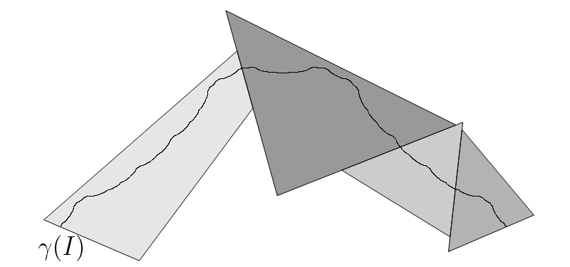 Figure 1
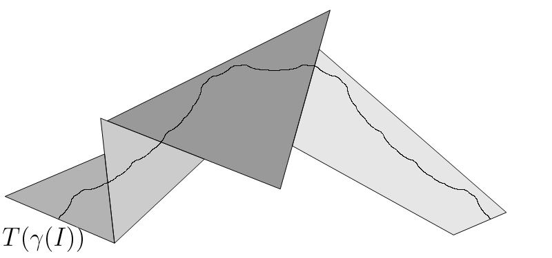 Figure 2