Dynamics of the quark-antiquark interaction and the universality of Regge trajectories
A.M. Badalian, B.L.G. Bakker

TL;DR
This paper investigates the quark-antiquark interaction in light mesons using a relativistic string Hamiltonian, demonstrating how confining potential flattening and corrections influence Regge trajectories and support their universality.
Contribution
It introduces a model incorporating flattened confining potential, self-energy, and string corrections to explain the linearity and universality of Regge trajectories in light mesons.
Findings
Both radial and orbital Regge slopes decrease by ~30% due to flattening.
Self-energy correction maintains linearity of Regge trajectories at high excitations.
Universal gluon-exchanged potential yields similar slopes for radial and orbital trajectories.
Abstract
The dynamical picture of a quark-antiquark interaction in light mesons, which provides linearity of radial and orbital Regge trajectories (RT), is studied with the use of the relativistic string Hamiltonian with flattened confining potential and taking into account the self-energy and string corrections. Due to the flattening effect both slopes, of the radial and of the orbital RT, decrease by with the value of ~GeV being larger than ~GeV. The self-energy correction provides the linearity of RT and remains important up to very high excitations; the string correction decreases the slope of the orbital RT, while the intercept GeV is equal to the squared centroid mass of . If the universal gluon-exchanged potential without fitting parameters and screening function, as in heavy quarkonia,…
Click any figure to enlarge with its caption.
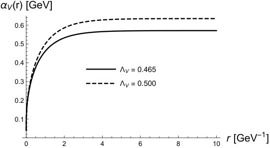 Figure 1
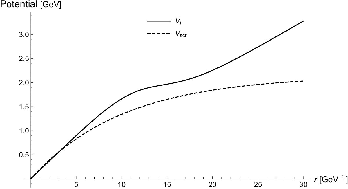 Figure 2
| Meson | |||
|---|---|---|---|
| Mass | 1689(2) | 1982(14) | 2234 |
| Meson | |||
| Mass | 1705(40) | 1995(10) | 2330(35) |
| State | |||
| 1S | 1.339 | 0.82 | 0.364 |
| 2S | 1.998 | 1.26 | 0.330 |
| 3S | 2.498 | 1.58 | 0.296 |
| 4S | 2.915 | 1.85 | 0.273 |
| 1P | 1.792 | 1.06 | 0.236 |
| 2P | 2.315 | 1.43 | 0.226 |
| 3P | 2.750 | 1.72 | 0.214 |
| 4P | 3.129 | 1.97 | 0.204 |
| 1D | 2.155 | 1.24 | 0.187 |
| 2D | 2.601 | 1.57 | 0.182 |
| 3D | 2.990 | 1.84 | 0.176 |
| 4D | 3.337 | 2.08 | 0.170 |
| 1F | 2.465 | 1.41 | 0.159 |
| 2F | 2.861 | 1.71 | 0.157 |
| 3F | 3.215 | 1.96 | 0.153 |
| 4F | 3.538 | 2.18 | 0.149 |
| State | 10 | |||||
| 1S | -0.234 | 0.405 | - 0.400 | 0 | 0.705 | 0.705(6) |
| 2S | -0.212 | 0.553 | -0.293 | 0 | 1.493 | 1.424(25) |
| 3S | -0.182 | 0.672 | -0.241 | 0 | 2.067 | 1.875(5) |
| 4S | -0.168 | 0.773 | -0.210 | 0 | 2.529 | absent |
| 1P | -0.152 | 0.486 | -0.333 | -0.044 | 1.263 | |
| 2P | -0.146 | 0.615 | -0.263 | -0.027 | 1.879 | |
| 3P | -0.138 | 0.722 | -0.224 | -0.018 | 2.369 | absent |
| 1D | -0.120 | 0.569 | -0.285 | -0.076 | 1.674 | |
| 2D | -0.117 | 0.679 | -0.238 | -0.052 | 2.194 | |
| 3D | -0.113 | 0.776 | -0.209 | -0.038 | 2.630 | absent |
| 1F | -0.102 | 0.642 | -0.252 | -0.102 | 2.009 | |
| 2F | - 0.101 | 0.741 | -0.219 | -0.076 | 2.465 | absent |
| Potential | linear CP | linear CP+ weak | linear CP+ strong |
|---|---|---|---|
| Corrections | 0 | , | |
| 0 | 0.30 | 0. 57 | |
| 1.440 | 1.225(1) | 1.13(2) | |
| 1.440 | 1.17(4) | 1.13(3) | |
| , | 1.440 | 1.12(3) | 1.09(2) |
| 2.262 | 2.14(2) | 1.97 (5) | |
| 1.696 | 0.47(1) | 0.46(2) |
| state | r.m.s (LP) | r.m.s. FCP | r.m.s. FCP+GE | (FCP) |
|---|---|---|---|---|
| 0.82 | 0.86 | 0.71 | 0.357 | |
| 1.47 | 1.53 | 1.30 | 0.288 | |
| 1.65 | 2.42 | 2.12 | 0.204 | |
| 1.78 | 2.67 | 2.61 | 0.193 | |
| 2.08 | 2.94 | 2.79 | 0.189 | |
| 1.06 | 1.13 | 1.00 | 0.226 | |
| 1.43 | 1.95 | 1.69 | 0.176 | |
| 1.72 | 2.64 | 2.53 | 0.147 | |
| 1.97 | 2.78 | 2.69 | 0.146 | |
| 1.24 | 1.41 | 1.28 | 0.172 | |
| 1.56 | 2.42 | 2.18 | 0.134 | |
| 1.83 | 2.70 | 2.67 | 0.130 | |
| 2.06 | 2.94 | 2.83 | 0.127 | |
| 1.41 | 1.77 | 1.59 | 0.134 | |
| 1.70 | 2.73 | 2.61 | 0.115 |
| 0 | 1 | 2 | 3 | |
|---|---|---|---|---|
| 1 | 0.173 | 0.167 | 0.155 | 0.150 |
| 2 | 0.162 | 0.165 | 0.150 | 0.148 |
| 3 | 0.150 | 0.158 | 0.148 | 0.146 |
| 0 | 1 | 2 | 3 | |
|---|---|---|---|---|
| 0 | 400 | 491 | 539 | 564 |
| 1 | 460 | 480 | 525 | 580 |
| 2 | 520 | 482 | 536 | 594 |
| 3 | 550 | 500 | 560 | 620 |
| State | |||||||
|---|---|---|---|---|---|---|---|
| 1339 | 0 | -405 | -225 | 66 | 775 | ||
| 1998 | -55 | -338 | -190 | 40 | 1455 | ||
| 2498 | -198 | -291 | -143 | 26 | 1892 | ||
| 2915 | -346 | -244 | -131 | 20 | 2214 |
| state | Exp. 10 | ||||
| 1792 | 0 | -140 | 1652 | ||
| 2315 | -102 | -144 | 2069 | ||
| 2750 | -278 | -123 | 2349 | absent | |
| 3129 | -398 | -114 | 2617 | absent | |
| 2155 | 0 | -124 | 2031 | ||
| 2601 | - 173 | -113 | 2315 | ||
| 2990 | -342 | -96 | 2552 | absent | |
| 3337 | -448 | -94 | 2795 | absent | |
| 2465 | 0 | -97 | 2368 | ||
| 2861 | -256 | -86 | 2519 | absent | |
| 3215 | -394 | -84 | 2737 | absent |
| state | Exp. [10] | |||||
| 1652 | 491 | - 330 | -40 | 1282 | ||
| 2069 | 480 | -310 | -33 | 1726 | ||
| 2349 | 482 | -291 | - 30 | 2028 | absent | |
| 2617 | 500 | -268 | - 25 | 2324 | absent | |
| 2031 | 539 | -292 | -77 | 1662 | ||
| 2315 | 525 | -262 | -60 | 1993 | ||
| 2552 | 536 | -257 | - 51 | 2244 | absent | |
| 2368 | 564 | -270 | - 107 | 1991 | ||
| 2519 | 580 | -231 | -80 | 2208 | absent | |
| 2737 | 594 | -221 | - 74 | 2442 | absent |
| State | Eq. (60) | Exp. | |
|---|---|---|---|
| 1282 | 1315 | ||
| 1726 | 1697 | ||
| 2028 | 2007 | absent | |
| 2324 | 2276 | absent | |
| 1662 | 1661 | ||
| 1993 | 1977 | ||
| 2244 | 2249 | absent | |
| 1991 | 1977 | ||
| 2244 | 2249 | absent | |
| 2442 | 2467 | absent |
Peer Reviews
No public reviews on file for this paper yet. If you reviewed it on a platform where reviews are public (OpenReview, ICLR, NeurIPS, ICML), you can paste yours below so the community can read it here.
Videos
No videos yet. Explain this paper in a talk, walkthrough, or lecture? Add one.
Dynamics of the quark-antiquark interaction and the universality
of Regge trajectories
A.M. Badalian
Institute of Theoretical and Experimental Physics, Moscow, Russia
B.L.G. Bakker
Faculty of Science, Vrije Universiteit, Amsterdam, The Netherlands
Abstract
The dynamical picture of a quark-antiquark interaction in light mesons, which provides linearity of radial and orbital Regge trajectories (RT), is studied with the use of the relativistic string Hamiltonian with flattened confining potential (CP) and taking into account three negative corrections: the gluon-exchanged, the self-energy, and the string corrections. Due to the flattening effect the radial slope and the orbital slope of the Regge trajectories decrease by as compared to those in linear CP, while the string correction decreases only the orbital slope by the value . The self-energy correction is very important and has large magnitude, MeV for high excitations. It also provides the linearity of the RT, built for the centroid squared masses, and gives the small value of the intercept, GeV2, equal to the squared centroid mass of . If the universal gluon-exchanged potential without fitting parameters and screening function, as in heavy quarkonia, is taken, then the radial slope, GeV, and the orbital slope, GeV2, have close values and the RT can be considered as approximately universal.
I Introduction
The spectroscopy of light mesons refers to the field where non-perturbative QCD dominates and the Regge trajectories (RT), both orbital and radial, appear to be the most explicit manifestation of non-perturbative effects. It is known that the leading RT in the ()-plane has a linear behavior with the slope GeV2, which corresponds to the value of the string tension GeV2 in the string models 1 ; 2 , and precisely this has been used in the realistic potential model with linear confining potential (CP) 3 ; 4 . Also, systematization of radial excitations of light mesons, suggested in Ref. 5 , has shown that their squared masses lie on linear, or approximately linear, radial trajectories in the ()-plane ( is the radial quantum number) and has the slope, GeV2 5 . Later in Refs. 6 ; 7 a smaller slope GeV2 was extracted from the Crystal Barrel data 8 .
It was also observed that the slopes of the ()-trajectories for the masses with spin and differ only 9 and it was assumed that within this accuracy a universal RT can exist in the -plane,
[TABLE]
with the universal slope GeV2 and the intercept GeV2. From Eq. (1) it follows that the masses of resonances with equal quantum number have to be equal and this assumption agrees with the experimental masses of the vector resonances with (see Table 1).
However, in another analysis of the experimental data, where the PDG masses and widths were used, a larger GeV2 was extracted 11 and later, after re-analysis of the experimental data, the same authors have obtained a smaller GeV2 12 with the conclusion that the universality of the radial and orbital RTs is not fulfilled at the level of 2.4 standard deviations. These results, irrespective of the fact whether slopes of radial and orbital RTs are equal or not, raise an important theoretical issue, namely, what dynamical effects are responsible for the values of the slopes, observed in experiments, and whether a universal RT exists or not. At present new studies of the RT nature continues 13 ; 14 .
A study of the light meson spectra in relativistic models shows that at first sight the RT parameters depend on the quark-antiquark potential used, but, as shown in the relativistic string model 15 ; 16 ; 17 ; 18 ; 19 ; 20 , some additional corrections to the meson masses exist. The potential was studied on a fundamental level in lattice QCD 21 ; 22 and the field correlator method 23 in the region r\mathrel{\mathchoice{\lower 3.6pt\vbox{\halign{\mathsurround=0pt\displaystyle\hfil#\hfil\cr<\crcr\sim\crcr}}}{\lower 3.6pt\vbox{\halign{\mathsurround=0pt\textstyle\hfil#\hfil\cr<\crcr\sim\crcr}}}{\lower 3.6pt\vbox{\halign{\mathsurround=0pt\scriptstyle\hfil#\hfil\cr<\crcr\sim\crcr}}}{\lower 3.6pt\vbox{\halign{\mathsurround=0pt\scriptscriptstyle\hfil#\hfil\cr<\crcr\sim\crcr}}}}1.2 fm. It was shown that in this region is the sum of the linear confining potential (CP) and the gluon-exchange (GE) term: . Precisely such a linear CP with string tension GeV2, fixed by the slope of leading angular-momentum RT, was used in the relativistic models 3 ; 4 , where a good description of the masses of low-lying states was obtained. However, to describe high excitations of light mesons, which sizes fm are large, knowledge of the quark-antiquark potential at large distances is needed, which is not defined yet on fundamental level, and in lattice QCD a flattening of the CP at r\mathrel{\mathchoice{\lower 3.6pt\vbox{\halign{\mathsurround=0pt\displaystyle\hfil#\hfil\cr>\crcr\sim\crcr}}}{\lower 3.6pt\vbox{\halign{\mathsurround=0pt\textstyle\hfil#\hfil\cr>\crcr\sim\crcr}}}{\lower 3.6pt\vbox{\halign{\mathsurround=0pt\scriptstyle\hfil#\hfil\cr>\crcr\sim\crcr}}}{\lower 3.6pt\vbox{\halign{\mathsurround=0pt\scriptscriptstyle\hfil#\hfil\cr>\crcr\sim\crcr}}}}1.2 fm is seen with large uncertainties. This flattening (screening) effect appears due to the creation of light holes (loops) in the Wilson loop and decreases the surface of the Wilson loop 17 . However, this effect was described only at a phenomenological level, assuming that a study of the high excitations can give important information about the interaction at large 15 ; 16 ; 17 .
In light mesons one can use the universal GE potential, in which the GE potential, , is now well defined at small distances, since at present the QCD constant , as well as the vector constant ) is known with a good accuracy for the number of flavours 24 . In particular, the value of MeV 24 , or the corresponding MeV 25 , appears to be larger than the value used in the past. However, the behaviour of the strong coupling at small momenta and at large distances, as in the case of the CP, is still not determined 26 and it remains unclear whether a screening GE effect exists or not. This problem will be discussed in our paper.
In Refs. 15 ; 17 it was shown that the main contribution to the light meson mass comes from the CP and as a first step it is instructive to consider the light meson spectrum, taking the purely linear CP at all distances, and after that to take into account the flattening effect and other corrections. To make the theoretical analysis more clear we consider only iso-vector light mesons with and pay special attention to calculations of the centroid masses. For that we use the relativistic string Hamiltonian (RSH), which describes the QCD string with spinless quarks at the ends and 18 ; 19 ; 20 , while the spin-dependent interaction is taken as a perturbation; in this case the instantaneous potential reduces to the linear plus the GE term.
The RSH is rather complicated and has different representations for large and small , . Its basic term , given by
[TABLE]
is well known and widely used. Its eigenvalues (e.v.s) can be approximated by an analytical expression with great accuracy, if the light quark mass . Notice that if in relativistic potential models the constituent quark mass, MeV, is used, then the parameters of the RTs depend on the value of the constituent quark mass.
The e.v. provides a basic contribution to the meson mass and for the purely linear CP the squared mass can be approximated with great accuracy by the expression 15 ; 16 ,
[TABLE]
with with the exception of . From the conventional representation of the RT as
[TABLE]
and using Eq. (3) for the purely linear CP, one obtains the following slopes and the intercept,
[TABLE]
Now the following problem arises: if the conventional value of GeV2 is taken, then all parameters of the RT (5) are significantly larger that those extracted from the experimental data 5 ; 6 ; 11 ; 12 . Namely, the orbital slope GeV2 is by larger than GeV2 of the leading RT. The radial slope GeV2 is about two times larger than the experimental GeV2 for the states with 5 ; 6 (and 1.5 times larger than for the radial trajectory), while the intercept GeV2 is 2.5 times larger than the corresponding one in Eq. (1.) Notice that the value of the intercept cannot be decreased introducing a negative (fitting) constant to the potential , as it is often done in potential models. Moreover, appearance of this constant in the mass (or potential) violates the linearity of the RT. It is important that in the RSH, used here, the potential does not contain a fitting constant.
Our goal here is to understand what effects are responsible for the strong decrease of the intercept and the slopes of the RT (5), to establish the interrelation between the parameters of the RTs and the potential , and to show the role of the string and the self-energy corrections, which are present in the mass formulas. In contrast to our previous analysis 15 ; 16 we do not assume here that a screening of the GE potential takes place at distances fm and this assumption agrees with the results of Ref. 27 , where it was shown that the screening effect of the GE potential is not seen at distances fm. We also consider how the parameters of the RT’s change for strong and weak vector coupling, taken in .
Our analysis is restricted to orbital excitations with , because high orbital excitations with have to be considered in another approximation of the RSH, where the string corrections are very large and cannot be considered as a perturbation 20 , and the ground state masses are described by the expression , in which the orbital slope of the leading RT agrees with the experimental number , if .
We pay special attention to the negative correction produced by the self-energy (SE) term 28 , which magnitude remains large, MeV, even for high excitations of light mesons; being proportional to , it provides linearity of the RT.
II The mass formulas
Here we present the structure of the mass formula, using the simplified version of the RSH, where the spin-dependent potentials, as well as the self-energy and the string contribution, are considered as a perturbation and the values of the angular momentum are restricted to 15 ; 16 . This RSH with ,
[TABLE]
is expressed via the variable , determined by the extremum condition, . It gives , i.e., is the kinetic energy of a quark. Then the Hamiltonian reduces to the form Eq. (2) and its e.v.s are defined by the spinless Salpeter equation (SSE),
[TABLE]
The e.v. is an important part of the centroid mass and for instantaneous interaction the potential is taken as the sum of confining and the GE terms,
[TABLE]
where the linear CP ,
[TABLE]
and also a flattened (screened) CP will be used,
[TABLE]
Here the function will be given in Sec. VI. The conventional form of is
[TABLE]
if there is no a screening effect, and the problem of the GE screening will be discussed in Sec. V. The contributions from the GE potential to the masses of excited states are not large, \mathrel{\mathchoice{\lower 3.6pt\vbox{\halign{\mathsurround=0pt\displaystyle\hfil#\hfil\cr<\crcr\sim\crcr}}}{\lower 3.6pt\vbox{\halign{\mathsurround=0pt\textstyle\hfil#\hfil\cr<\crcr\sim\crcr}}}{\lower 3.6pt\vbox{\halign{\mathsurround=0pt\scriptstyle\hfil#\hfil\cr<\crcr\sim\crcr}}}{\lower 3.6pt\vbox{\halign{\mathsurround=0pt\scriptscriptstyle\hfil#\hfil\cr<\crcr\sim\crcr}}}}90 MeV, nevertheless, the GE correction is very important, decreasing all parameters of the RTs.
The masses can be calculated by two ways: either solving Eq. (7) with the potential , or considering as a perturbation. It can be shown that for high excitations the exact and approximate values of mass coincide within MeV. Then in the RSH the centroid mass includes the e.v. and three negative corrections: the self-energy, the string, and ,
[TABLE]
where the self-energy correction is the largest one and three corrections together give a large negative contribution, MeV, while the e.v.s of the ground states () are the following: GeV, GeV, GeV. It is worth to underline that the centroid mass does not contain a fitting negative constant , usually introduced in potential models; this constant produces a non-linear term in the squared mass and violates the linearity of RT. On the contrary, in our approach a negative contribution from the self-energy correction,
[TABLE]
is proportional to via (see below) and therefore a non-linear term does not appear in the RT. In Eq. (13) the number depends on the quark flavour and in light mesons we take 28 . The situation is different in heavy quarkonia, where the self-energy term is small and usually neglected, since e.g. in bottomonium , GeV, and MeV. On the contrary, in a light meson has large magnitude, MeV, because the kinetic energy m.e. is small. It is important that this correction slightly decreases in higher excitations, but still remains large.
Another negative correction, the string correction , () 15 ; 16 , given by
[TABLE]
increases for states with growing and decreases for larger , however, its magnitude (in MeV) for is not large. Notice that the expression of , Eq. (14) does not change if a flattened CP is taken, but in this case the string tension has to be replaced by the averaged m.e. , which is different for every state and smaller than .
For high excitations with knowledge of the centroid mass is very important, since due to large sizes their fine-structure splitting are small and practically coincides with the masses of the members of the multiplet. It does not refer to low () states, where the spin-spin (fine-structure) splitting is not small. In particular, in the states the hyperfine correction, equal to -, with
[TABLE]
is not small even for the resonance. Calculations show that the ratio , Eq. (15), weakly depends on the parameters of the GE potential, e.g. for the ground state GeV is obtained for different types of GE potentials. This fact allows to extract from experiment with an accuracy MeV (see below).
Notice that knowledge of is of special importance since it determines the intercept of the leading trajectory (),
[TABLE]
with the intercept , where . In Eq. (15) the hyperfine correction can be determined with MeV accuracy, if the universal hyperfine coupling , the same as in heavy-light mesons and bottomonium 29 , and the theoretical number GeV is used. It gives MeV and MeV, so that the “experimental” intercept,
[TABLE]
is smaller than the intercept of the leading RT in the -plane, defined by the mass of : GeV2.
Notice that for radial excitations the difference between the squared masses, , of neighbouring states can depend on the radial quantum number . If for all states with a given the numbers are equal, then the radial RT reduces to the radial RT, introduced in Ref. 5 :
[TABLE]
where is the mass of the ground state.
III Linear confining potential
The simplest way to show the structure of the RTs is to determine the light meson spectrum in a purely linear CP and consider other interactions as a perturbation; in this case the mass is defined by analytical expressions. Notice that the linear CP plays a special role in string theory as well as in the AdS approach 30 . In a linear potential the mass formula is simplified owing to the relations,
[TABLE]
In Table 2 we give the sizes , the m.e.s , and the e.v.s , solving Eq. (7) with the linear potential with GeV2.
Knowing the m.e.s and the e.v.s , we have observed that in a purely linear CP the m.e.s can be approximated with an accuracy better than as
[TABLE]
i.e., they are proportional to . Then, with the use of the relations (19) and (20) all corrections to are given by analytical expressions.
For further analysis we rewrite the expression of (3) with GeV2,
[TABLE]
where the numbers with an accuracy better for all states, with the exception of and . Note that in (21) the slopes GeV2, GeV2, and the intercept GeV2 are significantly larger than those, extracted from experimental data 5 ; 6 ; 11 ; 12 , while due to the GE, the string, and the SE corrections the masses and the parameters of the RT decrease.
Then with the use of Eqs. (19) and (20) the orbital slope decreases owing to the string correction Eq. (14),
[TABLE]
and in the general case it depends on the quantum number : GeV2 for and GeV2 for ; for the radial RT with the slope GeV2 for and GeV2 for ; for the daughter RT with GeV and GeV2 for . Thus with the string correction taken into account the orbital slope remains large and -dependent, i.e., the RT’s can be considered as approximately linear.
III.1 The GE correction to the centroid mass
Here we take the GE potential as a perturbation and later show that exact solutions of the SSE with give a contribution to the mass, which coincides with the GE correction with high accuracy (see section VI). Using Eq. (20) the GE correction (11) can be rewritten as ()
[TABLE]
where in general the effective coupling, depends on the quantum numbers and . However, in high excitations this dependence becomes weak because of their large sizes, \mathrel{\mathchoice{\lower 3.6pt\vbox{\halign{\mathsurround=0pt\displaystyle\hfil#\hfil\cr>\crcr\sim\crcr}}}{\lower 3.6pt\vbox{\halign{\mathsurround=0pt\textstyle\hfil#\hfil\cr>\crcr\sim\crcr}}}{\lower 3.6pt\vbox{\halign{\mathsurround=0pt\scriptstyle\hfil#\hfil\cr>\crcr\sim\crcr}}}{\lower 3.6pt\vbox{\halign{\mathsurround=0pt\scriptscriptstyle\hfil#\hfil\cr>\crcr\sim\crcr}}}}1.4 fm, and the m.e.s are practically equal for all states, with the exception of the and ground states, for which the asymptotic freedom (AF) behavior of the coupling is important (see below). For other states, the values of appear to be only smaller than the asymptotic coupling . Therefore, for high excitations one can put . A typical , used in relativistic models, lies in the range, 0.55-0.63 3 ; 4 ; 16 . This value was also derived on a fundamental level 23 ; 25 ; 26 , where the uncertainty depends on the values of the vector QCD constant and the infrared (IR) regulator taken (see Section V). With the Coulomb constant and using the factor (20), one can see that
[TABLE]
is proportional to the e.v. . It means that the GE correction gives a negative contribution to all parameters of the RT: the slopes , and the intercept. Then the mass with the GE correction taken into account is
[TABLE]
but for the states
[TABLE]
where and the quantities are larger than with . From Eq. (25) one can see that the parameters of the RTs can depend on the quantum numbers through the factor , but in high excitations this dependence is weak because the term is small even for a strong GE potential. We choose the Coulomb constant, (or ) (see below) and define the average . Then for one finds and . For with , the factor is larger; for the daughter RT with , , are obtained. We can conclude that in the linear CP due to the factor , defined by the GE correction, the orbital slope decreases by , but still remains large, GeV2. Also the intercept decreases, although its value, GeV2, is kept large for all RTs.
The GE corrections give a contribution to the kinetic energy m.e.s, denoted as , see Eq. (27), which are given in Table 3 together with the SE and the string corrections, and . From this table one can see that for the ground states their masses agree with experiment, while for the states and higher excitations the masses are larger by MeV than experimental values and the only way to decrease these masses is to take into account a flattened, or screened, CP. Note that without the SE and the string corrections the masses are larger by MeV than the experimental masses .
There exists another effect, produced by the GE potential, which increases the quark kinetic energy and for the states with this m.e. can be approximated (with an accuracy better than ) by
[TABLE]
The kinetic energy is larger than and has to be taken into account in the self-energy and the string corrections, which decrease due to this effect. In some cases, instead of the approximation (27), one can use another approximation for ,
[TABLE]
III.2 The string correction
With the use of the modified kinetic energy (28) the string correction, proportional to (13), can be written as
[TABLE]
i.e., it is proportional to and contributes only to the orbital slope , decreasing its value. Since the string correction is not large ( MeV for the state, MeV, MeV, respectively, for the and ground states, and smaller for radial excitations (see Table 3), it decreases the orbital slope only by . Nevertheless, taking into account the string correction improves the agreement of the theoretical with the experimental value GeV2 11 .
III.3 The self-energy correction
The SE correction (13) is of special importance in light mesons and with the modified kinetic energy Eq. (27) can be rewritten as
[TABLE]
being proportional to . Therefore, produces a negative constant in the squared mass and strongly decreases the intercept, but does not change the radial and orbital slopes.
In Table 3 the centroid mass (10), the corrections , defined by the Eqs. (24), (29), and (30), are given together with the averaged kinetic energy (27) and the experimental values of , which are known, if the experimental masses of all members of a multiplet are measured. In the cases where in the PDG 10 only the mass of the highest state with is given, then an inequality takes place. For illustration we have chosen the vector coupling equal to a constant, , or , and neglected the asymptotic freedom (AF) effect.
In a more realistic case one can take , i.e., , for all states (with exception of the states , and ); then and the expression of the centroid mass is simplified to
[TABLE]
Than the squared mass has a clear structure,
[TABLE]
From Eq. (32) several conclusions can be drawn. One can see that the corresponding RT is non-linear through the terms and , however, taking the averaged for a given , the radial RT’s can be considered as approximately linear.
In the radial slope the GE correction ( is fixed) is defined by ,
[TABLE]
and the value GeV2 remains large for any , being larger than the experimental radial slope, GeV2 () 5 ; 6 ; 7 , even if the strong GE potential is used. Just owing to the large radial slope the large masses , given in Table 3, are obtained.
In this table we give , calculated with , which is smaller than , and in this case is MeV larger than ; is larger by MeV than , and is larger than by MeV. These masses would be only MeV smaller, if the larger was used.
The orbital slope decreases owing to both the GE and the string corrections and with ,
[TABLE]
where for large and the contribution from , which was neglected in Eq. (34), can be not small.
For the leading Regge trajectory (LRT) with the orbital slope ( ) GeV2 is in good agreement with the experimental value GeV2 7 ; 11 . However, in a daughter RT, e.g. with () the orbital slope GeV2 is by larger than and this RT is not parallel to the LRT.
From Eq. (32) one can see that the contributions to the intercept come from the GE and self-energy corrections. For the LRT the intercept GeV2 was already determined from the experimental value of , while in the orbital RT with () a cancellation of two terms occurs,
[TABLE]
and the calculated intercept agrees with the experimental intercept, GeV2, within the accuracy of the calculations.
Thus we conclude that in the purely linear CP with all corrections taken into account and large Coulomb constant, , the masses of the ground states agree with experiment, while the masses of first excitations exceed the experimental values by MeV.
IV The leading Regge trajectory
The leading RT describes the ground states with , where the , , and states have relatively small sizes (see Table 2), so for them the use of the linear CP can be justified. In the -plane () the LRT can be written as GeV2, or in the -plane it can be rewritten similar to that for (16),
[TABLE]
where the intercept is larger than the intercept GeV2 = 0.50(1) GeV2 (17).
To determine the intercept of the LRT it is not sufficient to take into account the self-energy correction, otherwise in a purely linear CP (with GeV and MeV) one would obtains the mass GeV ( GeV2), which is even larger than the experimental mass of the meson. As was shown in last section, owing to the GE potential, the kinetic energy increases from the value GeV to ÷ GeV= 0.405(10) GeV, where the uncertainty depends on the uncertainty in the QCD vector constant taken (see Table 4 and Sec. VI), and the value of GeV is obtained from the exact solutions of the SSE (7).
With GeV the self-energy correction, GeV, decreases, being MeV smaller than that for .
In the LRT the effective constants are not equal for all states, since the AF effect decreases for the and states by , while for the states with their couplings are practically equal to the asymptotic coupling .
It is of interest to notice that the coupling can be extracted from experiment, if one uses the ”experimental” value of the centroid mass, GeV (17). Taking GeV, GeV, and the mass given by
[TABLE]
one determines the effective constant (here GeV), or the effective coupling, , with a theoretical error . Note that the lower limit of , which appears to be significantly larger than , used in our paper before 15 . At the same time the upper limit of this coupling, equal to 0.51, is smaller than , used in high excitations, confirming the influence of the AF effect.
For the ground state from Eq. (20) one has and with the fitted value ( GeV), one obtains the factor , or
[TABLE]
i.e., the factor decreases the squared mass (37) by and provides the correct value of the intercept, GeV2. In the ground states with the GE correction (24), proportional to ,
[TABLE]
in general contains different values of and
[TABLE]
Then the centroid mass can be rewritten as,
[TABLE]
if the approximate relation , following from the Eqs. (27) and (28), is used, then the squared mass is
[TABLE]
Here, in the orbital slope the constants are different for the and the ground states with , for which the asymptotic value, can be used, while due to the AF effect the coupling has a value close to that for the state and here we take and . Then with and the average, , and from the Eq. (42) the orbital slope is
[TABLE]
which agrees almost precisely with experimental slope, 7 .
Also with the chosen constants and the intercept, GeV2, is obtained in good agreement with the experimental number, , where a contribution from the squared correction GeV2 is .
In Table 3 for simplicity we give the centroid masses with equal Coulomb constant, , and the masses MeV, MeV, MeV (without fine-structure splitting) turn out to be in good agreement with the experimental masses of , and (its mass, MeV) 10 ). This agreement indicates that in the ground states with the fine-structure splittings are not large. Notice that the magnitudes of the string corrections, which are equal to MeV, MeV, and MeV, for , respectively, grow for increasing .
In conclusion in Table 4 we give the parameters of the RT’s for different types of the potential : for the purely linear CP, the linear CP + weak , and for the linear CP+strong .
Thus, our analysis of the RTs, when the CP is linear at all distances and the SE, the string and the GE contributions are taken as a perturbations, has allowed to get analytical expressions for the masses and the parameters of the RTs, which have several characteristic features:
The radial slope, GeV2 (), remains larger than GeV2 by , irrespective to the strength of the GE potential used, and the cases with and were compared. 2. 2.
On the contrary, the orbital slope of the LRT GeV2 agrees with the experimental value, if the strong vector coupling is taken. This choice of the coupling is preferable, since for small coupling, , the orbital slope GeV2 and the mass of is larger than in experiment. 3. 3.
In the linear CP the orbital slope of the daughter RTs () is by larger than GeV2, even if the strong GE potential is used. Precisely for that reason the interaction has to be modified at large distances. 4. 4.
The largest effect from the GE potential refers to the masses of the states, which increases the radial slope of the - trajectory (see section VI).
V The gluon-exchange potential at large distances
Here we use the conventional potential as a simple sum, Eq. (8). This representation is confirmed by the Casimir scaling effect, observed in lattice QCD 31 and derived in the field correlator method 32 . Meanwhile, this choice as the sum of two terms does not imply that each term, the CP and the GE potentials, is described by the simple expression as in Eqs. (9) and (11) at all distances. Moreover, in lattice QCD the linear behavior of the CP is proved to be valid only in the region r\mathrel{\mathchoice{\lower 3.6pt\vbox{\halign{\mathsurround=0pt\displaystyle\hfil#\hfil\cr<\crcr\sim\crcr}}}{\lower 3.6pt\vbox{\halign{\mathsurround=0pt\textstyle\hfil#\hfil\cr<\crcr\sim\crcr}}}{\lower 3.6pt\vbox{\halign{\mathsurround=0pt\scriptstyle\hfil#\hfil\cr<\crcr\sim\crcr}}}{\lower 3.6pt\vbox{\halign{\mathsurround=0pt\scriptscriptstyle\hfil#\hfil\cr<\crcr\sim\crcr}}}}1.2 fm, while for fm, the flattening, or screening, of the CP is seen, but the details of are not studied yet and the flattened CP was only introduced phenomenologically in several models 15 ; 33 ; 34 .
Also the expression of the GE potential (11), taken from perturbative QCD, in a strict sense is valid only up to the momentum q^{2}\mathrel{\mathchoice{\lower 3.6pt\vbox{\halign{\mathsurround=0pt\displaystyle\hfil#\hfil\cr>\crcr\sim\crcr}}}{\lower 3.6pt\vbox{\halign{\mathsurround=0pt\textstyle\hfil#\hfil\cr>\crcr\sim\crcr}}}{\lower 3.6pt\vbox{\halign{\mathsurround=0pt\scriptstyle\hfil#\hfil\cr>\crcr\sim\crcr}}}{\lower 3.6pt\vbox{\halign{\mathsurround=0pt\scriptscriptstyle\hfil#\hfil\cr>\crcr\sim\crcr}}}}1.5 GeV2 in momentum space, or down to very small distances, fm in coordinate space 35 ; 36 . Therefore, to use in coordinate space in the whole region, one must first regularize the vector coupling in momentum space and then regularize by using in Eq. (47) (see below) the regularized . Notice that the asymptotic values of are equal in momentum and coordinate space 36 . It seemingly supports the idea that the OGE and confining interactions are not independent.
Here we follow the detailed analysis from Ref. 27 , which reveals at least three important effects, which can modify and owing to background fields.
The gauge invariance of the gluon exchange in the confining background requires the propagating gluon to be inside the confining film (the surface, filled by the background fields), connecting the and trajectories. The resulting area of the film should obey the Wilson minimal-area law 27 . 2. 2.
The propagating gluon can create (gluon-gluon) loops in the confining film only in the higher orders, which introduces a new mass parameter 37 , expressed via the string tension, and its value, , defined with accuracy, enters in the evolution equation together with , making the coupling dependent on the variable 16 ; 37 . 3. 3.
If the confining string is long, it can create light holes in the confining film, thus decreasing the surface of the Wilson loop (i.e., the film surface). A finite density of this holes gives rise to the flattening of the confining potential at large and due to the flattening effect the masses of high excitations decrease, since their effective string tension is smaller for large than that in the region fm 15 ; 16 .
The points 2 and 3 were discussed in the literature, while the properties of the GE interaction needs some comments and the behaviour of at large distances, called the color Coulomb screening effect, was studied first in Ref. 38 and recently in Ref. 27 .
In the simplest treatment 38 a deformation of the confining film, owing to propagating the quark and the antiquark trajectories, was not optimal and due to the transformation of a gluon into a one-gluon glue lump 23 , the screening of the GE interaction, , was shown to exist already at distances fm. Notice that such a strong screening is not seen in bottomonium, where and have sizes fm and 0.7 fm 25 ; 39 .
In a more accurate treatment 27 one has to maintain full gauge invariance of the OGE interaction, and in addition take into account the Wilson criterium of the minimal area law of the resulting film surface, which contains both OGE and confinement. Denoting the time distances between consequent gluon-exchanges as , at large , one can consider this system as a hybrid excitation of the system of size . Then, the mass of a transverse excitation is 40 . On the other hand, the average value of enters into the action (the total Lagrangian) exponent as , or . As a result one obtains an estimate of the screening mass (if ) 27 ,
[TABLE]
Note that this estimate refers to large distances, r\mathrel{\mathchoice{\lower 3.6pt\vbox{\halign{\mathsurround=0pt\displaystyle\hfil#\hfil\cr>\crcr\sim\crcr}}}{\lower 3.6pt\vbox{\halign{\mathsurround=0pt\textstyle\hfil#\hfil\cr>\crcr\sim\crcr}}}{\lower 3.6pt\vbox{\halign{\mathsurround=0pt\scriptstyle\hfil#\hfil\cr>\crcr\sim\crcr}}}{\lower 3.6pt\vbox{\halign{\mathsurround=0pt\scriptscriptstyle\hfil#\hfil\cr>\crcr\sim\crcr}}}}1 fm, where the deformation of the surface, due to the gluon exchange, is significant, while the screening (and deformation) is suppressed for the smaller .
We may conclude that the flattening of the CP and the screening of start at approximately the same distances, fm, but their nature is different. The flattening effect appears due to creation of light holes, which, decreasing the film surface (or the Wilson loop), also decreases the string tension at large distances.
The screening of the GE potential occurs because the movement of the gluon is restricted inside the film surface and gives rise to a deformation of the film, so that due to confinement a kind of “gluon mass”, GeV, appears. Thus the analysis of Ref. 27 does not support the idea that the screening of the CP and the GE potential have the same origin and the same screening function can be used for both potentials as suggested in Ref. 33 . For that reason, here the GE potential without screening is taken, while in previous studies the small (a kind of screening) was used 15 and the GE potential with exponential screening function ( GeV) was taken in Ref. 16 .
We also assume that the light mesons can be described by the universal GE potential (11) with the same parameters as in heavy quarkonia and heavy-light mesons 25 ; 39 , where the value of the vector coupling is determined by the QCD vector constant , which is defined through the QCD constant 41 :
[TABLE]
where . For it gives
[TABLE]
In pQCD the QCD constant GeV is now known from the analysis of , where the coupling was taken as input and the matching procedure at the -quark mass () and the -quark mass () was performed 24 . Then the value MeV is obtained, which is significantly larger than that used in the past 3 . With the use of the relation (46) the value, MeV, follows and this large number has a small uncertainty. However, since the value depends on the - an -quark masses, taken at the matching points, we expect that the uncertainty may be larger and this statement is confirmed in the analysis of the bottomonium spectrum 25 , where a smaller MeV was shown to provide the best description of the bottomonium spectrum, if the IR regulator GeV is used. Here in our study of the light meson spectra the preferable value of , which does not contradict the description of the bottomonium spectrum, is MeV.
In coordinate space the strong vector coupling is expressed via the vector coupling in the momentum space 16 ; 25 ,
[TABLE]
which is taken in the two-loop approximation,
[TABLE]
with . The parameters and are taken from Ref. 16 ,
[TABLE]
where for GeV the frozen (asymptotic) coupling , or , and just this value was used in our analysis of the RTs in Sections III and IV. From Eq. (47) it can be derived that the asymptotic values of the and coincide and the behaviour of for two values of the constant, GeV and 0.50 GeV, respectively, with GeV, is shown in Fig.1.
As seen from Fig.1, the AF effect is important only for the , , and states, which sizes are \mathrel{\mathchoice{\lower 3.6pt\vbox{\halign{\mathsurround=0pt\displaystyle\hfil#\hfil\cr<\crcr\sim\crcr}}}{\lower 3.6pt\vbox{\halign{\mathsurround=0pt\textstyle\hfil#\hfil\cr<\crcr\sim\crcr}}}{\lower 3.6pt\vbox{\halign{\mathsurround=0pt\scriptstyle\hfil#\hfil\cr<\crcr\sim\crcr}}}{\lower 3.6pt\vbox{\halign{\mathsurround=0pt\scriptscriptstyle\hfil#\hfil\cr<\crcr\sim\crcr}}}}1.1 fm, and the following effective coupling, are defined:
[TABLE]
As shown in Sect. III, the use of the effective coupling allows to present the physical picture in a clear way and for excited states provides the values of , given in Table 3, with accuracy MeV.
VI The flattened potential
In the flattened CP the string tension depends on ,
[TABLE]
where is defined by three parameters: first, the characteristic distance fm, where the flattening effect starts and string breaking becomes possible; its value is taken from the lattice calculations 22 . The second parameter, , determines the derivative of and the asymptotic value of the string tension,
[TABLE]
The variation of the parameter in the range (0.30-0.50) has confirmed the result of Ref. 16 that provides the best description of the spectrum (see Fig. 2, where the flattened CP is shown for ).
The third parameter, the constant , enters the function ,
[TABLE]
where at the point shows how fast the increasing function is approaching its asymptotic value, , at large distances, fm. In other aspects can be rather arbitrary.
In our analysis all parameters were varied in wide ranges: , , GeV fm, for which GeV2. The best description of the spectrum is reached for the parameter values
[TABLE]
From the physical point of view it is important that at large distances the chosen potential, becomes again linear with small and therefore provides a quark and anti-quark to be confined in a meson. This property of the flattened CP differs from that of a screened CP , used in many papers 33 ; 34 ; 42 ,
[TABLE]
which has a linear behavior with large string tension GeV2 at fm and then the screening effect starts already at fm. At large distances is approaching a constant, GeV and therefore the quark and antiquark inside a meson are not confined. The behaviour of is compared with in Fig. 2. Notice that the screening function cannot be used in the GE potential, since it produces the interaction , in which the main term, proportional to with very large Coulomb constant , produces an unstable (unlimited) spectrum and cannot be used.
In Eq. (54) the string tension GeV2 is chosen to keep for the state the averaged string tension, GeV2, as in the purely linear CP. From our point of view the phenomenological potential represents the physical picture rather well, but it has a negative feature, namely, the non-monotonic behavior near the point , and to obtain a smooth behavior of some matrix elements, a numerical regularization is needed.
With the flattened potential the spectrum significantly changes, as compared to the linear CP. First, the sizes of the excited states increase and can reach fm even for the and states (see Table 5), although the sizes of the low states () remain not large, in particular, the r.m.s of the meson, fm (if the GE potential is present), is in good agreement with predictions in other approaches 43 and for these states the linear CP can be used. Secondly, due to the flattening effect the e.v.s can be approximated like that in Eq. (21) and for the set of parameters Eq. (54) and the squared masses with can be presented as,
[TABLE]
where in all cases and the ground states () are not included, since their masses are determined by the linear CP. In Eq. (56) one can see that the orbital and radial slopes differ by for three different values of , and the orbital slope and the radial slope increase for the smaller value of ; also the values of both slopes are significantly smaller than GeV2 and GeV2 in the linear potential. This effect mostly occurs, because in the higher excitations the averaged is smaller than the string tension GeV2. It is of interest to notice that in the case with calculated here and turn out to be very close to the values obtained in the analysis of the experimental data in Refs. 11 ; 12 .
An unexpected result refers to the intercept, which in Eq. (56) is very large, GeV2, being even larger than in the linear CP. It means that in the flattened CP the GE and the SE corrections remain very important, while the string corrections is rather small. These corrections are defined by the same general formulas Eqs. (13,14), if there the kinetic energy and are replaced by the m.e.s and , respectively. However, the relations (19) and (20) for the m.e.s and are not valid anymore and they have to be calculated in every case separately. In Table 5 we compare the r.m.s. in the linear CP with that in the flattened CP (FCP) and FCP+GE potential, and show in the FCP, with or without the GE term, the sizes of the states with strongly increase.
An interesting feature of refers to the averaged m.e.s (see Table 5) and to (see Table 6), which for excitations with coincide within accuracy (if ). Also, in the flattened CP the kinetic energies , as a function of , grow slowly and have about MeV smaller values than in the linear CP. Due to this feature the self-energy correction, proportional to , remains large, about MeV, and very important for high excitations. Also, in the presence of the GE potential the kinetic energy increases slowly, by , (see Table 7) and in some cases the difference between them can be neglected.
In the flattened CP the m.e.s are small and practically equal (for high excitations), and therefore they cannot be expressed via the factors (20) and (25). Moreover, these m.e.s are not proportional to the e.v.s and this fact changes the physical picture. To calculate the GE correction the general form has to be used, and in the string and the SE corrections the averaged string tensions, which are different in the states with different (and fixed ), have to be taken. Since the GE correction is small, the orbital and the radial slopes of the -trajectory, where , practically do not change (see their values in Eq. (56) for ):
[TABLE]
Thus, in the flattened CP + GE potential the parameters of the -trajectory appear to be only smaller than those in the purely flattened CP.
In Tables 8 and 9 besides the GE corrections, we give also the e.v.s of Eq. (7) with the linear CP and the mass shifts, produced by the flattening effect: , which are large, MeV. As seen from Eq. (57), the masses , defined without the self-energy correction, are still MeV larger than their experimental values in Table 9 and we come to the conclusion that the use of the flattened CP and the GE correction cannot provide the correct intercept, because the self-energy correction plays a dominant role to decrease its value.
In Table 8 the masses of the states (for the set of the parameters (54)) together with the mass shifts due to the flattening effect, , and all corrections, including the hyperfine correction , are given.
The masses of the states agree with the experimental values, with exception of the mass of , which value is not well established yet 10 ; notice, that the calculated mass, MeV, is in agreement with the BaBar data 44 . Taking the masses from Table 8, the slope of the trajectory,
[TABLE]
is obtained, which because of a large uncertainty can be considered to be approximately linear. Nevertheless, this radial slope is in good agreement with the experimental , if the following experimental masses: MeV, MeV, MeV, and MeV 10 , are used.
The masses of the orbital excitations are given in Table 9, where one can see that in the high excitations () the shifts due to flattening, MeV, are very large, while the GE corrections, MeV, are relatively small. However, without the SE corrections, the masses, , () exceed by MeV the experimental values.
VII The universal Regge Trajectories
In the previous section it was shown that in the flattened potential plus the GE correction, the masses are larger than the experimental values by (300-400) MeV, and other corrections have to be taken into account. The string corrections , defined by the Eq. (14), depend on the m.e.s , while the expressions, Eqs. (19) and (20), are not valid anymore and here the exact values of from Table 5 (and the kinetic energy from Table 7) are used. The values of the string correction,
[TABLE]
are given in Table 10. In high excitations they are small, MeV. On the contrary, the SE corrections remain large even in high excitations, where also the centroid masses are given. From this table one can also see that the centroid masses agree with the experimental masses, although the fine-structure splittings were not taken into account.
Then using the squared masses, the RT trajectory in the () plane () can be built,
[TABLE]
where the orbital and the radial slopes have rather close values and even coincide within the theoretical errors. However, the central value of the orbital slope of this RT (60) is smaller than that of the leading RT (43) and this difference illustrates the accuracy of our calculations with the flattened potential. In Table 11 we compare the masses of the high excitations with , described by the RT (60), and those given in Table 10. One can see that in most cases the agreement is better than 30 MeV.
We have chosen here the phenomenological flattened CP (51), but one cannot exclude that the true (“ideal”) flattened CP is different, in particular, because in our case the matching of the linear and the flattened CP is not smooth. Therefore, equal values of the radial and orbital slopes are not excluded either. However, in our analysis the calculated RT can be called approximately universal.
It is important to stress that in the flattened CP plus the GE potential with the strong coupling, , the masses of the high excitations are too large and only due to the self-energy correction correct values of the masses are obtained. Our analysis also has shown that in the flattened CP the role of the GE interaction is less important and therefore one cannot draw a definite conclusion whether at large distances a strong screening of GE potential exists, or not. This statement is supported by our result that the RT in purely flattened CP with (56) and the RT (57), where in the masses the GE correction is taken into account, have practically equal GeV2 and radial slope, GeV2.
To draw the conclusion whether the GE potential is screened or not, it is more perspicuous to study not very high excitations of light mesons, but to concentrate at lower resonances with , which sizes are not very large, fm, and where the GE correction is more important. Also the information about the GE interaction at large distances can be extracted from the study of high excitations (with ) in charmonium, or the bottomonium resonances above the threshold. Notice that in charmonium the flattening effect is smaller than in light mesons 39 , but the GE correction is larger.
VIII Conclusions
The spectrum of light mesons was studied with the use of the RSH with the flattened confining potential (FCP), taking into account the gluon-exchange (GE), the self-energy (SE), and the string corrections. We have confirmed that the flattening effect, existing due to the creation of light -pairs, produces large mass shifts, which can reach MeV for the and excitations, and the best set of the flattened potential parameters was determined. Our calculations show that agreement with the experimental values of the masses can be reached, if all corrections are taken into account, but only the self-energy correction provides the linearity of the RT.
A special accent was placed on the role of the GE potential by performing calculations with the universal GE potential without screening, like the one that is used in heavy quarkonia. Our analysis has shown that for a weak GE potential (with strong screening) it is not possible to describe the leading RT(), while the masses of high excitations weakly depend on the GE corrections. If the strong universal GE potential, as in heavy quarkonia, is taken, then the light meson masses with are described by the RT, where the values of the orbital slope, GeV2 and the radial slope, GeV2 are close, thus this RT can be considered as approximately universal and the predicted masses agree with the existing experimental data.
However, in any case the -trajectory does not belong to this RT, since their masses are strongly affected by the GE interaction and the spin-spin interaction, providing a large slope of the radial trajectory, GeV2.
The reference list from the paper itself. Each links out to its DOI / PubMed record.
- 1(1) G. Chew and S. C. Frautschi, Phys. Rev. Lett. 7 , 394 (1961); P. Collins, Phys. Rept. 1 , 103 (1971);
- 2(2) D. V. Bugg, Phys. Rept. 397 , 257 (2004); E. Klempt and A. Zaitsev, Phys. Rept. 454 , 1 (2007).
- 3(3) S. Godfrey and N. Isgur. Phys. Rev. D 32 , 189 (1985).
- 4(4) D. Ebert, R. N. Faustov, and V. O. Galkin, Phys. Rev. D 79 , 114029 (2009).
- 5(5) A. V. Anisovich, V. V. Anisovich, and A. V. Sarantsev, Phys. Rev. D 62 , 051502(R) (2000).
- 6(6) V. V. Anisovich, Phys. Usp. 47 , 45 (2004); A. V. Anisovich, D.V. Bugg, V.A. Nikonov, A.V. Sarantsev, V.V. Sarantsev, Phys. Rev. D 85 , 014001 (2012).
- 7(7) D. V. Bugg, Phys. Rev. D 87 , 118501 (2013)
- 8(8) C. Amsler et al. (Crystal Barrel Collab.), Eur. Phys. J. 23 , 29 (2002).