Finite element approximation of source term identification with TV-regularization
Michael Hinze, Tran Nhan Tam Quyen

TL;DR
This paper develops a finite element approach combined with TV-regularization to accurately recover discontinuous source terms in elliptic systems from boundary measurements, ensuring stability and convergence.
Contribution
It introduces a finite element discretization for TV-regularized source identification and proves the convergence and stability of the proposed algorithm.
Findings
The method is stable and convergent.
Numerical experiments validate theoretical results.
Abstract
In this paper we investigate the problem of recovering the source term in an elliptic system from a measurement of the state on a part of the boundary. For the particular interest in reconstructing probably discontinuous sources, we use the standard least squares method with the total variation regularization. The finite element method is then applied to discretize the minimization problem, we show the stability and the convergence of this technique. Furthermore, we have proposed an algorithm to stably solve the minimization problem. We prove the iterate sequence generated by the derived algorithm converging to a minimizer of the regularization problem, and that convergence measurement is also established. Finally, a numerical experiment is presented to illustrate our theoretical findings.
Click any figure to enlarge with its caption.
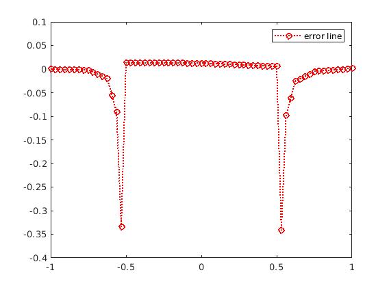 Figure 1
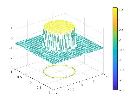 Figure 2
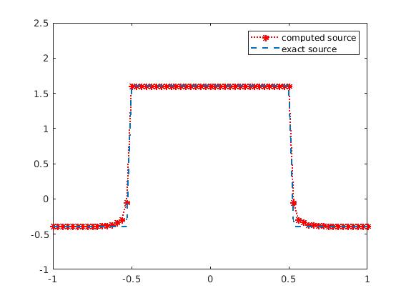 Figure 3
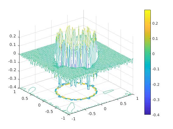 Figure 4
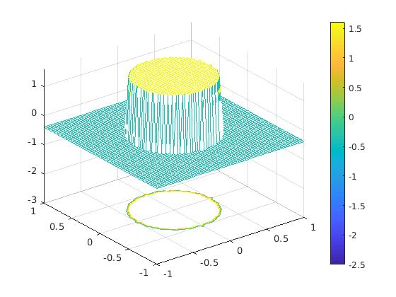 Figure 5
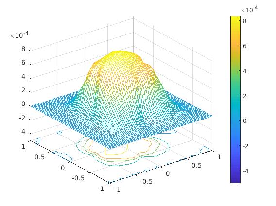 Figure 6
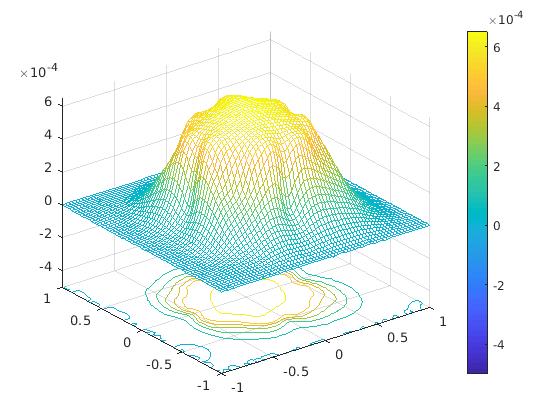 Figure 7
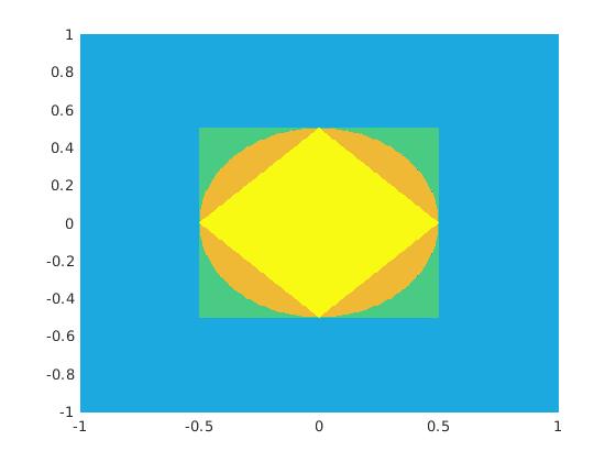 Figure 8
| Iterate | Tolerance | ||||
|---|---|---|---|---|---|
| 4 | 0.7071 | 8.4090e-4 | 2.3763e-2 | 152 | -4.0518e-6 |
| 8 | 0.3536 | 5.9460e-4 | 8.8717e-3 | 264 | -2.8826e-7 |
| 16 | 0.1766 | 4.2045e-4 | 2.5872e-3 | 343 | -1.4460e-8 |
| 32 | 8.8388e-2 | 2.9730e-4 | 1.1817e-3 | 471 | -1.1382e-7 |
| 64 | 4.4194e-2 | 2.1022e-4 | 5.6112e-4 | 561 | -4.6128e-8 |
| 4 | 0.6829 | 1.5022e-2 | 3.9121e-2 |
|---|---|---|---|
| 8 | 0.3506 | 8.5904e-3 | 3.3448e-2 |
| 16 | 0.1692 | 3.2470e-3 | 2.2919e-2 |
| 32 | 0.1095 | 1.2926e-3 | 1.5372e-2 |
| 64 | 0.7403e-2 | 6.0377e-4 | 1.2252e-2 |
Peer Reviews
No public reviews on file for this paper yet. If you reviewed it on a platform where reviews are public (OpenReview, ICLR, NeurIPS, ICML), you can paste yours below so the community can read it here.
Videos
No videos yet. Explain this paper in a talk, walkthrough, or lecture? Add one.
Finite element approximation of source term identification with TV-regularization
Michael Hinzea††Email: [email protected] [email protected] Tran Nhan Tam Quyenb,∗††∗Corresponding author
aDepartment of Mathematics, University of Hamburg, Bundesstr. 55, 20146 Hamburg, Germany
bInstitute for Numerical and Applied Mathematics, University of Goettingen, Lotzestr. 16-18, 37083 Goettingen, Germany
Abstract: In this paper we investigate the problem of recovering the source in the elliptic system
[TABLE]
from an observation of the state on a part of the boundary , where the functionals and are given. For the particular interest in reconstructing probably discontinuous sources, we use the standard least squares method with the total variation regularization, i.e. we consider a minimizer of the minimization problem
[TABLE]
as reconstruction. Here denotes the unique weak solution of the above elliptic system which depends on the source term , is the total variation of , is the regularization parameter, the admissible set with , being given constants, and is the Banach space of all bounded total variation functionals. We approximate problem with piecewise linear and continuous finite elements, where denotes the corresponding finite element approximation of . This leads to the minimization problem
[TABLE]
where . We in Theorems 3.1, 3.5 provide the numerical analysis for the discrete solutions of \big{(}\mathcal{P}^{h}\big{)}, and also propose an algorithm to stably solve this discrete minimization problem, where we are lead by the algorithmic developments of [8, 49]. In particular we prove that the iteration sequence \big{(}f^{h}_{n}\big{)}_{n} generated by this algorithm converges to a minimizer of \big{(}\mathcal{P}^{h}\big{)}, and that convergence measure of the kind
[TABLE]
is satisfied. Finally, a numerical experiment is presented to illustrate our theoretical findings.
Key words and phrases: Inverse source problem, boundary observation, total variation regularization, ill-posedness, finite element method, stability and convergence, elliptic boundary value problem.
AMS Subject Classifications: 35R25; 47A52; 35R30; 65J20; 65J22.
1 Introduction
Let be an open bounded connected set of with the polygonal boundary . In this paper we investigate the inverse problem of identifying the source term in the elliptic system
[TABLE]
from a boundary measurement of the exact data , where is the unit outward normal on and is a relatively open subset of the boundary.
In the system (1.1) the Robin boundary condition j\in H^{-1/2}(\partial\Omega):=\big{(}H^{1/2}(\partial\Omega)\big{)}^{*} and special functionals are assumed to be given, where with a.e. on , with a.e. in and is a symmetric diffusion matrix satisfying the uniformly elliptic condition
[TABLE]
for all with some constant .
We start with some notations. The expressions and stand respectively for the scalar products of the Lebesgue spaces and , while denotes the dual pair (\cdot,\cdot)_{\big{(}H^{-1/2}(\partial\Omega),H^{1/2}(\partial\Omega)\big{)}}. Let
[TABLE]
where .
We assume that a.e. in or a.e. on . Then, there exist positive constants such that
[TABLE]
for all , where denotes the usual norm of the Sobolev space (cf. [41]). Thus, the expression generates a scalar product on the space equivalent to the usual one. Consequently, for each the Robin boundary value problem (1.1) defines a unique weak solution in the sense that such that the variational equation
[TABLE]
is satisfied for all . Furthermore, the estimate
[TABLE]
holds true, where and denotes the continuous Dirichlet trace operator. Recall that is compact (cf., e.g., [37, 40]) and there is a positive constant such that
[TABLE]
for all .
In case and , by the Poincaré-Friedrichs inequality (cf., e.g., [44])
[TABLE]
for some constant depending only on , the expression is a scalar product on the space which is equivalent to the usual one. Therefore, in view of Riesz’s representation theorem, for each the problem (1.1) also has a unique weak solution which is defined via the variational equation for all and further satisfied the estimate . In the sequel we thus consider the case only. All results in present paper are still valid for the case .
The inverse problem is stated as follows:
Given a boundary measurement of the exact of (1.1), find .
For this purpose and with the particular interest in reconstructing probably discontinuous sources, we use the standard least squares method with the total variation regularization, i.e. we consider a minimizer of the minimization problem
[TABLE]
as reconstruction. Here is the regularization parameter and
[TABLE]
with , being given constants. We note that the lower and upper bound imposing upon the admissible set guarantees the existence of a minimizer to (cf. [1, 12, 17, 51]).
Let be the approximation of in the finite dimensional space of piecewise linear, continuous finite elements. We then consider the discrete total variation regularized problem corresponding to which is given by the following minimization problem
[TABLE]
where . Let us point to the reader here that a discrete total variation approach with finite elements has been recently proposed for imaging in [30]. Likewise , we can show that the problem \big{(}\mathcal{P}^{h}\big{)} admits a minimizer for each . However, due to the lack of strict convexity of the cost functional, a solution of \big{(}\mathcal{P}^{h}\big{)} may be non-unique.
As is fixed, we show that every solution sequence of the problems \big{(}\mathcal{P}^{h}\big{)}_{h} has a subsequence which converges to a solution of the problem , in -norm as well as in the total variation, where (see §3, Theorem 3.1). Furthermore, in case , and is chosen in a suitable way, every sequence of solutions to \big{(}\mathcal{P}^{h}\big{)}_{h} can be extracted a subsequence that converges to a sought source with the total variation-minimizing property (see §3, Theorem 3.5). To the best of the author’s knowledge those results are new for problem \big{(}\mathcal{P}\big{)}.
For the numerical solution of problem \big{(}\mathcal{P}^{h}\big{)}, we adopt the linearized primal-dual algorithm proposed in [49]. For the convenience of the reader we in the following sketch this approach. Starting with the equation
[TABLE]
with being a bounded linear operator, the authors have considered the unconstrained minimization problem
[TABLE]
where is the given data. Due to the -dual representation approach developed by [8, 9, 10, 14], (1.8) is rewritten as a saddle-point problem
[TABLE]
where
[TABLE]
, and denotes the indicator function of the set . Using the piecewise constant finite element space , problem (1.9) is then approximated in the -space according to
[TABLE]
For the numerical solution of this problem the scheme
[TABLE]
is proposed in [49, Algorithm 1], where the parameters are chosen suitably. Furthermore, we note that the solution to the sub-problem (1.13) is given by the explicit form (see [8, 49])
[TABLE]
In our framework we consider a constrained minimization problem, i.e. the linear space in (1.11) is replaced by the bound-constrained set , with the forward operator being affine linear arising from solutions of elliptic PDEs, and data taken on a part of the boundary. With denoting the initial guess the resulting algorithm in our notation is given by
[TABLE]
with denoting the discrete adjoint state associated to , see §2 for details. We mention that the sub-problem (1.14) admits a solution (cf. Remark 4.5)
[TABLE]
where denotes the -projection on the set and is the adjoint operator of defined by
[TABLE]
for all and .
We then show in §4 that the iteration sequence admits a subsequence which converges in the finite dimensional space to an element , where satisfies the first-order optimality condition for the considered minimization problem and is a minimizer of . Moreover, we derive the identity
[TABLE]
which is to be expected for primal-dual-type algorithms by the results of e.g. [42, 49]. We note that using sparsity regularization instead of the regularization the rate is shown in [43].
Source identification appears in many practical applications, like e.g. electroencephalography, geophysical prospecting and pollutant detection. Its PDE model-based treatment attracted great attention during the last decades, where we refer to e.g. [2, 7, 16, 21, 29, 34, 48] and the references given there. Let us briefly refer to publications related to our work. In [23, 38, 39] dual reciprocity boundary element methods are used to treat inverse source problems numerically. The situation where a priori knowledge of the identified source is available, e.g. as a point source, characteristic functional or a harmonic functional, is investigated in [5, 6, 11, 36, 46, 50]. Recently, by using a so-called energy functional method combined with Tikhonov regularization the authors in [31] studied a numerical method for the source identification problem from single Cauchy data. Finite element analysis of the problem of simultaneously identifying the source term and coefficients from distributed observations can be found in [45]. For the treatment of coefficient identification problems employing -regularization techniques we refer to [15, 18, 26, 27, 28, 47].
In the present work we study the finite element approximation and algorithm development for the identification problem of a source term in an elliptic PDE from partial observations of the state on the boundary. To the best of our knowledge numerical analysis for the problem setting we consider is not yet available, although there are many contributions to the numerical and algorithmic treatment of source identification problems. The main results of our paper are contained in Theorem 3.1, where we prove convergence of the finite element discrete regularized approximations to a solution of the corresponding continuous regularized problem as the mesh size of triangulations tends to zero, in Theorem 3.5, where we establish convergence to a sought source functional when the regularization parameter approaches to zero with a suitable coupling of noise level and mesh size, and in Theorem 4.9, where we prove convergence for the iterates of our discrete algorithm.
To conclude this introduction, we briefly present the space of functionals with bounded total variation, for more details the reader may consult [3, 4, 22, 24]. A scalar functional is said to be of bounded total variation if
[TABLE]
where denotes the -norm on defined by and is the space of continuously differentiable functionals with compact support in . The space of all functionals in with bounded total variation
[TABLE]
is a non-reflexive Banach space equipped with the norm
[TABLE]
Furthermore, if is an open bounded set with Lipschitz boundary, then .
2 Preliminaries
Now we summarize some useful properties of the source-to-solution operator . First, we note that the decomposition
[TABLE]
holds, where and are the solutions to the variational equations
[TABLE]
for all , respectively. Thus, the operator is continuously Fréchet differentiable on . For each the action of the Fréchet derivative in the direction satisfies the equation
[TABLE]
Next, along with (1.1) we consider the adjoint problem
[TABLE]
which also admits a unique weak solution defined via the variational equation
[TABLE]
for all . Furthermore, for the Fréchet differential is the unique weak solution in of the variational equation
[TABLE]
Now, for all letting
[TABLE]
a computation for all shows, by (2.5) and (2.3),
[TABLE]
and so, by (2.6),
[TABLE]
We however note that the bilinear form is in general not positive definite. In fact, considering the particular case , is the unit -matrix, and , we have that , but it gives satisfying . Therefore, the cost functional of the problem is not strictly convex. Furthermore, since the -regularization term is a semi-norm on the space only, it is also not differentiable.
Lemma 2.1** ([24]).**
(i) Let be a bounded sequence in the -norm. Then a subsequence which is denoted by the same symbol and an element exist such that converges to in the -norm.
(ii) Let be a sequence in converging to in the -norm. Then and
[TABLE]
Lemma 2.2**.**
Assume that the sequence converges to an element in the -norm. Then , the sequence converges to in the -norm and converges to in the -norm as well.
Proof.
First, by Lemma 2.1, we have . Furthermore, a subsequence exists such that
[TABLE]
Since
[TABLE]
sending to , we get for a.e. in which implies that . Now, for all and we have from (1.5) that
[TABLE]
which together with (1.4) yield
[TABLE]
that deduces . Since the limit is unique, the whole sequence converges to in the -norm also. This completes the proof. ∎
Lemma 2.3**.**
The minimization problem admits a minimizer.
Proof.
The assertion follows directly from Lemma 2.1 and Lemma 2.2, therefore omitted here (see [1] for details). ∎
3 Discretization and convergence
Let be a quasi-uniform family of regular triangulations of the domain with the mesh size such that each vertex of the polygonal boundary is a node of (cf. [13, 19]). For the definition of the discretization space of the state functionals let us denote the piecewise affine, globally continuous finite element space by
[TABLE]
where consists all polynomial functionals of degree less than or equal to 1. The piecewise constant finite element space is denoted by
[TABLE]
The admissible set is discretized as
[TABLE]
Similar to the continuous case, we for each have that the equation
[TABLE]
admits a unique solution which further satisfies the estimate
[TABLE]
where the constant is independent of the mesh size . Then the problem can be discretized by
[TABLE]
which admits a minimizer for each .
Also, the adjoint state in (2.4) has the discrete version defined via the equation
[TABLE]
for all .
We now state the following result on the stability of finite element approximations. Here and in the sequel, unless otherwise stated, we indicate by a generic positive constant which is independent of the mesh size , the regularization parameter and the observation data .
Theorem 3.1**.**
Let be a sequence with and be a fixed regularization parameter. Assume that is an arbitrary minimizer of for each . Then a subsequence of \big{(}f^{h_{n}}\big{)}_{n} not relabeled and an element exist such that
[TABLE]
Furthermore, is a solution to . If the uniqueness of the solution to is satisfied, then convergence (3.4) holds for the whole sequence.
We mention that (3.4) yields the convergence in the -norm for all . In fact, this assertion follows directly from the following estimate
[TABLE]
To prove Theorem 3.1 we need the following crucial result.
Lemma 3.2**.**
[32, Lemma 4.6.]** For any fixed an element exists such that
[TABLE]
and
[TABLE]
Lemma 3.3**.**
Assume that converges to in the -norm. Then the limit
[TABLE]
holds true.
Proof.
The proof is based on standard arguments, it is therefore omitted here. ∎
Proof of Theorem 3.1.
Let be arbitrary and be generated from due to Lemma 3.2. The optimality of , yields
[TABLE]
By (3.2) and (3.6), we deduce from the last inequality that the sequence \big{(}f^{h_{n}}\big{)}_{n} is bounded in the -norm. Then, due to Lemma 2.1, a subsequence not relabeled and an element exist such that
[TABLE]
Combining this with Lemma 3.3, we arrive at
[TABLE]
here we used Lemma 3.2 (with noting ) and Lemma 3.3 in the last equation, again. Thus, is a solution to . Furthermore, replacing in (3) by , we obtain
[TABLE]
and, together with (3.8), arrive at
[TABLE]
and so that . The proof is completed. ∎
In the remaining part of this section we investigate the convergence of discrete regularized approximations to an identified source as is chosen in a suitable way depending on the mesh size and the error level of observations. Before doing so, we introduce the notion of the total variation-minimizing solution of the identification problem.
Lemma 3.4**.**
The problem
[TABLE]
admits a solution, called the total variation-minimizing solution of the identification problem.
Proof.
The assertion follows by stand arguments, therefore omitted here. ∎
Let be fixed, we denote by
[TABLE]
[TABLE]
We now show the convergence of finite element approximations to the identification.
Theorem 3.5**.**
Assume that and and be any positive sequences such that
[TABLE]
where is arbitrary and is defined by (3.10). Furthermore, assume that is a sequence satisfying
[TABLE]
and is an arbitrary minimizer of the problem
[TABLE]
for each . Then, a subsequence of not relabeled and a total variation-minimizing solution of the identification problem exist such that
[TABLE]
Furthermore, the discrete state sequence \big{(}u^{h_{n}}(f_{n})\big{)}_{n} converges in the -norm to the unique weak solution of the boundary value problem (1.1).
Proof.
By the definition of , we have
[TABLE]
where generates from , due to Lemma 3.2. We bound
[TABLE]
Using (1.5) and (3.1), we get for all that
[TABLE]
and so that
[TABLE]
Taking , by (1.4), (3.5) and (3.10), we deduce
[TABLE]
and then
[TABLE]
Combining this with (3)–(3.14), we get
[TABLE]
It follows from the last inequality and (3.12), (3.6) that
[TABLE]
and
[TABLE]
Due to Lemma 2.1 and Lemma 3.3, a subsequence of not relabeled and an element exist such that
[TABLE]
Thus, it follows from (3.17) that
[TABLE]
and so that . Furthermore, by (3.18) and (3.19), we also get
[TABLE]
for any . Therefore, is a total variation-minimizing solution of the identification problem. Now, by setting , it implies that
[TABLE]
Finally, in view of (3.1) and (1.4) we arrive at
[TABLE]
and therefore conclude that
[TABLE]
which finishes the proof. ∎
4 An iterated total variation algorithm
The aim of this section is to propose an algorithm to reach minimizers of the problem \big{(}\mathcal{P}^{h}\big{)}. We start with the following note.
Remark 4.1**.**
(i) Any can be considered as an element of , the dual space of , by
[TABLE]
(ii) The inclusion holds via the identity
[TABLE]
Lemma 4.2**.**
For each the relation
[TABLE]
holds, where
[TABLE]
and for , .
Proof.
Let be fixed. As shown in [8] that
[TABLE]
Assume that with and . We then consider with, for all and ,
[TABLE]
and deduce from (4.2), (4.4) that
[TABLE]
The subdifferential is then given by (cf. [52, Theorem 2.4.18])
[TABLE]
and so that (4.3) follows, which finishes the proof. ∎
We mention that, similar to the decomposition (2.1), for all we have
[TABLE]
where
[TABLE]
for all . Furthermore, the identity
[TABLE]
holds for all .
Lemma 4.3**.**
The functional is a solution of if and only if there exists such that
[TABLE]
where is the discrete adjoint state defined by (3.3).
Proof.
The functionals and are both convex on the convex set , an element is thus a solution of if and only if
[TABLE]
for all . Using (3.3) and (4.7)–(4.6), we get
[TABLE]
and thus deduce from (4.10) that
[TABLE]
We here consider the convex functional
[TABLE]
where is the indicator functional of the set . Then, the inequality (4.11) is equivalent to the relation
[TABLE]
Since, for all
[TABLE]
the relation (4.12) means that there exists such that
[TABLE]
for all . This together with (4.1)–(4.2) yields (4.8). Now, for all with we have from the fact defined by the equation (4.3) that
[TABLE]
which finishes the proof. ∎
Remark 4.4**.**
The system (4.8)–(4.9) is equivalent to the following inequality
[TABLE]
for all with .
In the sequel, we make use the following notation (cf. [8, 10])
[TABLE]
By the inverse inequality (cf. [13, 19]) for all , we obtain that .
Remark 4.5**.**
Due to the optimality of in (1.14), we have that
[TABLE]
for all which can be rewritten as
[TABLE]
or
[TABLE]
where denotes the -projection on the set characterized by
[TABLE]
for each .
Remark 4.6**.**
For all let be the unique weak solution of the following variational equation
[TABLE]
for all , where is defined by (4.6). Then we have for all and that
[TABLE]
Thus, by (1.4), taking , we obtain
[TABLE]
for all . Furthermore, by (1.4), (1.7) and (4.6), it holds the estimate
[TABLE]
Remark 4.7**.**
Let
[TABLE]
Then the system (4.8)–(4.9) can be rewritten in the abbreviation form
[TABLE]
Furthermore, the optimality of and due to Algorithm 1 yields that
[TABLE]
for all .
We have the following auxiliary result.
Lemma 4.8**.**
Let and . Then the system (4.21) has the form
[TABLE]
where the matrix
[TABLE]
is symmetric, positive definite.
Proof.
Using the identity (4.18), we rewrite the system (4.21) in the form
[TABLE]
which verifies the inequality (4.22), where the matrix by the equation (1.17) is symmetric. Now we show that is positive definite. For all , by the inequality (4.19), we get
[TABLE]
This together with (4.14) yields that
[TABLE]
with
[TABLE]
satisfying the relation due to (4.15), which finishes the proof. ∎
Theorem 4.9**.**
For any fixed let be the sequence generated by Algorithm 1.
(i) Then a subsequence and an element exist such that converges to in the finite dimensional space . Furthermore, satisfies the condition (4.20), i.e. for all and is thus a minimizer of .
(ii) The equation
[TABLE]
holds true, where is some norm of the finite dimensional space .
Proof.
(i) Denote , where is an arbitrary solution to and generates from , due to Lemma 4.3. Using the notations (4.20) and (4.23), we have that
[TABLE]
Talking in (4.22), we get
[TABLE]
and so that (4) yields
[TABLE]
Talking in (4.20), we have
[TABLE]
On the other hand, by (1.17), we get
[TABLE]
Combining this with (4.27)–(4), we arrive at
[TABLE]
Then for all it follows from (4.29) that
[TABLE]
Therefore, the sequence is bounded while the series is convergent. A subsequence of not relabeled and an element then exist such that
[TABLE]
Thus sending to in (4.22), we obtain
[TABLE]
for all . As a direct consequence of (4.31) (cf. Remark 4.4) we get
[TABLE]
and so that
[TABLE]
This together with Lemma 4.2 yields . Consequently, is then a minimizer to , due to (4.31) and Lemma 4.3.
(ii) It remains to show (4.24). For all we get from (4.30) that
[TABLE]
On the other hand, in view of (4.22) we have
[TABLE]
which implies
[TABLE]
or
[TABLE]
In view of (4) we get
[TABLE]
which together with
[TABLE]
imply that
[TABLE]
and so that
[TABLE]
for all . Therefore, we arrive at
[TABLE]
by (4.32). The proof is completed. ∎
5 Numerical test
We now illustrate the theoretical result with numerical examples. For simplicity of exposition we restrict ourselves to the case where in the system (1.1), and thus consider the Neumann problem
[TABLE]
with . Let denote the characteristic functional of a Lebesgue measurable set . We assume that entries of the known symmetric diffusion matrix are defined as
[TABLE]
where
[TABLE]
see Figure 1 (bottom row, right). The sought source functional in (5.1) is assumed to be discontinuous and defined as
[TABLE]
We adopt the mesh data structure of [25] to our numerical implementation. For this purpose we divide the interval into equal segments, so that the domain is divided into triangles, where the diameter of each triangle is . The Neumann boundary data in the equation (5.2) is chosen as
[TABLE]
We note that (5.1)–(5.2) is the pure Neumann boundary value problem, so and were taken such that the compatibility condition is satisfied. Let denote the unique weak solution of (5.1)–(5.2). The Dirichlet boundary data on of the problem (5.1)–(5.2) is computed by
[TABLE]
We use Algorithm 1 which is described in Section 4 for computing the numerical solution of the problem . Before doing so, we discuss the constants and appearing in (4.15). First, we can show the inequality (see, e.g., [33, §7])
[TABLE]
for all . Therefore, the constant can be chosen by . Furthermore, in the case , the following estimate provides an upper bound for .
Lemma 5.1**.**
If , then can be chosen by , i.e. for all , the estimate
[TABLE]
holds true, where and .
Proof.
Denote by \underline{S}_{d}:=\left\{\big{(}x^{\prime},\underline{\varphi}(x^{\prime})\big{)}\in\overline{\Omega}~{}\big{|}~{}x^{\prime}:=(x_{1},\ldots,x_{d-1})~{}\mbox{and}~{}\underline{\varphi}(x^{\prime})\equiv a_{d}\right\}. First, we assume that . Then, we get
[TABLE]
which implies that
[TABLE]
Multiplying this inequality by , integrating over , we obtain
[TABLE]
Likewise, denoting by \overline{S}_{d}:=\left\{\big{(}x^{\prime},\overline{\varphi}(x^{\prime})\big{)}\in\overline{\Omega}~{}\big{|}~{}x^{\prime}:=(x_{1},\ldots,x_{d-1})~{}\mbox{and}~{}\overline{\varphi}(x^{\prime})\equiv b_{d}\right\}, we also get
[TABLE]
and arrive at
[TABLE]
This implies that (5.5) is satisfied for all . By the everywhere dense property of the set in , we conclude that (5.5) is also fulfilled for all , which finishes the proof. ∎
The constant in (1.2) is taken by . With , we then can take and . As an initial approximation we choose and . In the computation below we choose and .
For observations with noise we assume that
[TABLE]
where is the matrix of random numbers on the interval . We here refer to the discussion in [20] which states that the -misfit term is well suited for this uniformly distributed noise model. However, since is a non-reflexive Banach space and the -norm is not differentiable the use of this misfit term would cause difficulties in the numerical treatment of ill-posed inverse problems.
The measurement error is then computed as \delta_{\ell}=\big{\|}z_{\delta_{\ell}}-g^{\dagger}\big{\|}_{L^{2}(\Gamma)}. To satisfy the condition (3.12) in Theorem 3.5 we take , and .
Starting with the coarsest level , we follow [35, pp. 16] in the use of the stopping criterion. Here at each iteration we compute
[TABLE]
with and and the iteration was stopped if or the number of iterations reached the maximum iteration count of .
After obtaining the numerical solution of the first iteration process with respect to the coarsest level , we use its interpolation on the next finer mesh as an initial approximation for the algorithm on this finer mesh, and proceed similarly on the refinement levels.
Let denote the functional which is obtained at the final iterate of Algorithm 1 corresponding to the refinement level . Furthermore, we denote by the computed numerical solution to the Dirichlet problem
[TABLE]
while by the solution of the equation (5.1) supplemented with the Dirichlet boundary condition \big{(}u_{j}(f^{\dagger})\big{)}_{|\partial\Omega}.
First, we consider the case where is the bottom surface of the domain , i.e. . The numerical results of this case are summarized in Table 1 and Table 2, where we present the refinement level , mesh size of the triangulation, regularization parameter , measured noise , number of iterations, value of tolerances and errors \big{\|}f^{\dagger}-f_{\ell}\big{\|}_{\Omega}, \big{\|}u^{\dagger}-u_{\ell}\big{\|}_{\Omega} and \big{\|}u^{\dagger}-u_{\ell}\big{\|}_{1,\Omega}.
We now consider the case where includes the bottom surface and the left surface of the domain , i.e. . To try obtaining an error level similar to the case where observations were taken on the bottom surface only, in (5.6) is changed to .
Computations show that the measurement noise , , the iteration stops at . Errors \big{\|}f^{\dagger}-f_{\ell}\big{\|}_{\Omega}=6.1605.10^{-2}, \big{\|}u^{\dagger}-u_{\ell}\big{\|}_{\Omega}=5.8110.10^{-4} and \big{\|}u^{\dagger}-u_{\ell}\big{\|}_{1,\Omega}=1.1164.10^{-2}.
Acknowledgements
The authors M. Hinze and T.N.T. Quyen would like to thank the Referee and the Editor for their valuable comments and suggestions which helped to improve our paper.
The reference list from the paper itself. Each links out to its DOI / PubMed record.
- 1[1] R. Acar and C.R. Vogel, Analysis of bounded variation penalty methods for ill-posed problems, Inverse Problems 10(1994), 1217-1229.
- 2[2] S. Acosta, S. Chow, J. Taylor and V. Villamizar, On the multi–frequency inverse source problem in heterogeneous media, Inverse Problems 28(2012), 075013 (16pp).
- 3[3] L. Ambrosio, N. Fusco and D. Pallara, Functions of Bounded Variation and Free Discontinuity Problems , Oxford University Press, 2000.
- 4[4] H. Attouch, G. Buttazzo and G. Michaille, Variational Analysis in Sobolev and BV Space , SIAM: Philadelphia, 2006.
- 5[5] A.El Badia, Inverse source problem in an anisotropic medium by boundary measurements, Inverse Problems 21(2005), 1487–1506.
- 6[6] A.El. Badia, T.Ha. Duong, Some remarks on the problem of source identification from boundary measurements, Inverse Problems 14(1998), 883–891.
- 7[7] G. Bao, J. Lin and F. Triki, A multi-frequency inverse source problem, J. Differential Equations 249(2010), 3443–3465.
- 8[8] S. Bartels, Total variation minimization with finite elements: convergence and iterative solution, SIAM J. Numer. Anal. 50(2012), 1162–1180.