Use of Lagrange multiplier fields to eliminate multiloop corrections
F. T. Brandt, J. Frenkel, D. G. C. McKeon, G. S. S. Sakoda

TL;DR
This paper introduces a Lagrange multiplier field method in quantum gravity and gauge theories to restrict path integrals to classical solutions, effectively eliminating multiloop corrections beyond one loop and maintaining unitarity.
Contribution
It presents a novel approach using Lagrange multipliers to reduce loop corrections in quantum field theories, with detailed analysis of gauge invariances and BRST symmetry.
Findings
Reduces multiloop contributions to one loop in quantum gravity and Yang-Mills theories.
Maintains unitarity through BRST invariance despite loop reduction.
Provides a framework for implementing background field quantization with Lagrange multipliers.
Abstract
The problem of eliminating divergences arising in quantum gravity is generally addressed by modifying the classical Einstein-Hilbert action. These modifications might involve the introduction of local supersymmetry, the addition of terms that are higher-order in the curvature to the action, or invoking compactification of superstring theory from ten to four dimensions. An alternative to these approaches is to introduce a Lagrange multiplier field that restricts the path integral to field configurations that satisfy the classical equations of motion; this has the effect of doubling the usual one-loop contributions and of eliminating all effects beyond one loop. We show how this reduction of loop contributions occurs and find the gauge invariances present when such a Lagrange multiplier is introduced into the Yang-Mills and Einstein-Hilbert actions. Moreover, we quantize using the path…
Click any figure to enlarge with its caption.
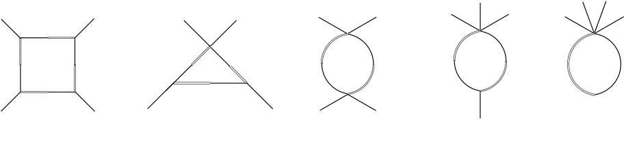 Figure 1
Peer Reviews
No public reviews on file for this paper yet. If you reviewed it on a platform where reviews are public (OpenReview, ICLR, NeurIPS, ICML), you can paste yours below so the community can read it here.
Videos
No videos yet. Explain this paper in a talk, walkthrough, or lecture? Add one.
Use of Lagrange multiplier fields to eliminate multiloop corrections
F. T. Brandt
Instituto de Física, Universidade de São Paulo, São Paulo, SP 05508-090, Brazil
J. Frenkel
Instituto de Física, Universidade de São Paulo, São Paulo, SP 05508-090, Brazil
D. G. C. McKeon
Department of Applied Mathematics, The University of Western Ontario, London, ON N6A 5B7, Canada
Department of Mathematics and Computer Science, Algoma University, Sault Ste. Marie, ON P6A 2G4, Canada
G. S. S. Sakoda
Instituto de Física, Universidade de São Paulo, São Paulo, SP 05508-090, Brazil
Abstract
The problem of eliminating divergences arising in quantum gravity is generally addressed by modifying the classical Einstein-Hilbert action. These modifications might involve the introduction of local supersymmetry, the addition of terms that are higher-order in the curvature to the action, or invoking compactification of superstring theory from ten to four dimensions. An alternative to these approaches is to introduce a Lagrange multiplier field that restricts the path integral to field configurations that satisfy the classical equations of motion; this has the effect of doubling the usual one-loop contributions and of eliminating all effects beyond one loop. We show how this reduction of loop contributions occurs and find the gauge invariances present when such a Lagrange multiplier is introduced into the Yang-Mills and Einstein-Hilbert actions. Moreover, we quantize using the path integral, discuss the renormalization, and then show how Becchi-Rouet-Stora-Tyutin (BRST) invariance can be used to both demonstrate that unitarity is retained and to find BRST relations between Green’s functions. In the Appendices we show how background field quantization can be implemented, consider the use of a Lagrange multiplier field to restrict higher-order contributions in supersymmetric theories, and derive the BRST equations satisfied by the generating functional.
gauge theories; background field method; renormalization
pacs:
11.15.-q
I Introduction
The removal of ultraviolet divergences that arise in quantum field theory has been a long-standing problem. The issue was treated systematically by Dyson Dyson:1949bp , but even then divergences arising beyond one-loop order presented special problems PhysRev.82.217 ; Collins:105730 . Renormalization to all orders is feasible only if the coupling constant is dimensionless unless symmetries that are present in the classical Lagrangian result in a cancellation between different divergent contributions. This is what makes renormalization of divergences arising when one quantizes the Einstein-Hilbert (EH) action problematic. At one-loop order, divergences are proportional to terms that vanish if the classical equation of motion for the background field are satisfied and surface terms are discarded, so a shift in the background field eliminates these divergences tHooft:1974bx ; tHooft:2002xp ; Buchbinder:1992rb , but beyond one-loop order Goroff:1986th ; vandeVen:1992gw or if the metric couples to matter fields tHooft:1974bx ; vandeVen:1992gw ; Deser:1974xq ; Deser:1974cy this shift is no longer feasible. This makes it apparent that quantization and renormalization of the gravitational field are necessarily different from the procedures that worked in electrodynamics and Yang-Mills (YM) theory.
A great deal of effort has been devoted to modifying the gravitational theory to obtain a model that is renormalizable and unitary while having General Relativity (GR) as a classical limit when in four dimensions. These attempts have met with varying degrees of success. In supergravity models, the usual generators of Poincaré symmetry are supplemented with Fermionic generators of a local gauge transformation VanNieuwenhuizen:1981ae ; Freedman:2012zz ; weinberg:book2000 . The resulting supergravity theories have improved ultraviolet behaviour PhysRevLett.38.527 , but even the most symmetric of the models (N=8 supergravity) may or may not be renormalizable PhysRevD.98.086021 , although at lower orders in the loop expansion some unexpected cancellations of divergences appear Stelle:2011zeu . In these supergravity models, there are also superparticles that have as yet been unobserved.
Another approach is to introduce into the EH action terms of quadratic or higher-order in the Riemann tensor. These terms suppress the contribution of the graviton propagator and hence can make it possible to have renormalization Stelle:1976gc . However, these propagators may now have unacceptable ghost poles, though it is possible that this shortcoming may be overcome Mannheim:2011ds . Besides, it may not be possible to reconcile these extra terms in the classical action with observations.
Treating the EH action as a low energy limit of a superstring is also a possible approach to the problem of quantizing gravity. This approach has many appealing features, but it also gives rise to several problems green_schwarz_witten_2012 ; polchinski_1998 ; west_2012 . The first quantized version of the model requires it to be defined in ten dimensions, which must be compactified in some way to dimensions. There is no fully satisfactory way of second quantizing the superstring. There is a myriad of ground states. Many as yet unobserved particles are predicted. Incorporating the Standard Model into superstring theory has not proved to be straightforward.
Loop quantum gravity Gambini:2011zz is another approach to quantizing gravity, but it too faces problems when reconciling with GR when treating a dynamical metric coupled to matter fields in the classical limit.
It has also been proposed that couplings induced by divergences that arise in the quantized EH action are “asymptotically safe” Nagy:2012ef ; that is, they approach a fixed point in the high energy limit. This has proved to be difficult to demonstrate.
If one were to simply do a canonical analysis of the EH action Dirac:1958sc ; Arnowitt:1962hi then it is difficult to obtain covariant results when using the constraint structure to quantize the theory.
We propose a relatively uncomplicated way of quantizing the EH action that makes it possible to remove divergences induced by quantum effects without losing unitarity and which retains GR in the classical limit. It involves simply introducing a term into the action in which a Lagrange multiplier (LM) field is used to ensure that the classical equations of motion are satisfied. If one quantizes a classical Lagrangian for a field that has been supplemented by such a term by using the path integral formalism, it can be shown that the one-loop radiative corrections to the classical action are twice those that occur if the term involving the LM were absent, and that all radiative effects beyond one-loop order are absent. The introduction of such an LM field has been considered in YM theory McKeon:1992rq in the Proca model Chishtie:2012hn and with the EH Lagrangian Brandt:2018lbe .
Not having any radiative effects arising beyond one-loop order simplifies the renormalization procedure needed to remove ultraviolet divergences that may arise. This is of particular relevance in dealing with the EH action; we will discuss below how all divergences (confined to one-loop order with the introduction of the LM field) can be absorbed into the LM field even when the metric interacts with matter fields.
There are precedents for considering actions in which a field occurs linearly, much like the LM field we will use. For example, Jackiw Jackiw:1984je and Teitelboim Teitelboim:1983uyTeitelboim:1983ux have provided dynamics for the metric field in dimensions by introducing a field that occurs linearly in the action; Chamseddine Chamseddine:1990hr has used this approach in conjunction with the Bosonic string. In another example, Gozzi Gozzi:1986ge has considered a path integral formulation of classical mechanics by using a LM to completely reduce the path integral to a Dirac delta function which restricts all field configuration to those satisfying the classical equations of motion. Witten Witten:1988hc has discussed the Einstein-Cartan form of the action in GR in dimensions; in this action the “dreibein” field occurs only linearly, making it possible to solve the theory. Having a fields occur only linearly in the action is also a feature of the Palatini form of the EH action in dimensions McKeon:2005be .
In the next section, we show how the introduction of a LM can be used to eliminate all loop diagrams beyond one-loop order and to double the usual one-loop contribution. This is done for an arbitrary theory, quantized using the path integral. We present both a general argument and one which employs Feynman diagrams. Next, a discussion of how the gauge symmetries, present in the original action, are affected by the introduction of the LM field and the consequences for quantization examined when using the Faddeev-Popov (FP) procedure Faddeev:1967fc .
We then apply these general considerations to the YM and EH actions. How the surviving one-loop divergences can be removed is then discussed.
An analysis of the BRST brs74 ; Tyutin:1975qk invariance of both the YM and EH actions is then considered. This approach can be used both to relate different Green’s functions and to prove unitarity in these models.
In the first appendix, we show how the use of a background field Dewitt:1967ub ; Abbott:1980hwabbott82 when quantizing modifies the LM approach. We do this as performing perturbative calculations with the EH action is only feasible if a background field is introduced. By adopting the approach of Refs. Abbott:1980hwabbott82 , we show that using the background field should not be viewed as a deficiency of a quantization procedure for GR as is sometimes stated. The background field is naturally introduced by the formalism; it is not an ad hoc entity that leaves the resulting quantized theory somehow non-covariant.
The second appendix deals with two supersymmetric models. First, the Wess-Zumino model with the LM field is considered, and then supergravity is discussed. The BRST equations are derived in a third appendix.
II The general formalism
Let us consider the action
[TABLE]
for a field . The path integral quantization procedure makes use of the generating functional
[TABLE]
In Eq. (2) we now make the replacement Brandt:2018lbe
[TABLE]
where
[TABLE]
then Eq. (2) becomes (if we set )
[TABLE]
Integration over the LM field results in a functional -function so that
[TABLE]
One can now make use of the functional analogue of the integral McKeon:1992rq ; Chishtie:2012hn ; Brandt:2018lbe
[TABLE]
where is a solution of
[TABLE]
It is the functional analogue of occurring in (7) that leads to a functional determinant appearing once the functional integral over has been performed in Eq. (6); we obtain
[TABLE]
where is a solution to the classical equation
[TABLE]
The exponential in Eq. (9) is the result of summing all tree diagrams Boulware:1968zz while the functional determinant is the square of all one-loop diagrams that arise from Eq. (5) if were absent (ie the action of Eq. (2) alone were used). No contributions beyond one-loop order arise. External fields are on shell.
This general result can be recovered using an argument that employs Feynman diagrams. If we expand so that
[TABLE]
then in Eq. (5) we find that (with symmetric)
[TABLE]
The terms bilinear in the fields , in Eq. (12) that give rise to the propagators are
[TABLE]
Since
[TABLE]
we see that there is no propagator for the field . There are, however, mixed propagators and a propagator for the for the LM field; all the vertices have at most a single LM field attached to fields. As a result, one cannot draw a Feynman diagram with more than one loop and only the field can appear on an external leg. Furthermore, only mixed propagators are allowed in the internal lines. For example, the only contributions to the four point function that follow from the Feynman rules derived from Eq. (12), are only one-loop order, and they are shown in Fig. 1. No higher loop diagrams contribute.
It can be shown that the combinatoric factor for such one-loop diagrams is always twice the one associated with the usual Feynman diagrams, when there is no LM field. As a simple example of this property, one can compare the combinatorial factors of each diagram in Fig. 1, with the corresponding ones obtained from the theory described by the action in Eq. (1). Consequently, the Feynman diagrams that follow from Eq. (12) give results consistent with the of Eq. (9).
In gauge theory models, has no inverse as it has vanishing eigenvalues; in such models the action in Eq. (1) is form invariant under the replacement
[TABLE]
In order to render the path integral of Eq. (5) well defined when this happens, we adopt the FP procedure. First though we note that if the action in Eq. (1) is invariant under (15), then
[TABLE]
and so by Eq. (16) we have form invariance if
[TABLE]
In addition, if under the gauge transformation of Eq. (15),
[TABLE]
there is form invariance if
[TABLE]
We thus see that there are now two gauge invariances associated with the action appearing in Eq. (16); there is that of Eqs. (15) and (19) as well as that of Eq. (17).
In order to eliminate the degeneracy occurring in the path integral of Eq. (5) due to these two gauge invariances, we adopt the usual FP procedure Faddeev:1967fc .
We choose to use the same gauge condition for the fields and
[TABLE]
These need not be the same; indeed it is possible to have more than one gauge condition applied to a gauge field Brandt:2007td . Next, a constant factor
[TABLE]
is inserted into the path integral of Eq. (5). The functional determinant in Eq. (31) can be rewritten in several useful ways, as
[TABLE]
with and identified with and respectively. The usual FP determinant when there is no LM is , so the result of Eq. (32a) is expected. When we discuss the BRST invariance below, Eq. (32b) is more useful; we introduce Fermionic ghost fields , , , so that
[TABLE]
where
[TABLE]
We next insert a factor of
[TABLE]
into Eq. (5). The determinant in Eq. (35) leads to the square of the usual “Nielsen-Kallosh” ghost Nielsen:1978mp ; Kallosh:1978de ; we will set and henceforth ignore it. The integrals over and in Eq. (35) can be performed using the -functions in Eq. (31) leaving us with an effective action where
[TABLE]
and
[TABLE]
In Eq. (37), and are “Nakanish-Lautrup” fields used to linearize in the gauge fixing condition of Eq. (20) and to make it possible to take the limit Nakanishi:1966zz ; Lautrup:1967zz .
We now apply these general considerations to the specific instances of the YM and EH actions.
III Yang-Mills Theory
We now will examine how the LM field can be used to reduce YM theory to one-loop order. In ref. McKeon:1992rq this was considered using the second order form of the action; here we use the first order form
[TABLE]
in which the vector potential and the field strength are treated as independent gauge fields McKeon:1994ds . Using these two field simplifies the interaction vertices in the theory. Once a LM is introduced for these two fields, is supplemented by
[TABLE]
where
[TABLE]
Since in Eq. (38) is invariant under the gauge transformation
[TABLE]
we see that by Eqs. (17) and (19) we have in addition
[TABLE]
as well as
[TABLE]
With the gauge conditions of Eq. (20) taken to be
[TABLE]
then of Eqs. (34) and (37) becomes
[TABLE]
As has the structure of Eq. (12), we see that there are no diagrams beyond one-loop order with the tree level diagrams being those that occur in normal YM theory and the one-loop diagrams being doubled. As is demonstrated in Ref. McKeon:1992rq , this means that the one-loop divergences that arise can be removed by an exact renormalization of the coupling and the wave function ; the resulting -function associated with the running of is twice the usual one-loop -function in normal YM theory.
We now turn to how the LM field can be used in conjunction with the EH action.
IV General Relativity
We now show how the LM field can be used to limit radiative effects when used in conjunction with the Palatini (first order) form of the EH action. The second order form has been considered in Ref. Brandt:2018lbe . In the first order form, only three-point vertices arise which considerably simplifies the Feynman rules that are needed.
If we use the fields
[TABLE]
where are the Christoffel symbols, then the EH action in first order form becomes in dimensions McKeon:2010nf (with )
[TABLE]
This is invariant under the infinitesimal gauge transformations
[TABLE]
which follow from diffeomorphism invariance.
LM fields and are associated with the equations of motion of and , respectively. Again using Eq. (12), we see that of Eq. (47) is supplemented by
[TABLE]
The general gauge invariances of Eqs. (15), (17) and (19) that follow from Eq. (48) are
[TABLE]
If we choose the gauge fixing conditions Nishijima:1978wq
[TABLE]
then by Eqs. (34) and (37) we find that
[TABLE]
[TABLE]
From Eqs. (47), (49), (52) and (53) it is evident that , , , , all play the role of a LM fields if one were to simply quantize the EH action of Eq. (47). Using the general arguments of section two above, we see that in any perturbative expansion of radiative effects, there are no contributions beyond one-loop order with tree effects the same as those coming from the EH action without the LM contribution and with the one-loop contributions being doubled.
The problem of having to dispose of divergences arising beyond one-loop order consequently never arises when using the LM field. The one-loop divergences vanish when the equation of motion are satisfied by the external fields (provided one discards a surface term) when one considers the EH action by itself. This means that a shift in the metric field can be used to eliminate these divergences tHooft:1974bx ; tHooft:2002xp ; Buchbinder:1992rb . The one-loop divergences that arise when the metric couples to scalar tHooft:1974bx , vector or spinor fields Deser:1974xq ; Deser:1974cy no longer are proportional to the equations of motion and hence cannot be eliminated in this way. However, in all instances the one-loop divergences are proportional to and hence they can be absorbed by in Eq. (49). Having the one-loop divergences absorbed by the LM field when considering the EH action and its extensions when the metric couples to matter fields is distinct from what happens when we considered the YM field in the preceding section. This is discussed in more detail in Ref. Brandt:2018lbe .
We now will consider how invariance under BRST transformations can be used when a LM field is introduced in a classical gauge theory.
V BRST Invariance
The well known BRST (Becchi-Rouet-Stora-Tyutin) brs74 ; Tyutin:1975qk ; Kugo:1979gm ; Nakanishi:1990qm procedure for finding a non-linear global Fermionic symmetry for the effective action in gauge theories can be adapted to the presence of a LM field. For YM theory, the effective action of Eqs. (38), (39) and (45) is invariant under the transformation
[TABLE]
where is a constant Grassmann parameter. Upon invoking the Jacobi identity, it can be verified that for each of the fields in Eq. (54), is nilpotent so that
[TABLE]
Since the effective action of Eqs. (38), (39) and (45) is invariant under this transformation, the argument of Refs. Kugo:1979gm ; Nakanishi:1990qm ; peskin_scroeder can be used to establish the unitarity of first order YM theory when supplemented with a LM field.
Much the same approach can now be used with the first order (Palatini) form of the EH action when supplemented with a LM field. The BRST transformation for the second order EH by itself has been considered in Nishijima:1978wq ; Nakanishi:1990qm ; Delbourgo:1976xd ; Nakanishi:1977gt ; Faizal:2010dw . When dealing with the effective action arising from the sum of Eqs. (47), (49), (52) and (53), we can use Eq. (54) as a guide to obtaining the appropriate BRST transformations. One can establish invariance of the effective action under the transformations
[TABLE]
If is now identified with the fields appearing in Eqs. (56), we find that once again Eq. (55) is satisfied.
Greens functions in gauge theories are not all independent because of the symmetries present Slavnov:1972fg ; Taylor:1971ff . Dealing with gauge symmetries through the BRST identities provides a straightforward way of finding these relations. In fact, if there is a LM present so that all radiative corrections are just one-loop with only gauge fields on external legs, the approach in which the LM field is absent can be easily adopted. The usual method to derive the BRST equation starts from the symmetry of the generating functional of connected Green’s functions. Then, by a Legendre transform one obtains the generating functional of the one-particle irreducible Green’s functions. We shall not repeat here this procedure, which is well known (see, for example, the chapter 7 of Ref ryder:book94 ). Instead, we will emphasize the important fact that the BRST equation directly reflects the symmetry of the gauge theory under BRST transformations. Using the YM effective action of Eqs. (38), (39) and (45) with the BRST invariance of Eq. (54), we can supplement with source terms KlubergStern:1974rs
[TABLE]
where the invariant sources , , , , and are coupled to the non-linear variations of the fields , , , , and given by Eq. (54). Notice that the variations of and are linear in the fields so that the introduction of new sources is not needed here. Due to the nilpotency (55) of these variations, we see that similarly to , is also invariant under BRST transformations. Consequently, the total action
[TABLE]
will also be invariant. This invariance under BRST transformation (54) can be expressed as
[TABLE]
Using (57), one can write (59) in the alternative way
[TABLE]
To obtain a simpler form of this equation, we note that from (58) one can verify the following useful relations involving , , and
[TABLE]
With the help of these relations, Eq. (60) becomes, after integration by parts
[TABLE]
Finally, defining a new generating functional by
[TABLE]
which has the gauge-fixing terms omitted, we obtain from Eq. (V) the BRST identities for the effective action
[TABLE]
We note that the above equation is valid to lowest order. But a similar result can be obtained to higher orders by considering all fields and sources as being bare quantities Frenkel:2017xvm and replacing the fields by their expectation values (see Appendix C). In the standard approaches taylor:1976b ; itzykson:1980b such identities have been extensively used to give an all-order inductive proof of renormalizability. In our case, where graphs beyond one-loop order are absent, the BRST identities (64) are also useful to describe the relations between the proper Green functions as well as their properties. For example, it follows from (64) that the gluon-self energy satisfies the transversality condition
[TABLE]
We have verified explicitly this relation to one-loop order.
The BRST transformations of Eq. (56) can be similarly derived from the effective action arising from the sum of Eqs. (47), (49), (52) and (53), by adding the source action (compare with (57))
[TABLE]
where the invariant sources , , , , and are coupled to the non-linear variations of , , , , and . Proceeding in parallel to the previous analysis, we find that the BRST equation for the first-order form of the EH action, when supplemented with a LM field, are given by (compare with (64))
[TABLE]
where the effective action has the gauge-fixing terms subtracted.
The BRST Eq. (67) is useful to get basic relations between the proper Green’s functions arising in quantum gravity theory with Lagrange multiplier fields. The above identities, which reflect the gauge invariance of the theory, are thus well suited to fix the structure of the counterterms. We have studied the corresponding ultraviolet contributions to one-loop order and verified that these are twice those occurring in standard quantum gravity. But as we have pointed out, there are no higher-order loop contributions in the present theory.
The above BRST identities yield precise connections between the unphysical gauge bosons polarization states and the ghost fields. Using the arguments of Refs. Kugo:1979gm ; Nakanishi:1990qm ; peskin_scroeder , one can show that these relations lead to a cancellation of the unphysical degrees of freedom in the S-matrix, which establishes the unitarity of the Lagrange multiplier theory.
VI Discussion
In this paper, we have first of all shown that if a standard classical action is supplemented with a term in which a LM field is used to ensure that the classical equations of motion are satisfied, then path integral quantization can be used to show that the usual tree level diagrams are retained, the usual one-loop diagrams are doubled and all diagrams beyond one-loop vanish.
We then show how such a LM field can be used when considering the first order form of the YM and EH actions. The Faddeev-Popov approach is employed to remove the non-physical degrees of freedom and BRST invariance of the effective actions in both cases is presented. It is argued that the BRST invariance ensures the unitarity of these theories when the LM field has been introduced.
We have explicitly verified unitarity to one-loop order in both YM and EH theories by showing that the imaginary part of the self-energy amplitudes are proportional to the corresponding cross sections calculated in the Born approximation. Since all higher loop contributions of amplitudes are suppressed, unitarity implies that all the contributions to the imaginary part of the self-energy amplitudes can be expressed just in terms of the -matrix elements evaluated in the tree approximation.
The perturbative series in usual quantum field theories may diverge even asymptotically Dyson:1952tj . However, this is not the case if a LM field is used to suppress higher loop contributions. In any case, it is generally possible to find a renormalization scheme in which higher loop calculations only serve to alter the renormalization group functions Chishtie:2015lwk .
Radiative effects arising beyond one-loop order have consequences that can be compared with experimental results when dealing with the Standard Model, so introduction of a LM field is only of academic interest when dealing with the YM field. However, the EH action for GR is non-renormalizable beyond one-loop order and loses all renormalizability when coupled with matter fields. These deficiencies are overcome if a LM field is introduced; one could consider this as a way of reconcile quantum mechanics and General Relativity without having to introduce extra dimensions, unobserved fields or break unitarity. The LM field might be seen to play a role analogous to the Higgs field in the Standard Model in that it serves to make it possible to cope with ultraviolet divergences. Unfortunately there are currently no experiments that could test this approach Donoghue:2017pgk .
Acknowledgements.
F. T. B. and J. F. thank CNPq (Brazil) for financial support. D. G. C. M. thanks Roger Macleod for an enlightening discussion and FAPESP (Brazil), Grant No. 2018/01073-5, for financial support.
Appendix A The Background field
Background fields Dewitt:1967ub ; Abbott:1980hwabbott82 , have not been introduced in the body of this paper, but without using a background field, perturbative calculations are not possible when dealing with the EH action. This has been viewed as a deficiency of using this approach to quantize the EH action that we have employed. However, we wish to demonstrate (using arguments in Refs. Culumovic:1989nw ; Brandt:2018lbe ) that the background field is not something introduced in an ad hoc manner and the presence of background fields is not a deficiency.
We begin with the path integral of Eq. (2) for the generating functional for all Feynman diagrams. Connected diagrams are generated by where Abbott:1980hwabbott82
[TABLE]
If we define
[TABLE]
and make the Legendre transform
[TABLE]
we obtain , the generating functional for 1PI diagrams. Eq. (68) can now be written as
[TABLE]
as by Eq. (70)
[TABLE]
The shift
[TABLE]
results in
[TABLE]
This shows that the background field is not just inserted by hand; it is the field associated with the current when making a Legendre transform of the generating functional for connected Green’s functions McKeon:1985uc ; Rebhan:1984bg .
We can now substitute the expansions
[TABLE]
and
[TABLE]
(which follow from Eq. (11)) into Eq. (71). This shows that
[TABLE]
Upon matching like powers of in Eq. (A), we see that
[TABLE]
From Eq. (78), it follows that
[TABLE]
and so the term in Eq. (76) that is linear in the quantum field does not contribute to because of a cancellation, not because satisfies the classical equations of motion. Higher orders in in Eq. (A) yield explicit expressions for the 1PI Green’s functions in the loop expansions Coleman:1973jx (though on occasion the loop expansion and an expansion in powers of do not match Holstein:2004dn ).
Having terms linear in cancel in (A) complicates the BRST identities to prove renormalizability of gauge theories Frenkel:2018xup ; Brandt:2018wxe . However, having a background field can be advantageous in gauge theories, as one can chose a gauge fixing condition that retains gauge invariance in the background field. Such a covariant gauge choice in YM theory is Honerkamp:1972fd
[TABLE]
with non-covariant choices considered in Ref. McKeon:1985ue . For the EH action in both first and second order form, if the background metric is and the quantum metric , then the gauge transformation of that follows from Eq. (48a) is
[TABLE]
where “” denotes a covariant derivative using the background metric . A suitable gauge choice is
[TABLE]
as this is covariant under transformations in the background field. The BRST transformation associated with the gauge choice of Eq. (82) is considered in Ref. Faizal:2010dw . The use of Eq. (82) with two different choices of the parameter in order to have a propagator for that is both transverse and traceless is considered in Refs. Brandt:2007td ; Brandt:2017oib .
Appendix B Supersymmetry
In this appendix we will show how a LM field can be used in conjunction with a Fermionic equation of motion. We first will consider the Wess-Zumino model in which there is a global supersymmetry, and then briefly examine supergravity.
We use chiral superfields 111We use the conventions , , , , , , , , , , , , , , and . ()
[TABLE]
and (with , , in Eq. (83)). The action we consider is where
[TABLE]
and
[TABLE]
If we express in terms of component fields and use the algebraic equations of motion to eliminate the auxiliary scalar fields and , then is of the form of the usual Wess-Zumino model for the spinor and the scalar with and acting as LM fields; all radiative effects are hence reduced to one-loop order as in Eq. (9).
The arguments given in Ref. Grisaru:1979wc are sufficiently general, so that these can also be used to show that is not renormalized when is added to and so we find that the renormalized quantities (, , ) are related to the bare quantities (, , ) by
[TABLE]
At one-loop order in momentum space (, in dimensions)
[TABLE]
which if
[TABLE]
then
[TABLE]
For the three-point function we find that
[TABLE]
provided , which is required if is unrenormalized.
If is to be dimensionless, then we replace by where is a dimensionful renormalization mass scale; Eq. (89) becomes
[TABLE]
so that
[TABLE]
This is an exact expression for the -function with being twice what occurs in the one-loop -function when there is no LM field in addition to the WZ field.
Supergravity is a gauge model in which supersymmetry is local. (Three reviews are in Refs. VanNieuwenhuizen:1981ae ; Freedman:2012zz ; weinberg:book2000 .) As has been noted, the EH action is renormalizable only at one-loop order if no matter fields are present. However, supergravity, even if coupled to matter superfields, is one-loop finite PhysRevLett.38.527 . Explicit higher loop calculations reveal some unexpected cancellations of divergences; it is even possible that supergravity is fully renormalizable due to the presence of some as yet unknown symmetry Stelle:2011zeu .
The introduction of a LM superfield can be used to eliminate the higher order divergences that potentially appear beyond one-loop order in a supergravity model. Consider for example supergravity with fields (the graviton, gravitino and auxiliary fields) coupled to the supersymmetric Standard Model or Grand Unified model with fields (leptons, quarks, gauge Bosons and Higgs Fayet:1976etFayet:1977yc ; Sherry:1979tb ). The two Lagrangians for these are and respectively, and the total Lagrangian is Chamseddine:1982jx
[TABLE]
is invariant under the local supersymmetry transformation
[TABLE]
and is invariant under
[TABLE]
where in (95a)
[TABLE]
We now consider the action
[TABLE]
The LM superfield in Eq. (97) is only associated with the supergravity Lagrangian. The general arguments following Eq. (13) show that the vierbein field and the gravitino field have no propagator though there is a propagator in which these fields mix with their associated LM fields. All the matter fields in have their own propagator. Vertices arising from have at most one LM field; can occur multiple times on vertices arising from and while appears only on vertices in .
We see that all diagrams with virtual contributions involving or are restricted to one-loop order and are twice those coming from alone. Virtual matter fields can occur in higher order diagrams in the loop expansion. External fields and can occur on both the one-loop diagrams coming from alone and diagrams at any order in the loop expansion coming from . All one-loop subdiagrams coming from higher order diagrams with external and are finite PhysRevLett.38.527 and so we can infer that these higher order diagrams are themselves finite. Divergences in diagrams which involve matter fields (either externally or an internal lime) can be removed through renormalization.
Quantization can proceed using the Faddeev-Popov procedure as was employed in Eqs. (20), (31), (32), (33), (34), (35), (36) and (37).
Appendix C Slavnov-Taylor identities
In this appendix we will outline the standard derivation of Slavnov-Taylor identities Slavnov:1972fg ; Taylor:1971ff . Let us consider the generating functional of (2)
[TABLE]
(Here “i” may be a continuous or discrete index; we use De Witt’s extension of the Einstein summation convention. We also consider units such that .) One can always perform a field transformation such that
[TABLE]
where is a general nonlinear functional of the fields. Then, up to first order in , we obtain from Eq. (98)
[TABLE]
Replacing the dependence inside the square bracket of (100) by acting on , we obtain
[TABLE]
The identity in Eq. (101) is a direct consequence of the independence of on field redefinitions. The simplest case occurs when is independent of so that the transformation is simply a field independent translation. (In this case we have the Dyson-Schwinger equation.) Here we are interested in the general case when there is a symmetry in the classical action, so that
[TABLE]
we also assume that the transformations do not change the path integral measure so that
[TABLE]
For these symmetry transformations, we obtain from Eq. (101)
[TABLE]
Using
[TABLE]
where is the generator of the 1PI Green’s functions, Eq. (104) can be written as
[TABLE]
Since
[TABLE]
Eq. (106) can be written as
[TABLE]
Eq. (108) shows that is invariant under
[TABLE]
(compare with (99)). In general, when is non-linear, .
Let us now add some extra source terms to in such a way that the generating functional becomes
[TABLE]
where the invariant sources are coupled to the non-linear variations of the fields. In the specific examples of the gauge theories of gravity and Yang-Mills (see section V), this excludes the variations of the anti-ghosts, which are linear. But it may be shown that such variations are cancelled by the corresponding variations of the gauge-fixing terms. Using this property, we will leave out the gauge-fixing terms as well as such variations and consider in what follows only the fields whose variations are non-linear. Using again the symmetry of and the invariance of the path integral measure, we obtain from (110)
[TABLE]
Considering the class of transformations which are nilpotent, so that and using
[TABLE]
we obtain from Eq. (111)
[TABLE]
Finally, from the Legendre transformation
[TABLE]
we have
[TABLE]
so that Eq. (113) can be written as
[TABLE]
This equation can be used to find relations between Green’s functions that follow from gauge invariance, such as those of Eqs. (64) and (67) obtained in the Yang-Mills theory and general relativity, respectively.
The reference list from the paper itself. Each links out to its DOI / PubMed record.
- 1(1) F. J. Dyson, Phys. Rev. 75 , 486 (1949).
- 2(2) A. Salam, Phys. Rev. 82 , 217 (1951).
- 3(3) J. C. Collins, Renormalization , Cambridge Monographs on Mathematical Physics (Cambridge Univ. Press, Cambridge, 1984).
- 4(4) G. ’t Hooft and M. J. G. Veltman, Annales Poincare Phys. Theor. A 20 , 69 (1974).
- 5(5) G. ’t Hooft, 249 (2002), prepared for International School of Subnuclear Physics: 40th Course: From Quarks and Gluons to Quantum Gravity, Erice, Sicily, Italy, 29 Aug - 7 Sep 2002 (this paper can be downloaded from https://www.staff.science.uu.nl/ ∼ similar-to \sim hooft 101/lectures/erice 02.pdf).
- 6(6) I. L. Buchbinder, S. D. Odintsov, and I. L. Shapiro, Effective action in quantum gravity (IOP, Bristol, UK, 1992).
- 7(7) M. H. Goroff and A. Sagnotti, Nucl. Phys. B 266 , 709 (1986).
- 8(8) A. E. M. van de Ven, Nucl. Phys. B 378 , 309 (1992).