Evaluating Quasi-Periodic Variations in the $\gamma$-ray Lightcurves of Fermi-LAT Blazars
F. Ait Benkhali (1), W. Hofmann (1), F.M. Rieger (1, 2), N., Chakraborty (1, 3) ((1) Max-Planck-Institut f\"ur Kernphysik, Germany, (2), ZAH, Institut f\"ur Theoretische Astrophysik, Universit\"at Heidelberg,, Germany, (3) Data Assimilation Research Centre, University of Reading

TL;DR
This study analyzes gamma-ray light curves of six blazars over nearly a decade to assess the presence of quasi-periodic variations, finding that apparent periodicities are not statistically significant when accounting for random variability.
Contribution
The paper provides an updated, rigorous timing analysis of multiple blazars using advanced statistical methods to evaluate the significance of quasi-periodic variations in gamma-ray light curves.
Findings
Possible year-like QPVs observed with ~3 sigma significance.
Most blazars exhibit variability consistent with log-normal distribution.
Observed periods cluster around 1.6 years, but significance is reduced globally.
Abstract
The detection of periodicities in light curves of active galacticnuclei (AGN) could have profound consequences for our understanding of the nature and radiation physics of these objects. At high energies (HE; E>100 MeV) 5 blazars (PG 1553+113,PKS 2155-304, 0426-380, 0537-441, 0301-243) have been reported to show year-like quasi-periodic variations (QPVs) with significance >3 sig. As these findings are based on few cycles only, care needs to be taken to properly account for random variations which can produce intervals of seemingly periodic behaviour. We present results of an updated timing analysis for 6 blazars (adding PKS 0447-439), utilizing suitable methods to evaluate their long term variability properties and to search for QPVs in their light curves. We generate gamma-ray light curves covering almost 10 years, study their timing properties and search for QPVs using the…
Click any figure to enlarge with its caption.
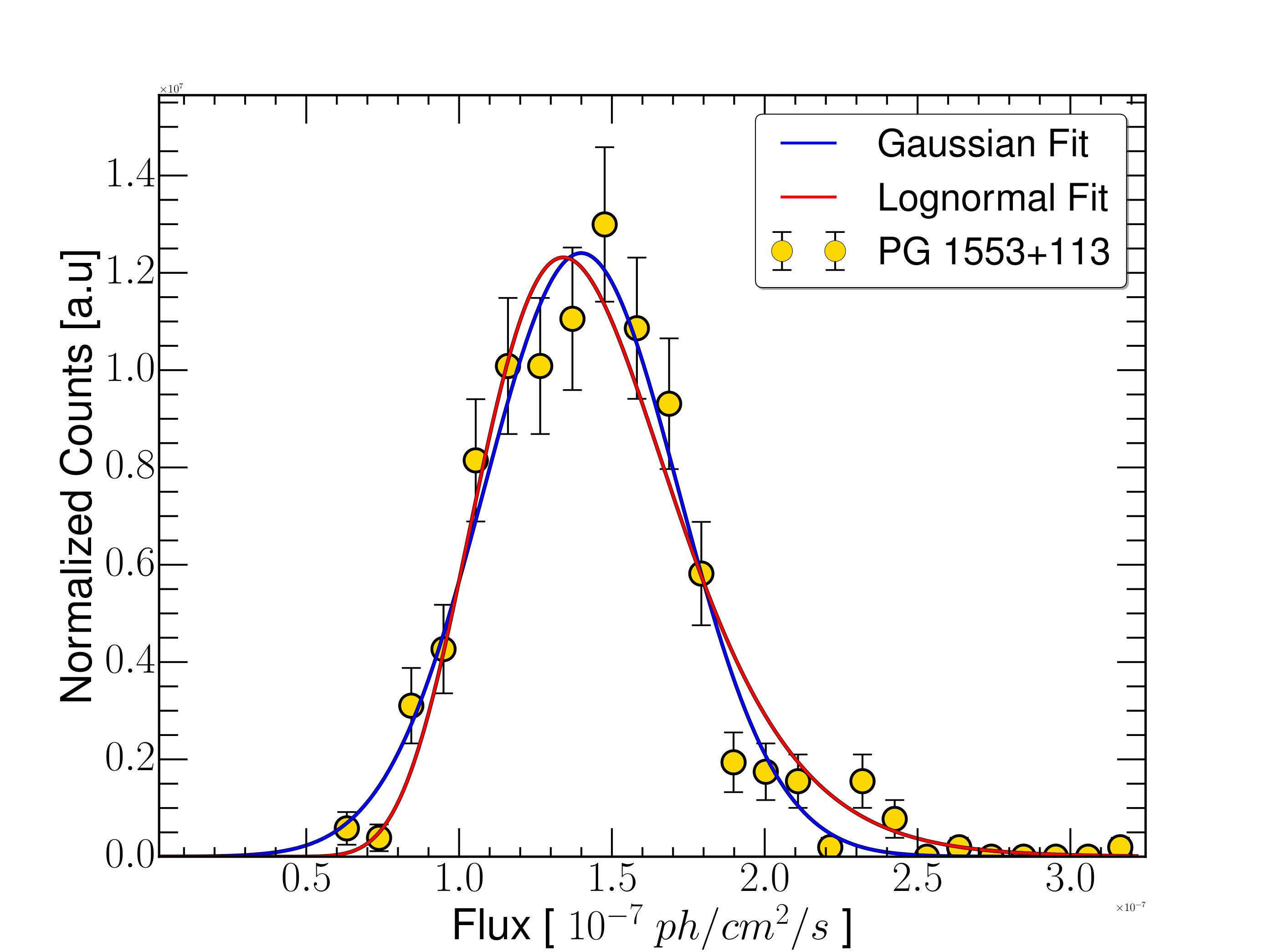 Figure 1
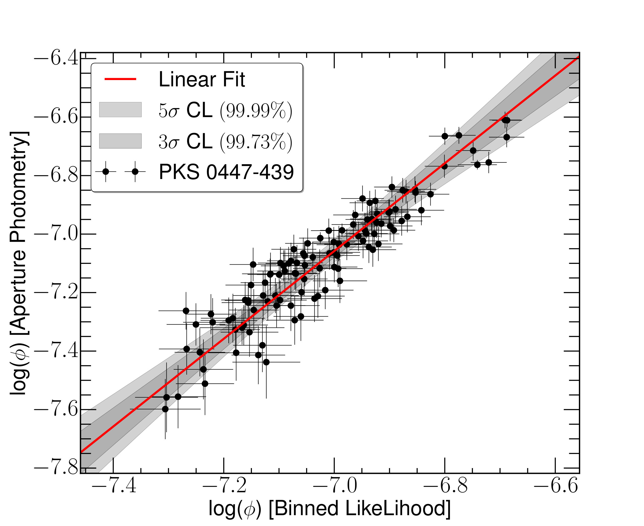 Figure 2
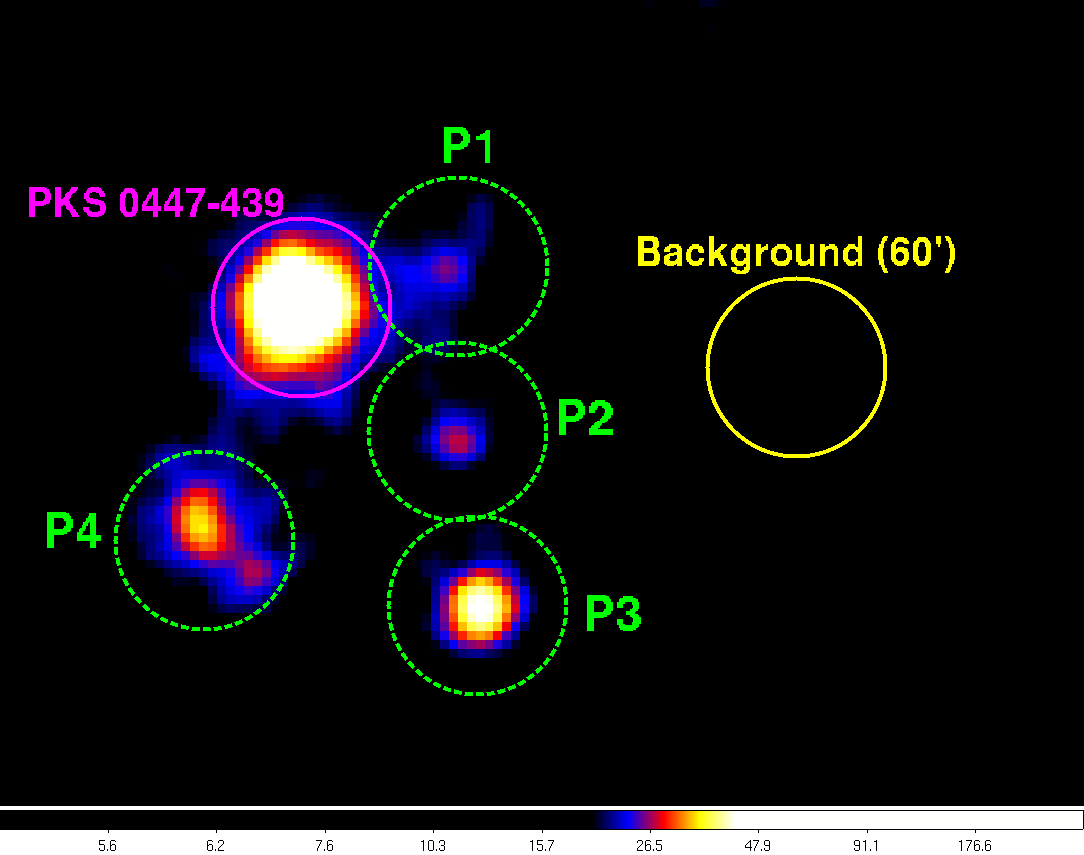 Figure 3
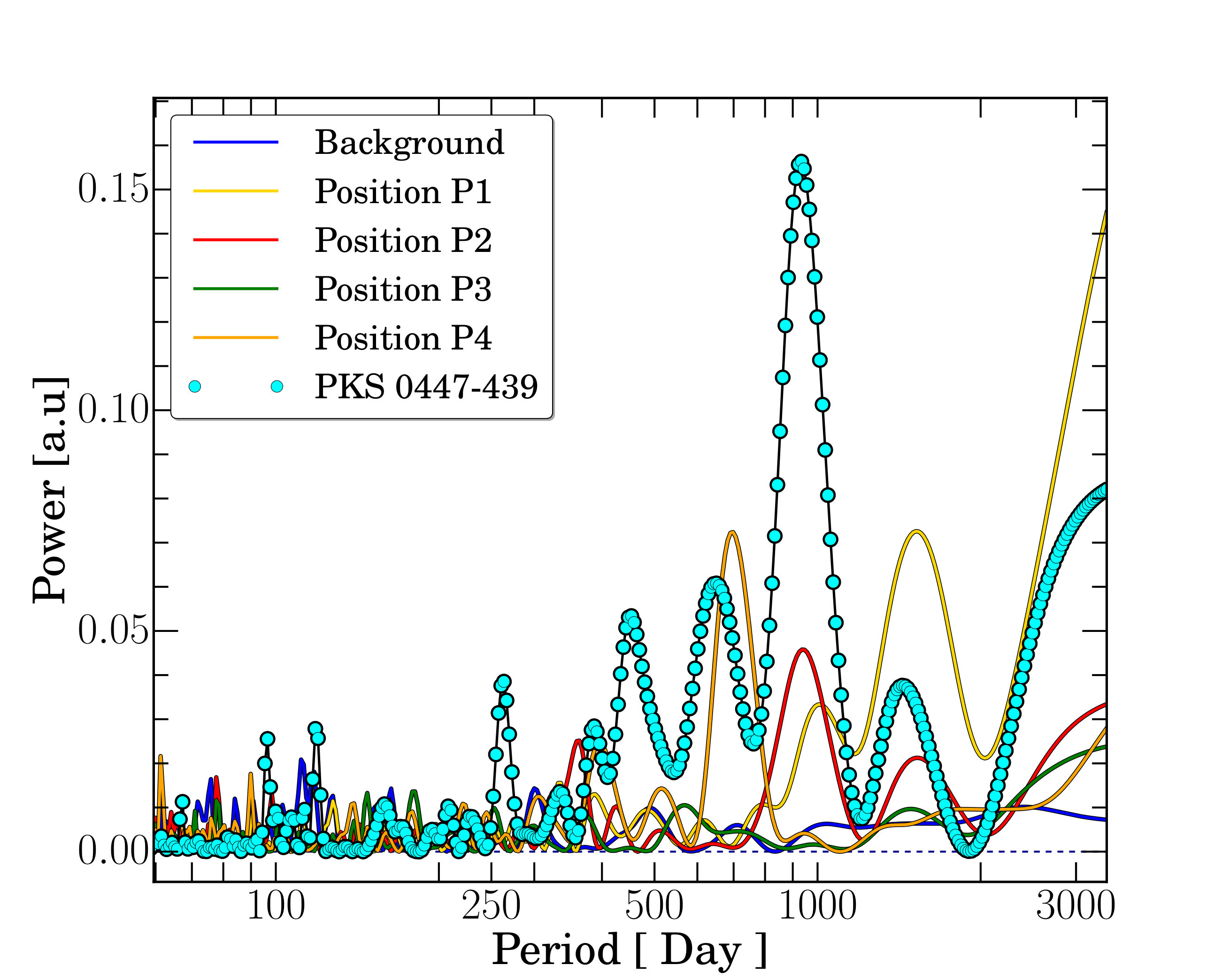 Figure 4
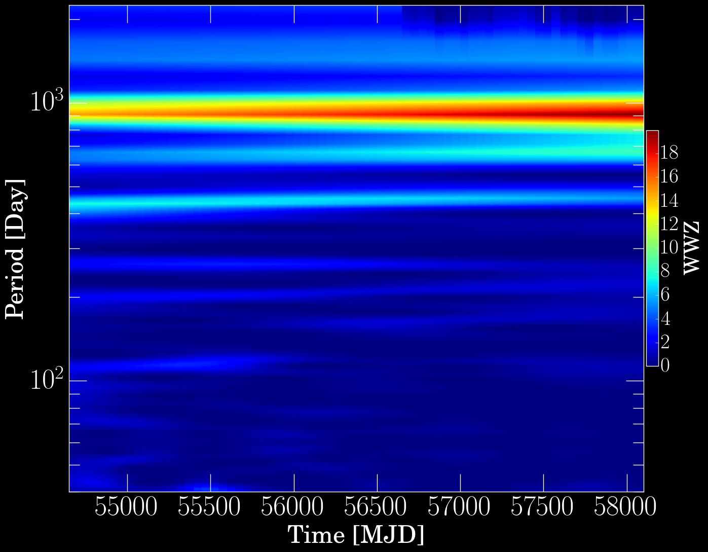 Figure 5
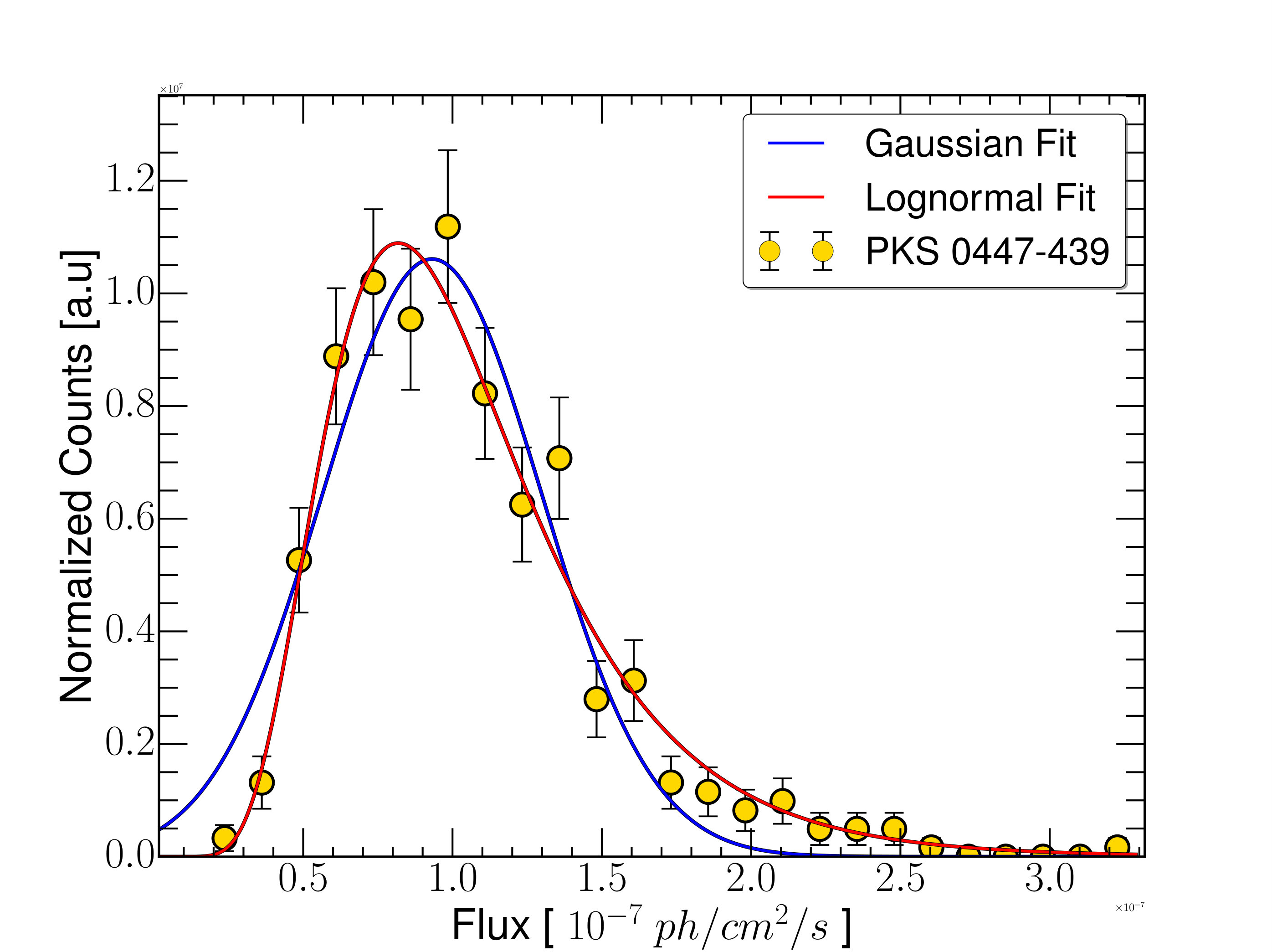 Figure 6
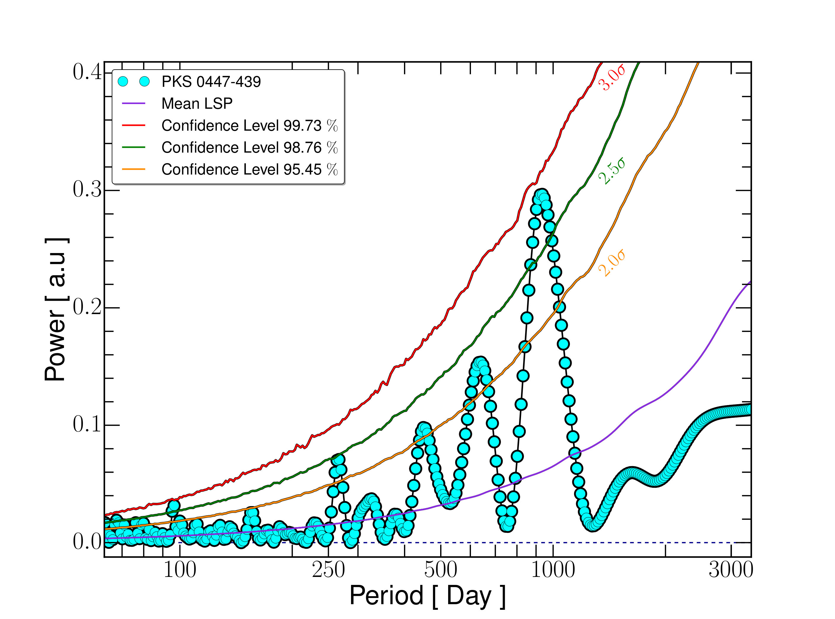 Figure 7
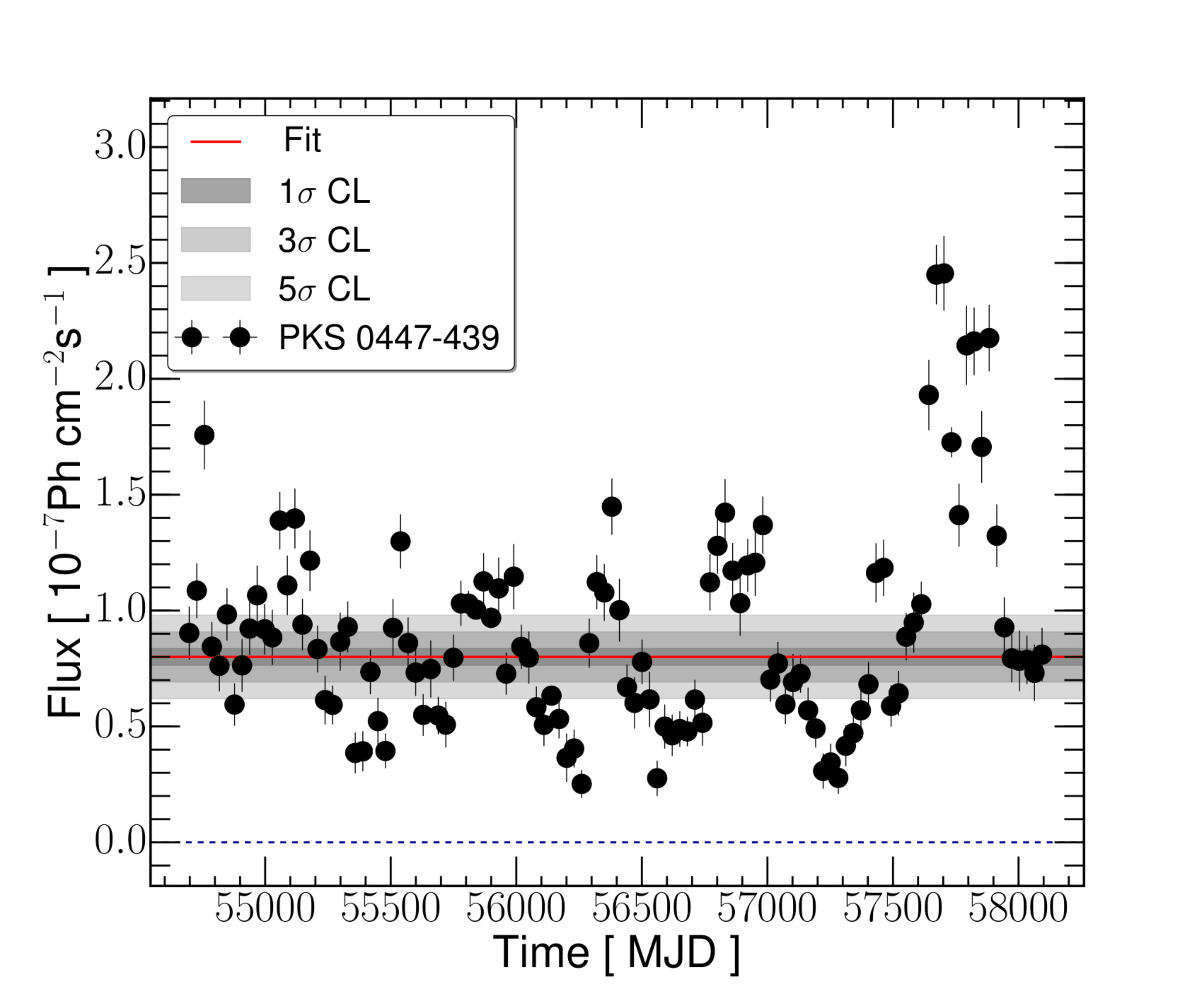 Figure 8
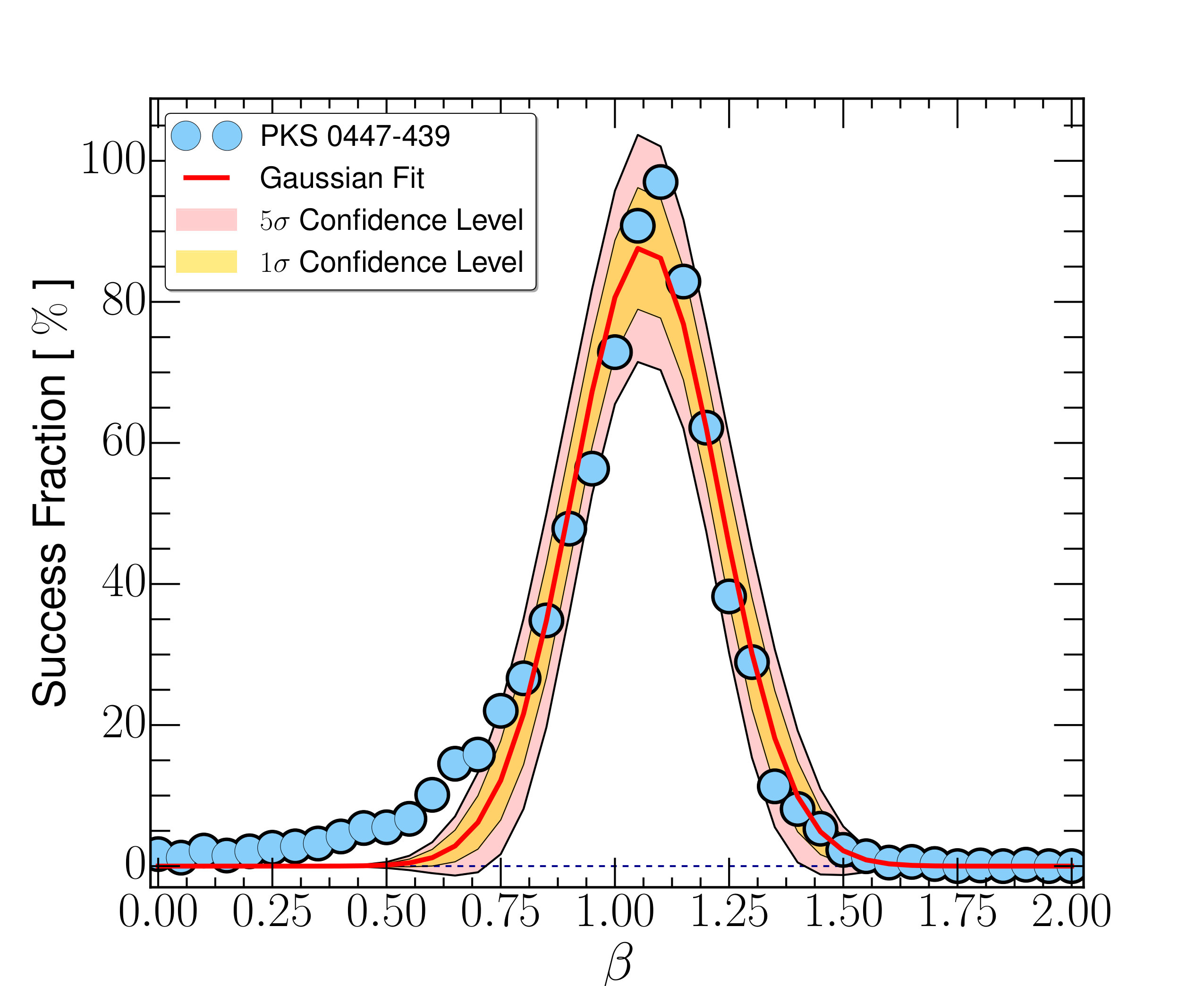 Figure 9
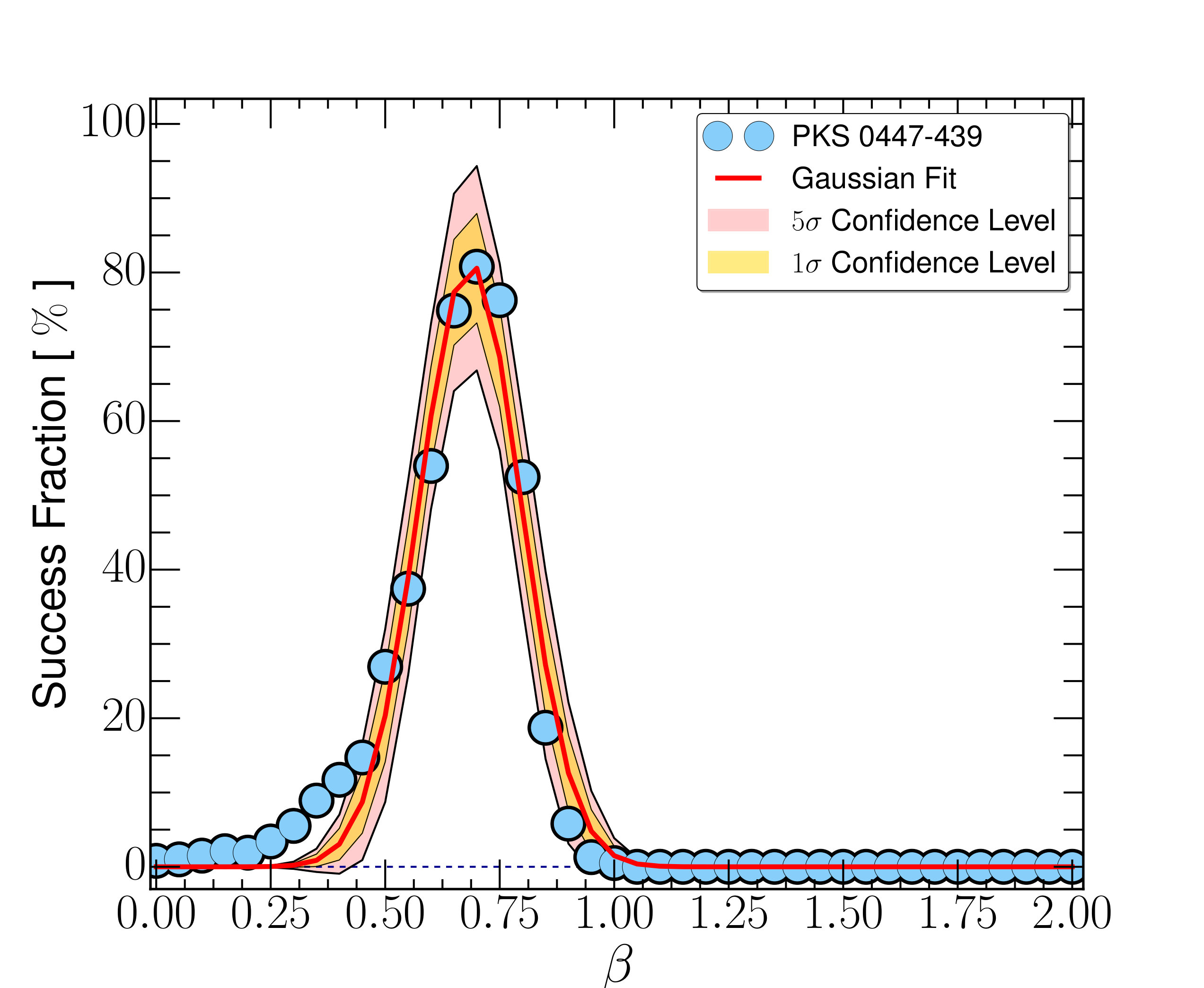 Figure 10
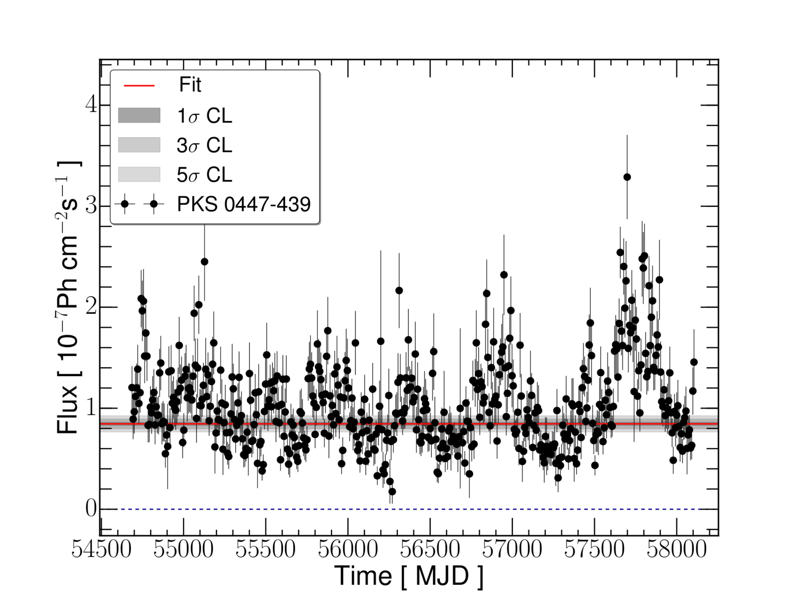 Figure 11
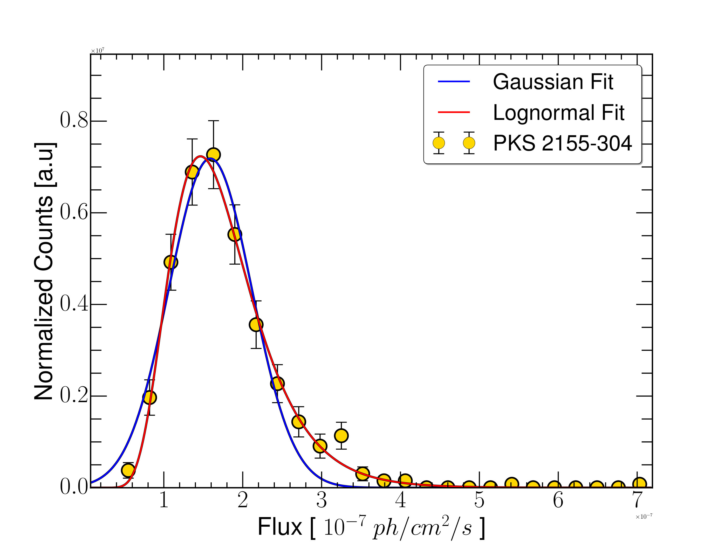 Figure 12
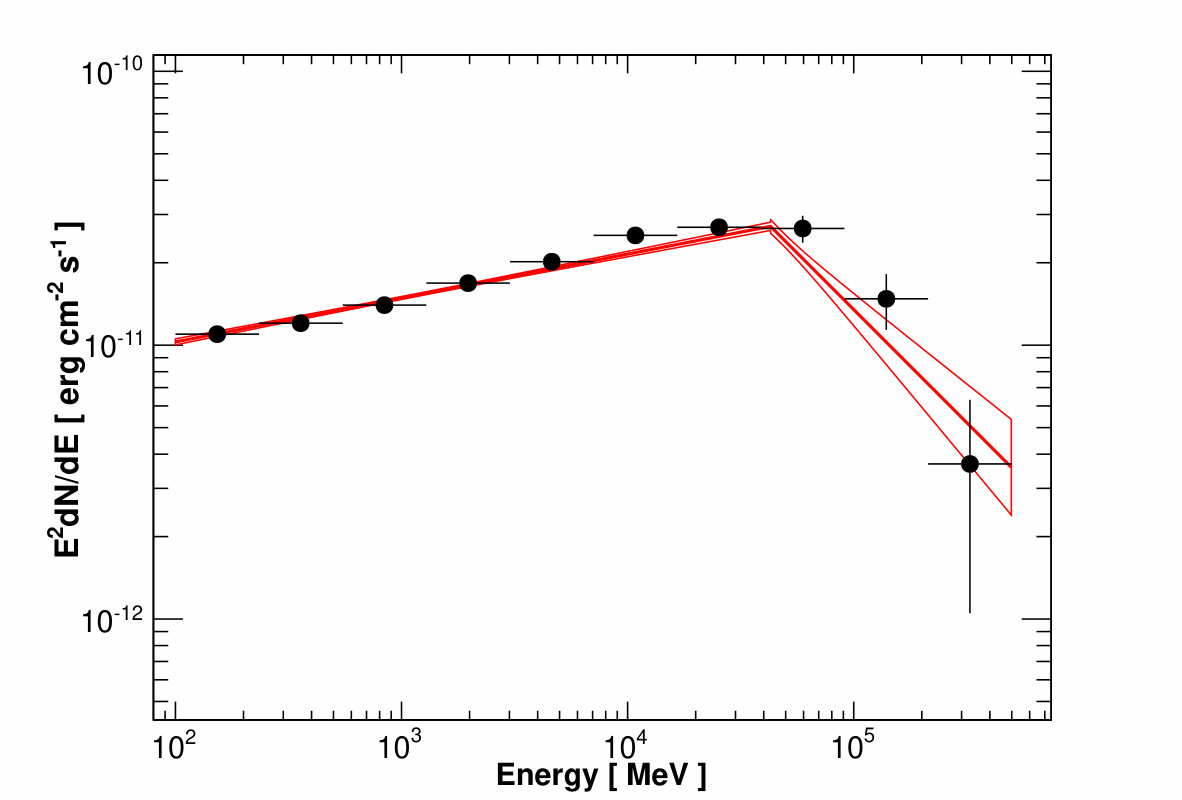 Figure 13
| Model | Energy | Spectral Parameters | Npred. | Integral Flux | TS | Log- | Log-Likelihood |
| [GeV] | Likelihood | Ratio-Test | |||||
| Power Law (PL) | .. | - | |||||
| Log Parabola | .. | - | |||||
| (LP) | |||||||
| Broken PowerLaw | .. | - | |||||
| (BPL) | |||||||
| PLSuperExpCutOff | .. | - | |||||
| Source | Model | Energy | Spectral Parameters | Integral Flux | TS | Ratio- | Fvar |
|---|---|---|---|---|---|---|---|
| [GeV] | Test | [%] | |||||
| PKS 0447-439 | Broken PowerLaw | .. | |||||
| PG 1553+113 | Log Parabola | .. | |||||
| PKS 2155-304 | PLSuperExpCutOff | .. | |||||
| PKS 0426-380 | Log Parabola | .. | |||||
| PKS 0301-243 | Log Parabola | .. | |||||
| PKS 0537-441 | PLSuperExpCutOff | .. | |||||
| Source | Log-normal | Gaussian | ||||||
|---|---|---|---|---|---|---|---|---|
| Name | Center* | Width | AD Test | Center* | Width | AD Test | ||
| [ ] | [ ] | statistics | [ ] | [ ] | statistics | |||
| PG 1553+113 | ||||||||
| PKS 0447-439 | ||||||||
| PKS 2155-304 | ||||||||
| PKS 0426-380 | ||||||||
| PKS 0301-243 | ||||||||
| PKS 0537-441 | ||||||||
| Source | K2 | Pvalue | Shapi.- | Pvalue |
|---|---|---|---|---|
| Stati. | ( Prob.) | Wilk | (Prob.) | |
| PG 1553+113 | ||||
| PKS 0447-439 | ||||
| PKS 2155-304 | ||||
| PKS 0426-380 | ||||
| PKS 0301-243 | ||||
| PKS 0537-441 |
| Source | Energy | Redshift | Observed Period | Intrinsic Period | ||
|---|---|---|---|---|---|---|
| [ GeV ] | Monthly bins* | Weekly bins* | Monthly bins* | Weekly bins* | ||
| PG 1553+113 | .. | () | () | () | () | |
| PKS 0447-439 | .. | () | () | () | () | |
| PKS 2155-304 | .. | () | () | () | () | |
| PKS 0426-380 | .. | () | () | () | () | |
| PKS 0301-243 | .. | () | () | () | () | |
| Source Name | Observed Period | Intrinsic Period | |
|---|---|---|---|
| [ days ] | [ days ] | ||
| PG 1553+113 | |||
| PKS 0447-439 | |||
| PKS 2155-304 | |||
| PKS 0426-380 | |||
| PKS 0301-243 |
| Source | Simulation Method | Monthly | Weekly | |||
| PSRESP | Simulation | PSD-Slope | Success Fraction | PSD-Slope | Success Fraction | |
| Model | Algorithm | [ % ] | [ % ] | |||
| PG 1553+113 | Power Law | Timmer & Koenig | ||||
| Power Law | Emmanoulopoulos | |||||
| PKS 0447-439 | Power Law | Timmer & Koenig | ||||
| Power Law | Emmanoulopoulos | |||||
| PKS 2155-304 | Power Law | Timmer & Koenig | ||||
| Power Law | Emmanoulopoulos | |||||
| PKS 0426-380 | Power Law | Timmer & Koenig | ||||
| Power Law | Emmanoulopoulos | |||||
| PKS 0301-243 | Power Law | Timmer & Koenig | ||||
| Power Law | Emmanoulopoulos | |||||
| Source | Simulation | Monthly | Weekly | ||||
|---|---|---|---|---|---|---|---|
| Algorithm | PSD-Slope | local | global | PSD-Slope | local | global | |
| Significance | Significance | Significance | Significance | ||||
| PG 1553+113 | Timmer & Koenig | ||||||
| Emmanoulopoulos | |||||||
| PKS 0447-439 | Timmer & Koenig | ||||||
| Emmanoulopoulos | |||||||
| PKS 2155-304 | Timmer & Koenig | ||||||
| Emmanoulopoulos | |||||||
| PKS 0426-380 | Timmer & Koenig | ||||||
| Emmanoulopoulos | |||||||
| PKS 0301-243 | Timmer & Koenig | ||||||
| Emmanoulopoulos | |||||||
| Source | Simulation | Monthly | Weekly | ||||
|---|---|---|---|---|---|---|---|
| Algorithm | PSD-Slope | local | global | PSD-Slope | local | global | |
| Significance | Significance | Significance | Significance | ||||
| PG 1553+113 | Timmer & Koenig | ||||||
| Emmanoulopoulos | |||||||
| PKS 0447-439 | Timmer & Koenig | ||||||
| Emmanoulopoulos | |||||||
Peer Reviews
No public reviews on file for this paper yet. If you reviewed it on a platform where reviews are public (OpenReview, ICLR, NeurIPS, ICML), you can paste yours below so the community can read it here.
Videos
No videos yet. Explain this paper in a talk, walkthrough, or lecture? Add one.
11institutetext: 1 Max-Planck-Institut für Kernphysik, Saupfercheckweg 1, 69117 Heidelberg, Germany
2 ZAH, Institut für Theoretische Astrophysik, Universität Heidelberg, Philosophenweg 12, 69120 Heidelberg, Germany
3 Data Assimilation Research Centre, University of Reading, Whiteknights Rd, Reading RG6 6BB, United Kingdom
Evaluating Quasi-Periodic Variations in the -ray Lightcurves of Fermi-LAT Blazars
F. Ait Benkhali 11
W. Hofmann 11
F.M. Rieger 1122
N. Chakraborty 1133
Abstract
*Context. * The detection of periodicities in the light curves of active galactic nuclei (AGN) could have profound consequences for our understanding of the nature and radiation physics of these objects. At high energies (HE; MeV) five blazars (PG 1553+113, PKS 2155-304, PKS 0426-380, PKS 0537-441 and PKS 0301-243) have been reported to show year-like quasi-periodic variations (QPVs) with significance . As these findings are based on few cycles only, care needs to be taken to properly account for random variations which can produce intervals of seemingly periodic behaviour.
*Aims. *We present results of an updated timing analysis for six blazars (adding PKS 0447-439 to the above), utilizing suitable methods to evaluate their longterm variability properties and to search for QPVs in their light curves.
*Methods. *We generate -ray light curves covering almost ten years, study their timing properties and search for QPVs using the Lomb-Scargle Periodogram and the Wavelet Z-transform. Extended Monte Carlo simulations are used to evaluate the statistical significance.
*Results. * (1) Comparing their probability density functions (PDFs), all sources (except PG 1553+113) exhibit a clear deviation from a Gaussian distribution, but are consistent with being log-normal, suggesting that the underlying variability is of a non-linear, multiplicative nature. (2) Apart from PKS 0301-243 the power spectral density (PSD) for all investigated blazars is close to flicker noise (power-law slope ). (3) Possible QPVs with a local significance \lower 2.15277pt\hbox{;\buildrel>\over{\sim};}3\sigma are found in all light curves (apart from PKS 0426-380 and PKS 0537-441), with observed periods between yr. The evidence is strongly reduced, however, if evaluated in terms of a global significance.
*Conclusions. * Our results advise caution as to the significance of reported year-like HE QPVs in blazars. Somewhat surprisingly, the putative, redhift-corrected periods are all clustering around yr. We speculate on possible implications for QPV generation.
Key Words.:
**gamma rays : galaxies – galaxies BL Lacertae objects : individual: PKS 0447-439 – PG 1553+113 – PKS 2155-304 – PKS 0426-380 – PKS 0301-243 – PKS 0537-441 – galaxies : jets – galaxies : active – radiation mechanisms: non-thermal **
1 Introduction
Blazars belong to the most luminous and variable extragalactic sources in the Universe. They represent a special sub-class of AGN characterized by a relativistic plasma jet oriented very close to the line of sight at angles , where is the bulk Lorentz factor ( (e.g., Urry & Padovani 1995; Ackermann et al. 2015). Blazar sources are known to be variable across all wavelengths from radio frequencies to TeV -ray energies, and on a wide range of timescales from sub-minute to several years (e.g. Böttcher & Chiang 2002; Aharonian et al. 2007). Their multi-wavelength spectral energy distribution (SED) often exhibits two bumps. The first, low-energy bump (peaking at infrared to X-ray frequencies) is usually interpreted as synchrotron emission from highly relativistic electrons within in the jet. The second bump, on the other hand, peaking in the HE range has been frequently related to inverse Compton emission (IC) up-scattering of various soft photon fields (mostly synchrotron or external thermal radiation), although hadronic interactions may contribute as well.
Periodic variability in the light curves of blazars has been investigated extensively in the radio and optical band (e.g., Fan et al. 2002; Kadler et al. 2006; King et al. 2013; Bhatta et al. 2016). In this context the two prominent sources OJ 287 and 3C 279 are worth mentioning, with longterm optical periods of and years being reported, respectively (Valtonen et al. 2006; Li et al. 2009). In the high-energy gamma-ray regime only five blazars (PG 1553+113, PKS 2155-304, PKS 0301-243, PKS 0426-380 and PKS 0537-441) have been reported so far exhibiting longterm quasi-periodic variability in their -ray fluxes with significance higher than (Ackermann et al. 2015; Sandrinelli et al. 2014; Zhang et al. 2017, 2017; Sandrinelli et al. 2016; Prokhorov & Moraghan 2017). Apart from PKS 0537-441, these QPVs have been seen over the whole length of the light curve. In the majority of these cases, attempts have been made to relate the detected periodic behaviour at different wavelengths and on various timescales to the motion of two SMBHs in a binary black holes system, general helical jet structures, shocks or instabilities of the disk or jet-plasma flow (e.g., Rieger 2004; Wiita 2011; Sobacchi et al. 2017).
In the present paper we use Fermi-LAT -ray data between and to re-evaluate the five blazars mentioned above and to investigate an additional source, PKS 0449-439. Results of a periodicity search based on the generalized Lomb-Scargle periodogram (GLSP) and the Weighted Wavelet Z-transform (WWZ) are presented. The signifiance of the inferred periods is then estimated on the basis of Bootstrap resampling and light curves simulations using the Timmer Koenig as well as the Emmanoulopoulos algorithm (Timmer & Koenig 1995; Emmanoulopoulos et al. 2013)
The paper is organized as follows. Section 2 provides an exemplary illustration of the performed Fermi-LAT data analysis procedures to generate -ray light curves based on a binned likelihood method and aperture photometry technique, respectively. In Sec. 3 we describe the GLSP and WWZ technique used here to search for periodicity. Signifiance estimation and variability characterization is presented in Sec. 4. Finally, Sec. 5 provides a summary and discussion of the results.
2 Observations and Analysis
2.1 Fermi-LAT likelihood analysis
Fermi-LAT on board the Fermi satellite is a electron-positron pair-conversion -ray detector sensitive to photon in energy range between MeV and GeV. The LAT has a wide field of view of sr and observes the entire sky every 2 orbits. It has a point spread function (PSF) and the largest effective area of approximately cm2 above 1 GeV. Fermi-LAT data were downloaded from the Fermi-LAT Data Server111https://fermi.gsfc.nasa.gov/ssc/data/access/ and events were selected between August and April (MET from to ), covering about years with energy range from MeV to GeV in a circular region of interest (ROI) of degree centered on the position of each source (Atwood et al. 2013).
A binned maximum likelihood analysis (Mattox et al. 1996) is performed using the Pass 8 (P8R2) algorithms and employing the standard Fermi Science Tools v10r0p5 software package. We follow the standard procedure provided by the Fermi Science Support Center (FSSC) to reduce the data. In addition, photons coming from zenith angles larger than degree were all rejected to reduce the background from gamma rays produced in the atmosphere of the Earth (albedo) with P8R2_SOURCE_V6 instrument response functions (IRF). We performed standard quality cuts in accordance with the Pass8 data analysis criteria. The background emission was modeled using the Galactic and isotropic diffuse emission gll_iem_v06_iso and P8R2_SOURCE_V6_v06 files two. All sources from the third LAT source catalog (3FGL; (Acero et al. 2015) within the ROI are included in the model to ensure a satisfactory background modeling.
A binned-likelihood analysis with a bin size of was performed. The spectral indices were allowed to vary for sources located within a radius of around the position of the investigated source. The Test Statistic value (TS), defined as TS was used to determine the source detection significance, with threshold set to TS (). The significance of a source detection is given by (Abdo et al. 2010). In the case of PKS 0447-439 for example, the likelihood analysis reveals a point source with a high statistical significance TS corresponding to . Both energy and temporal bins with TS (or ) are set as upper limits throughout the paper.
The appearance of new sources within the ROI could in principle strongly influence the -ray spectrum and light curve of the investigated source. In order to investigate this we also searched for possible new -ray sources within a FOV of . Our analysis of year of Fermi-LAT data indicates additional transient sources beyond the 3FGL catalog; these were appropriately taken into account in the full analysis, i.e. for each additional source we sequentially add a new point source with a standard spectral definition (PowerLaw) and maximize the likelihood as a function of its flux.
We produced the -ray SED and light curves of each sources through the binned maximum likelihood fitting technique, respectively with gtlike to determine the flux and TS value for each time bin. The effect of energy dispersion below MeV is also accounted for in the analysis. For that we enabled the energy dispersion correction.
As an example, the SED of PKS 0447-439 is shown in Fig. 1 for the full time and energy range using 10 energy bins. We performed maximum likelihood analyses, exploring different spectral forms for the whole energy range, namely Single Power-Law (PL), Broken Power-Law (BPL), Log-Parabola (LP) and Power-Law Super Exponential Cutoff (PLExpCutOff). In the case of PKS 0447-439 a likelihood ratio test comparison yields TS, thus preferring BPL over PL at a significance level of . The best fit indices are and with a break at an energy GeV. The obtained results of the maximum likelihood analysis are summarized for the different models in the Table 1.
2.2 Fermi-LAT -ray light curves
We generate -ray light curves for all our six sources using the individual best fit results (i.e., a BPL model in the case of PKS 0447-439), see Table 2 for details. For comparison two methods are employed: the maximum likelihood optimization and the aperture photometry. In the analysis with the first method the -ray light curves are produced by using separate equal time-bins of one month (30 days). We apply a maximum likelihood fitting technique by running the ScienceTools gtlike to extract the flux and TS value for each time bin. In this computationally more intensive procedure, the -events are selected in a circular ROI of radius centered on the position of the source. The resulting light curve for PKS 0447-439 is shown in Fig. 2 and has an average -ray flux of cm2s*-1*. The source exhibits flux variability during the whole observational period, with flux levels of peak-to-peak oscillations changing by a factor four. The calculated fractional variability index is F (Vaughan et al. 2003; Edelson et al. 2002).
The aperture photometry method on the other hand, provides a model-independent measure of the -ray flux and is less computationally demanding. It also enables the use of short time bins whereas the maximum likelihood technique requires that time bins contain sufficient photons for the analysis. We select a very small aperture radius of to exclude most background -events and to focus on the events that are most likely associated with the source itself. We produce -ray light curves in the range between MeV and GeV using a weekly binning. The exposure of each time bin is determined with the ScienceTools gtexposure. Figure 3 shows the resultant -ray light curve for PKS 0447-439 obtained with this method.
In order to verify that the aperture photometry (AP) approach gives results which are consistent with the results obtained using the binned likelihood (BL) analysis, we performed diagnostic tests on each of the investigated blazars. The BL method is the preferred procedure for most types of Fermi-LAT analyses. Taking for granted that BL flux values are indeed more accurately measured than the AP flux, we examine the correlation between the AP and BL calculated flux to assess the performance of the AP method. This correlation is plotted for PKS 0447-439 in Fig. 4 using monthly binned light curves and the calculated value of the Pearson correlation coefficient is .
2.3 Gaussian vs Log-normal Flux Distributions
The almost continuous detection of the investigated sources over time bins of seven days provides a good opportunity to investigate whether the probability density function (PDF) for the long-term -ray emission reveals any preference for a gaussian (normal) or a log-normal flux distribution. It is expected that such a feature offers an important clue for understanding the central engine of a blazer (e.g., Uttley et al. 2005; Shah et al. 2018). A log-normal distribution of -ray fluxes, for example, would suggest that the mechanism driving the variability is multiplicative in nature rather than additive. Such multiplicative behaviour might possibly be related to accretion disk fluctuations (Lyubarskii 1997; Arévalo & Uttley 2006) or the particle acceleration process itself (Shah et al. 2018). As a possible caveat we note that PDF of stochastic processes with power spectral density (PSD) steeper than index can show deviations from normality owing to divergence of power at low frequencies (e.g., Vaughan et al. 2003).
We explore the PDF and quantify this in terms of fluxes using flux-histograms. For each source the weekly -ray fluxes were distributed in a histogram of fluxes. We fit all histograms in log-scale, with Gaussian G() and log-normal L() distribution functions given by:
[TABLE]
and
[TABLE]
respectively, where and are the standard deviation and the mean of the distribution, respectively. For illustration the obtained flux histograms for PKS 0447-439, PG 1553+113 and PKS 2155-304 are shown in Figure 5. We compute the Anderson Darling test (AD) statistics (Anderson & Darling 1954) for each of the light curves as coming from a Gaussian or a log-normal distribution. The AD allows to test the null hypothesis that a sample is drawn from a population that follows a particular distribution, e.g. in our case a normal distribution. The results obtained are shown in Table 3. The obtained (AD Test) values provide strong evidence to reject the null hypothesis of an underlying normal distribution as the AD Test statistics is greater than the relevant critical value (e.g., Stephens 1974).
Except for PG 1553+113 all sources exhibit a clear deviation from a Gaussian distribution. The flux distributions are instead compatible with being log-normal, which suggests that the underlying variability is of a non-linear, multiplicative origin. Similar results are obtained from the D’Agostino’s K2 and the Shapiro-Wilk test, see Table 3.
3 Searching for periodicity
In order to search for periodicity in blazars we apply two widely used methods, the Lomb-Scargle Periodogram and the Weighted Wavelet Z-transform to light curves.
3.1 Lomb-Scargle Periodogram
The Lomb-Scargle periodogram (LSP) is a commonly used algorithm for detecting and characterizing periodicity in unevenly sampled light curves (Lomb 1976; Scargle 1982). The standard normalized Lomb-Scargle Periodogram (LSP) is equivalent to fitting sine waves of the form , and is defined for a uneven simpled time series ( ) as
[TABLE]
The standard LSP, however, has some limitations. On the one hand, it does not take measurement errors into account; on the other hand, in the calculation the mean of the flux is subtracted, which assumes that the mean of the data and the mean of the fitted sine function are the same. To overcome those limitations we instead use the generalized LSP (GLSP) (Zechmeister & Kürster 2009). As an example the calculated GLSP for PKS 0447-439 using monthly -ray light curves (generated based on the binned likelihood) is shown in Fig. 8. A strong peak at around a period of days is apparent in this figure. We have estimated the uncertainty of the calculated period based on the half-widths at half-maxima (HWHM) of Gaussian fits to the profile at the position of the highest peak. An evaluation of confidence levels determined from Monte Carlo simulations of colored noise is explained in detail in Sec. 4.
For comparison the GLSP method has also been applied to the light curves based on aperture photometry. The possible interference of nearby sources (including background contribution) is evaluated for each source as exemplary shown in Fig. 6 and Fig. 7 for the case of PKS 0447-439. The results agree well with those obtained based on the binned likelihood method, as evident from Table 5.
The observed period Pobs. for a blazar at redshift is related to its intrinsic period by . Table 5 shows the GLSP results for all sources, except PKS 0537-441, based on both, monthly (generated based on the binned likelihood) and weekly (aperture photometry) binned light curves. Year-type HE periodicity is found for all five sources, with the results based on aperture photometry and binned likelihood method being in good agreement. For the blazar PKS 0537-441 no significant period has been found when searched for the whole light curve. Furthermore the source is estimated to have a red-noise power spectrum (Covino et al. 2019), which suggests a greater possibility of detecting a fake peak. This source has thus not been included in the following. We confirm, however, that during the initial -year high state a peak can be seen at periodicity timescale of d (see e.g., Sandrinelli et al. 2016). However, for this to be a robust result, a longer observation window showing a larger number of cycles is needed given the timescale of periodicity (Vaughan et al. 2016).
3.2 Weighted Wavelet Z-transform
The GLSP provides an excellent tool for the periodicity analysis of light curves with unevenly-spaced sampling. Nevertheless it does not account for the possibility that in some astrophysical systems quasi-periodic oscillations may develop that vary significantly in frequency and amplitude over a specified period of time. In such cases, the Weighted Wavelet Z-transform (WWZ) method turns out to be a more convenient technique for detecting and quantifying such variations (Foster 1996; Han & van der Baan 2013), and has been applied for the timing analysis of AGN light curves at different wavelengths (e.g. Bhatta et al. 2016; Mohan & Mangalam 2015). The method is based on a similar concept like LSP, where sinusoidal functions are used to fit the data; however, the waves can now be localized in both time and frequency domain to account for the possible transient nature of the QPOs (Torrence & Compo 1998; Bravo et al. 2014).
The WWZ is based on a weighed projection onto three trial functions,
[TABLE]
where the ’best-fit’ coefficients are the coefficients for which the model function best fits the data. For each projection the statistic weight is given by
[TABLE]
where is a constant that determines how rapidly the Morlet wavelet decays, and is usually chosen to be close to . The WWZ power can then be finally defined as
[TABLE]
with Vx and Vy as weighted variations of the data and the model function, respectively and Neff representing the effective number of the data points (for more details, see (Foster 1996).
The WWZ powers for PKS 0447-439 are showed in Fig. 9 as a function of both observing time (horizontal axis) and period (vertical axis). The peaks in the power characterize the strength and duration of a possible quasi-periodic modulation in the data. The WWZ indicates a characteristic period at days (around years) with peak power of about and no significant changes over time. The constancy of the period indicates that the quasi-periodicity is probably driven by a physical process that is stable over duration of observation. The results of the WWZ method are shown in Table 6. The results agree well with the GLSP results.
4 Significance and Uncertainty Estimation
The effects related to irregular sampling of a light curve and the noisy nature of the periodogram can in some situation lead to the generation of false (artificial) periods in the GLSP that could be mistaken as real periodic signal of the source. For this reason, it is important to take such effects into accounts when searching for periodicities, and to analyze their impact on GLSP carefully.
The variability of AGN light curves often exhibits a colored-noise-like behavior with power spectral density (PSD) characterized by a simple power-law of the form PSD() where is the (temporal) frequency and the power-law index.
4.1 Power Spectrum Response Method (PSRESP)
In order to determine the appropriate form of the underlying colored noise needed as an input for simulating the light curves, we first applied the Power Spectrum Response method (PSRESP; Uttley et al. (2002)), which is a widely used technique for the characterization of AGN power spectra (e.g., Chatterjee et al. 2008; Bhatta et al. 2016). The method attempts to fit the binned periodogram with different realisations of a given PSD model in order to estimate the model which maximizes the probability that observed PSD can be reproduced. Our implementation of the PSRESP method is described in full detail in Chatterjee et al. (2008). Selected details are as follow:
We consider a simple power-law model for the underlying power spectrum of the form
[TABLE]
where is the amplitude of the model at the reference frequency , correspond to the power-spectral slope and is a constant which is fixed at the Poisson noise level for the light curve. We simulate light curves starting from the underlying model and using the Timmer & Koenig algorithm (see below), and re-sample these with the same sampling interval of the observed light curves. We then calculate the periodogram of the observed light curve (P()obs.) and that of each of the simulated light curves (P()sim,i where ). The statistic is calculated from the underlying model average and observed PSD of each light curve, with
[TABLE]
where and are the minimum and maximum frequencies measured by P()obs., respectively. We calculate the for each simulated PSD P()sim,i over all frequencies between and with respect to the data. We then compare with the distribution and count the number of for which is smaller than . Finally, we calculate the success fraction m/M (goodness of fit), which gives the probabilities of a model being accepted, for a range of from to with step size of . The obtained results according to the PSRESP method are summarized in Table 7 and shown in Fig. 10
4.2 MC-simulations of colored-noise light curves
The Timmer and Koenig (TK) algorithm (Timmer & Koenig 1995) is a commonly used method to produce artificial light curves. This technique allows to generate non-deterministic (stochastic Gaussian-distributed) time series from a given underlying PSD model by randomizing both the phase and the amplitude of the Fourier components. Limitations could arise, however, for light curves that exhibit strong deviations from Gaussian distributions (e.g., a burst-like behaviour).
Given the preference for log-normality, we also simulate light curves using the method proposed by (Emmanoulopoulos et al. 2013, E13) to obtain best-fitting results from the PSRESP method. The latter E13 method is able to account for a general PDF, i.e. to match both the PSD and the probability density function (PDF) of an observed light curve, thus relaxing restrictions of the TK method. This does in fact better comply with our previous findings of non-Gaussianity in Sec. 2.3.
The results are shown in Fig. 8 using the (main value of the) best fit slope . In many cases the detected periods are close to or above . Given available data there is rather little difference between the results based on the Timmer & Koenig (1995) and the Emmanoulopoulos et al. (2013) methods. The outcome is, however, obviously dependent on the slope . Within the PSRESP inferred range quite different results can be obtained as shown in Table 9, suggesting that a narrowing-down of the PSD slope will be most relevant for assessing the real significance of the detected periods.
4.3 Statistical Confidence of GLSP-detected Period
4.3.1 Local significance
In presence of an priori expectation of periodicity either from theory or from entirely independent observations, one can compute the statistical significance of the detected period at that position. This is the so-called ”local significance” as referenced in several papers (e.g., Bell et al. 2011). Thus, in the local method, the frequency channels corresponding to the GLSP-detected period were searched and the power spectra were recorded in which the peak power at this period exceeds the observed value. Finally, the fraction of occurrences with greater power than detected period is the probability of false positive, resulting from random red noise in the observed light curve.
4.3.2 Global significance
In the majority of the cases of reported periodicities, particularly in gamma-rays, we do not have strong apriori indications of the expected periodicity. In such a circumstance, it is statistically more rigorous to evaluate the ”global” rather than the local significance (e.g. Bell et al. 2011). This constitutes computing the fraction of occurrences of larger peaks at any period within a reasonable range of timescales (dependent on the cadence properties of the light curve), relative to the detected one. This ensures that we factor in false-positives from this larger range of timescales rather than a specific period. This, so called ”look elsewhere effect” (or also Multiple Testing Problem in Statistics), can be quantified in terms of a trial factor (cf. Lyons 2008; Gross & Vitells 2010). This is defined as the ratio between the probability of detecting a peak (or period/excess) at some fixed frequency, to the probability of detecting it anywhere in the (tested) range. The ”look elsewhere effect” has been explored and factored in for detection of resonant peaks in particle physics and indeed other fields including astronomy. We therefore re-evaluated the probability that the power of any observed peak is equal to or greater than a selected value somewhere in the periodogram and calculated in this wise the global significance (cf. Vaughan 2010). The results are shown in Table. 8 and reveal that in the absence of other physical reasons for restricting the period range the QPV evidence is strongly reduced, with none of the sources reaching significance. These findings are in line with similar indications in (Covino et al. 2019).
5 Discussion and Conclusions
There are an increasing number of reports suggesting the presence of year-type periodicities in the -ray light curves of Fermi-LAT detected blazars. Given the still limited duration of the light curves (\lower 2.15277pt\hbox{;\buildrel<\over{\sim};}10 yr), care needs to be taken, however, to properly assess the significance of these periods against a colored-noise background. Vaughan et al. (2016) have shown, for example, that clear phantom periodicities can be found even in pure noise data, with typical periods corresponding to cycles over the available data.
Our systematic investigation performed in this study reveals that four out of the six investigated blazars show long-term QPO indications (local significance \lower 2.15277pt\hbox{;\buildrel>\over{\sim};}3\sigma) in their Fermi-LAT light curves with an intrinsic period around yr. As we have shown there is some uncertainty as to the significance of these periodicities. Depending on the inferred best-fit PSD slope, the (local) significance can encompass a range from to (method 1), cf. Table. 8. The QPO significance is however strongly reduced in terms of a global significance, suggesting that longterm period claims should be treated with caution.
While all sources, except PG 1553+113, show clear indications for log-normality in their distribution of fluxes, incorporation of the appropriate simulation method (Timmer & Koenig 1995 or Emmanoulopoulos et al. 2013) does not have a strong impact on the significance evaluation. Improving the PSD characterization, i.e. by narrowing down the range for the PSD slope will instead be more relevant to better assess the significance.
Though the inferred periods are only tentative, one could speculate about physical mechanisms capable of accounting for year-type periodicity. It seems in fact surprising that the intrinsic periods appear quite similar, clustering around yr for sources at different redshifts.
Perhaps one of the most natural scenarios for the origin of longterm periodic variability is related to the orbital motion in a supermassive binary black hole system (SBBHS). In principle a SBBHS phase is likely to occur in radio-loud AGN (being hosted by elliptically galaxies) at some stage. However, the periods inferred here appear rather short to plausibly relate them to orbital SBBH motion. Gravitation radiation would lead to coalescence on a characteristic timescale yr only, so that for typical systems with the presumed source state would be highly unlikely. In fact, one rather expects orbital periods of the order yr for SBBHSs in blazars (Rieger 2007). This would then also be compatible with pulsar timing constraints on the inferred gravitational background (Holgado et al. 2018). As orbital motion usually allows for the shortest periodic driving (e.g., Rieger 2004), a direct SBBH origin of the observed periods appears less likely. This does not argue against the presence of SBBHSs in blazars in general, but simply cautions to directly relate periodicities of the order of yr to such systems.
Alternatively, QPOs might be related to quasi-periodic changes in accretion flow conditions that are effectively transmitted to the jet, modulating its non-thermal emission properties. Time-dependent modulations of the transition radius between an outer cooling-dominated (standard) disc and an inner radiatively inefficient flow (ADAF), for example, could lead to periodic mass flux variations (e.g., Gracia et al. 2003). If one requires the advective timescale , with the viscosity coefficient and the gravitational radius, to be (at most) comparable to , this would place the transition radius at a characteristic scale of for a reference mass of . This seems compatible with estimates for the transition radius in BL Lacs (e.g., Cao 2003; Xie et al. 2008). This would then suggest a similar black hole mass-scale for the systems investigated here.
On the other hand, year-type QPO could perhaps also trace plasma motion in the jet close to its outer jet radius . In the lighthouse model (Camenzind & Krockenberger 1992), for example, the disk-related jet is initially rotating, leading to a helical trajectory for a component injected on scales beyond the light cylinder of the innermost part of the disk magnetosphere. Angular momentum conservation would imply a characteristic intrinsic period for such a component of yr. While collimation might occur earlier (e.g., Fendt 1997), thereby reducing the jet radius, sligthly changing footpoint radii could possibly compensate for this. The lighthouse model was originally designed to account for observed QPOs with few weeks by the taking travel time effects with respect to an outwardly moving, (single) flaring component into account. It seems likely however, that the fundamental period might be visible even if the flux would be suppressed quickly. It will be interesting to probe this with a larger source sample, as intrinsic periods in this case are expected to be less than yr for a typcial black hole mass range.
The fact that the intrinsic periods seems to be clustering around yr remains particularly interesting and suggestive of a common physical mechanism. The inferred periods are, however, only tentative. Adding one or two more cycle of data (i.e., yr) is expected to significantly improve the situation and to help to clarify their putative presence and physical implication.
Acknowledgements.
We would like to thank Stefan Wagner from Landessternwarte Heidelberg (LSW) for comments and suggestions. FMR acknowledges support by a DFG Heisenberg Fellowship RI 1187/6-1.
The reference list from the paper itself. Each links out to its DOI / PubMed record.
- 1Abdo et al. (2010) Abdo, A. A., Ackermann, M., Ajello, M., et al. 2010, Ap JS, 187, 460
- 2Acero et al. (2015) Acero, F., Ackermann, M., Ajello, M., et al. 2015, Ap JS, 218, 23
- 3Ackermann et al. (2015) Ackermann, M., Ajello, M., Atwood, W. B., et al. 2015, Ap J , 810, 14
- 4Ackermann et al. (2015) Ackermann, M. et al. 2015, Ap J , 813, L 41
- 5Aharonian et al. (2007) Aharonian, F., Akhperjanian, et al. 2007, Ap JL , 664, L 71
- 6Anderson & Darling (1954) Anderson, T. W. & Darling, D. A. 1954, Journal of the American Statistical Association, 49, 765
- 7Arévalo & Uttley (2006) Arévalo, P. & Uttley, P. 2006, MNRAS , 367, 801
- 8Atwood et al. (2013) Atwood, W. et al. 2013, Ar Xiv e-prints [ ar Xiv:1303.3514 ]