Model reduction techniques for linear constant coefficient port-Hamiltonian differential-algebraic systems
Sarah-Alexa Hauschild, Nicole Marheineke, Volker Mehrmann

TL;DR
This paper develops and adapts model reduction techniques specifically for large-scale port-Hamiltonian differential-algebraic systems, ensuring structure preservation and constraint integrity, with applications to flow and mechanical systems.
Contribution
It introduces adapted model reduction methods for port-Hamiltonian differential-algebraic systems, combining Dirac structure reduction and moment matching techniques.
Findings
Methods effectively reduce model size while preserving structure.
Validated on flow and multibody system benchmarks.
Maintains algebraic constraints during reduction.
Abstract
Port-based network modeling of multi-physics problems leads naturally to a formulation as port-Hamiltonian differential-algebraic system. In this way, the physical properties are directly encoded in the structure of the model. Since the state space dimension of such systems may be very large, in particular when the model is a space-discretized partial differential-algebraic system, in optimization and control there is a need for model reduction methods that preserve the port-Hamiltonian structure while keeping the (explicit and implicit) algebraic constraints unchanged. To combine model reduction for differential-algebraic equations with port-Hamiltonian structure preservation, we adapt two classes of techniques (reduction of the Dirac structure and moment matching) to handle port-Hamiltonian differential-algebraic equations. The performance of the methods is investigated for benchmark…
Click any figure to enlarge with its caption.
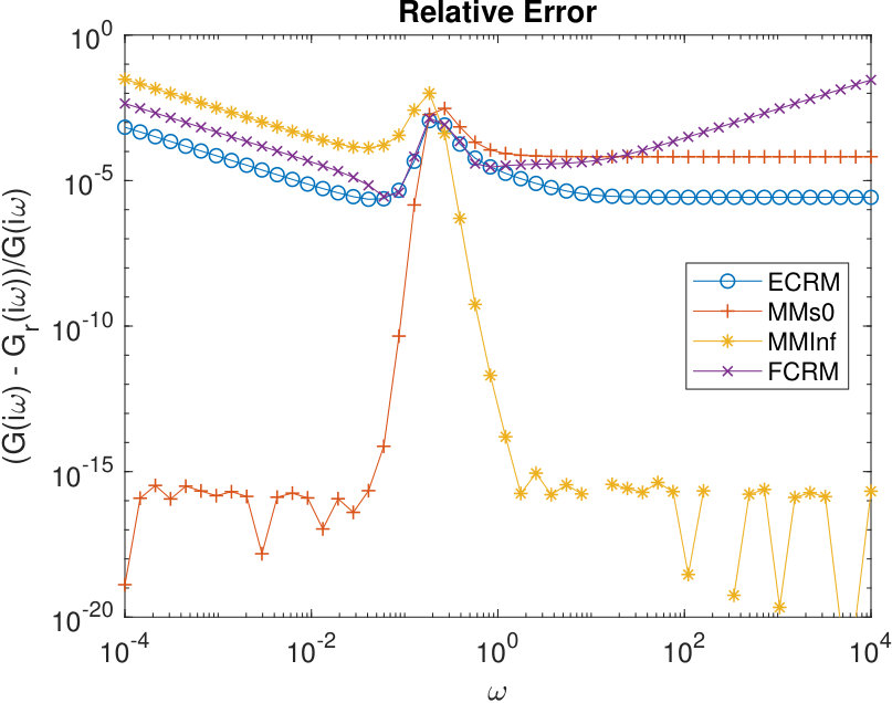 Figure 1
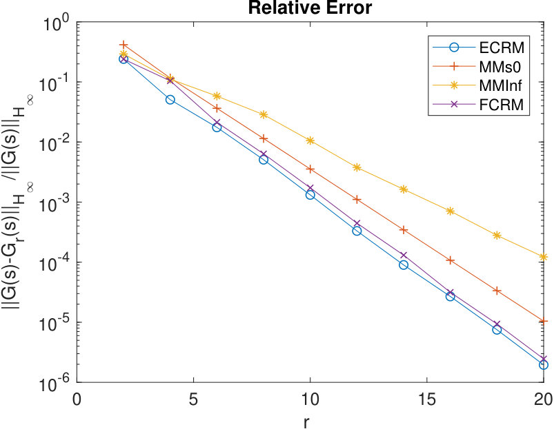 Figure 2
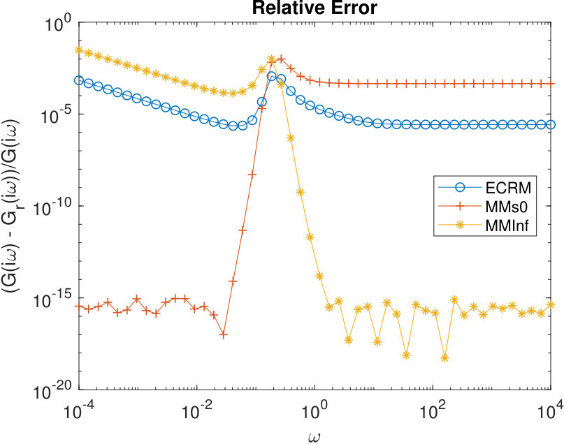 Figure 3
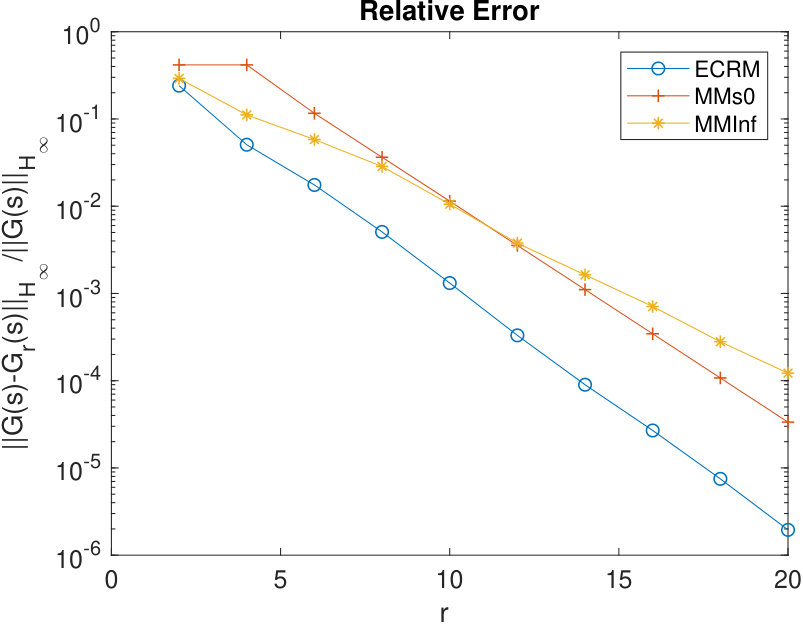 Figure 4
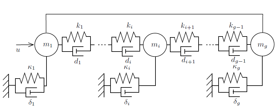 Figure 5
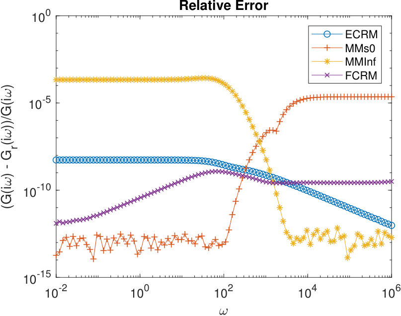 Figure 6
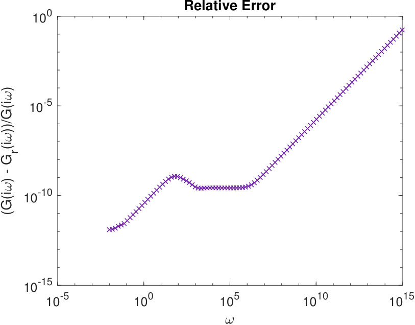 Figure 7
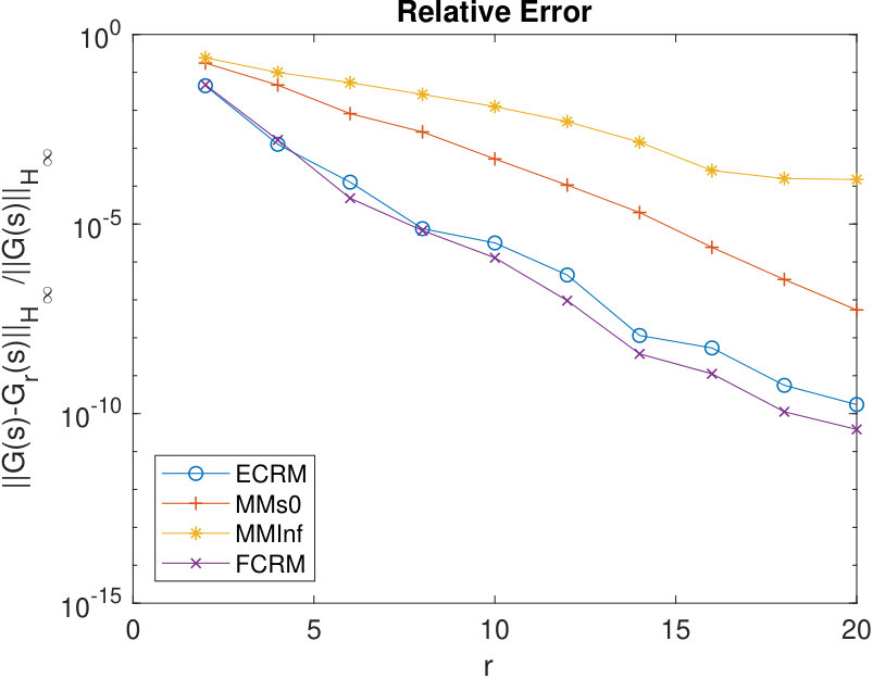 Figure 8
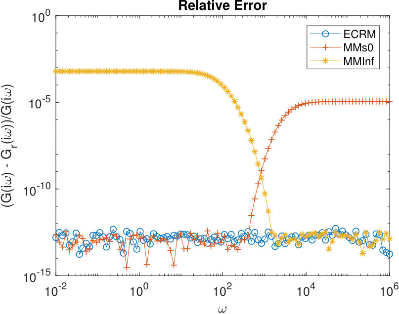 Figure 9
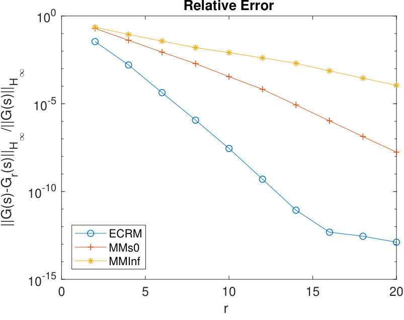 Figure 10
Peer Reviews
No public reviews on file for this paper yet. If you reviewed it on a platform where reviews are public (OpenReview, ICLR, NeurIPS, ICML), you can paste yours below so the community can read it here.
Videos
No videos yet. Explain this paper in a talk, walkthrough, or lecture? Add one.
Model reduction techniques for linear constant coefficient port-Hamiltonian differential-algebraic systems
Sarah-Alexa Hauschild1,⋆
,
Nicole Marheineke1
and
Volker Mehrmann2
(Date:
⋆ Corresponding author, email: [email protected], phone: +49 651 201 4788
1 Universität Trier, Lehrstuhl Modellierung und Numerik, Universitätsring. 15, D-54296 Trier, Germany
2 TU Berlin, Institut für Mathematik, Straße des 17. Juni 136, D-10623 Berlin, Germany )
Abstract.
Port-based network modeling of multi-physics problems leads naturally to a formulation as port-Hamiltonian differential-algebraic system. In this way, the physical properties are directly encoded in the structure of the model. Since the state space dimension of such systems may be very large, in particular when the model is a space-discretized partial differential-algebraic system, in optimization and control there is a need for model reduction methods that preserve the port-Hamiltonian structure while keeping the (explicit and implicit) algebraic constraints unchanged. To combine model reduction for differential-algebraic equations with port-Hamiltonian structure preservation, we adapt two classes of techniques (reduction of the Dirac structure and moment matching) to handle port-Hamiltonian differential-algebraic equations. The performance of the methods is investigated for benchmark examples originating from semi-discretized flow problems and mechanical multibody systems.
Keywords. structure-preserving model reduction; index reduction; port-Hamiltonian differential-algebraic system; moment matching; effort constraint method; flow constraint method
AMS-Classification. 34H05, 41A22, 65L80, 93A15, 65F22
1. Introduction
Port-Hamiltonian differential-algebraic systems (pHDAEs) arise from port-based network modeling of multi-physics problems. For this, a physical system is decomposed into smaller subsystems that are interconnected through energy exchange. The subsystems may belong to various different physical domains, such as electrical, mechanical, or hydraulic ones. The energy-based formulation is advantageous as it brings different scales on a single level, the port-Hamiltonian character is inherited by the coupling and the physical properties (e.g., stability, passivity, energy and momentum conservation) are encoded directly in the structure of the pH model equations [4, 35]. Algebraic constraints naturally come from the interconnections in form of network conditions, such as Kirchhoff’s laws, or from constraints that are directly modeled, like position or velocity constraints in mechanical systems, or from mass balances in chemical engineering problems, see e.g., [9, 23, 29]. The state space dimension of pHDAEs can be very large, e.g., for constraint finite element models in structural mechanics [17], semi-discretized problems arising in fluid dynamics [13, 14, 21, 33] or multibody problems [25]. In this case, for optimization and control, model order reduction techniques are needed that preserve the port-Hamiltonian structure and keep the explicit and hidden algebraic constraints unchanged. To present such methods and to study their properties is the main topic of this paper, which brings together model reduction for differential-algebraic equations with structure preservation.
The properties of pHDAEs have recently been studied in [4, 35]. For systems of port-Hamiltonian ordinary differential equations (pHODEs), structure-preserving reduction methods have been developed based on ideas of tangential interpolation [18, 19], moment matching [26, 27, 39] as well as effort and flow constraint reduction methods [28]. Structure-preserving model reduction for nonlinear systems has been studied in [12] and for linear damped wave equations in [13], where particular Galerkin projections have been constructed for the pHDAEs arising in gas transport networks. Surveys of model reduction techniques for general DAEs are given in [5, 7]. A crucial step for model reduction is that the dynamic and algebraic equations are exactly identified and only the dynamic equations are reduced, otherwise the system may loose important properties, such as stability or passivity.
In this paper we generalize structure-preserving techniques that have been developed for pHODEs to pHDAEs. We focus on the effort and flow constraint model reduction methods as well as on moment matching. To do this, we follow the regularization concept of [4] to identify and decouple the algebraic constraints and the dynamical equations in a structure-preserving manner to develop the corresponding reduction methods. To illustrate the performance of the reduction methods, we apply them to benchmark problems originating from semi-discretized flow calculations and multibody systems. We discuss the advantages but also the limitations of these methods for pHDAEs.
This paper is structured as follows. The model framework of port-Hamiltonian differential-algebraic systems and a structure-preserving regularization concept is presented in Section 2. Following this, structure-preserving reduction techniques for the differential-algebraic pH systems are generalized from their ordinary differential equation counterparts in Section 3. The performance of the methods is numerically investigated on the basis of various benchmark examples in Section 4. The paper closes with a summary in Section 5.
2. Model framework of port-Hamiltonian differential-algebraic systems
In this section we review the structural properties and simplified representations of pHDAEs according to [4] and [37]. In particular, we study the decoupling of the dynamic and algebraic equations and variables, that will be used in the next section to derive structure-preserving model reduction techniques.
2.1. Port-Hamiltonian systems
Port-Hamiltonian systems can be derived in two different ways, via a formulation as descriptor systems with special structured coefficient matrices or via an energy-based formulation on top of a Dirac structure. Since each formulation is a basis for a model reduction technique, we briefly discuss their relation.
Definition 1** (pHDAE).**
A linear constant coefficient DAE system of the form
[TABLE]
with , , , , , , , , on a compact interval is called a port-Hamiltonian differential-algebraic system (pHDAE) if the following properties are satisfied.
- (1)
The differential-algebraic operator
[TABLE]
is skew-adjoint, i.e., we have that and , 2. (2)
the product is positive semidefinite, i.e., , and 3. (3)
the passivity matrix
[TABLE]
is symmetric positive semi-definite, i.e., .
The quadratic Hamiltonian function of the system is given by
[TABLE]
Theorem 1**.**
Consider a pHDAE of the form (2.1). If for given input function the system has a (classical) solution in , then
[TABLE]
Furthermore, if , then .
Theorem 1 implies some important properties of a pHDAE. First of all, its Hamiltonian is an energy storage function, and the system is passive. A pHDAE satisfies a dissipation inequality. Furthermore, it is implicitly Lyapunov stable as defines a Lyapunov function. The physical properties are encoded in the algebraic structure of the coefficient matrices and the geometric structures associated with the flow of the system. In this sense, is the energy matrix, is the dissipation matrix, the structure matrix describing the energy flux among the energy storage elements, are the port matrices for energy in- and output, and , are the matrices associated to a direct feed-through from input to output . In the case that is the identity matrix, the pHDAE reduces to a standard pHODE as studied in [36].
In the alternative energy-based formulation a port-Hamiltonian system is characterized by the fact that the flow and effort variables of its energy-storing port, its energy-dissipating port and its external port are linked together in a power-conserving manner by a Dirac structure. Given a finite-dimensional linear space with its dual space , a Dirac structure is a subset satisfying for all and . For a pHDAE in the form (2.1), the flow and effort variables are defined on and , respectively. They are given by
[TABLE]
The variables of the energy-storing port are related to the evolution of the state and the Hamiltonian . If , then the constitutive relations read as . The port variables of the energy-dissipating elements satisfy a resistive relation, for all , which is encoded in the stated positive semidefinite matrix . The external port variables correspond to the out- and inputs of the system. The energy-conservation property follows directly from Theorem 1. Based on the notion of the Dirac structure, the pH system possesses a DAE representation, see [36, 37], i.e.,
[TABLE]
with matrices and where and .
2.2. Structure-preserving regularization
A pHDAE system typically contains explicit as well as implicit (hidden) constraints. Since in model reduction all constraints need to be kept unchanged in order not to destroy crucial properties, we need to identify all constraints. If the differentiation-index is larger than one, then an index reduction, e.g., via derivative arrays or minimal extension, should be performed, see [23] for general DAEs. For pHDAEs this index reduction has to be performed in a structure-preserving way, see [4]. It has been shown in [24] for the linear constant coefficient case and in [32] for the linear time-varying case that the differentiation-index will be at most two, i.e., in simple terms at most the second derivative of the input function is required to transform the system into a pHODE. In contrast to the numerical solution of pHDAEs/pHODEs via time-integration methods, which is still partially an open problem, see, e.g. [22], in the context of model reduction also a structure-preserving decoupling of the dynamic and algebraic variables should be performed. This may be a very critical step for linear time-varying or nonlinear systems, since it may require time-varying changes of variables, with all its difficulties, in particular of having to provide derivatives of the transformation functions [23]. But even in the case of constant coefficients, changes of variables with ill-conditioned transformation matrices may have to be handled.
In the following we discuss the structure-preserving regularization for linear constant coefficient pHDAEs of differentiation-index one or two. We refer to [4] for a detailed analysis of the regularization concept for linear time-varying systems. The concept is particularly based on the fact that the port-Hamiltonian structure and the associated Hamiltonian are preserved under basis change and scaling with invertible matrices (cf. Lemma 1).
Lemma 1**.**
Consider a pHDAE of the form (2.1) with Hamiltonian (2.2). Let , be invertible. Then the transformed system
[TABLE]
with , , , , , as well as and is still a pHDAE with the same Hamiltonian .
Decoupling of pHDAE of index at most one
For the decoupling of a pHDAE (2.1) of index at most one, two orthogonal matrices , are determined (e.g., via a singular decomposition) such that
[TABLE]
with invertible. We set and apply the transformation induced by and to (2.1) (cf. Lemma 1). Partitioning as in (2.4) yields block-structured system matrices whose blocks we denote by in case that they change in the decoupling procedure. As is real symmetric, we have and . Furthermore, as the system is of differentiation-index at most one, the block matrix is either not present – in case of an implicitly defined pHODE – or it is invertible, i.e., and both are invertible. Setting with
[TABLE]
and transforming (2.1) with and as in Lemma 1 yields the block-structured pHDAE
[TABLE]
where .
Theorem 2** (Decoupled pHDAE).**
Suppose that the pHDAE (2.1) is of differentiation-index at most one. Let the system be transformed to the form (2.5) via and and define . Then for any input and initial condition , the output and the state of (2.5) are given by the implicit pHODE
[TABLE]
with Hamiltonian , and coefficients
[TABLE]
The state is uniquely determined by the explicit algebraic constraint
[TABLE]
which implies a consistency constraint for the respective initial condition.
Typically the original pencil , , is regular, i.e., its determinant is not identically zero, which means that a unique solution exist for every sufficiently smooth input function and every consistent initial condition. If this is not the case, then a complex regularization procedure can be performed, which consists of transformations, feedbacks and renaming of variables, see [11]. Since this procedure is not yet available for pHDAEs, in the following we assume that is regular. Then the pencil is regular as well as shown in [24]. In this case (2.5) can be decoupled even further by identifying the zero eigenvalues of the system. For this, a change of basis is applied to the dynamic state . From it follows that the block matrix is symmetric positive semidefinite and allows for an ordered Schur decomposition that can be obtained from the generalized singular value decomposition [16]. Even though we will not carry out this transformation explicitly, it follows that the system can be transformed as
[TABLE]
Introducing yields then a pHDAE of the form
[TABLE]
Remark 1**.**
In the decoupled form (2.6), some further transformations can be applied to achieve . However, since the inverse of is involved in this transformation, we stay with the form (2.5) ((2.6), respectively).**
Decoupling for pHDAE of index two
To decouple the algebraic and differential variables for a pHDAE of differentiation-index two we make use of the index-reduction procedure developed in [4] for the linear time-varying case. Assume that the state equation with forms a DAE of index two. It has been shown in [10] that the extra constraint equations (hidden constraints) that arise from derivatives are uncontrollable, because otherwise the index reduction could have been done via feedback. This means that these hidden constraint equations are of the form . We just add these constraint equations to our original pHDAE (2.1) and obtain an overdetermined DAE system, see also [23]. Then we perform a singular value decomposition of by means of orthogonal matrices , as in (2.4) and partition the matrix associated to the extra constraints accordingly . Note that we denote blocks by in case that they change in the reduction procedure. The equations include all the constraints that are needed for index reduction. Since is invertible, these extra equations must arise from the full row-rank part of . In the following we assume w.l.o.g. that has full row-rank. This can be always achieved by transforming and omitting hidden constraint equations that do not contribute to the index reduction, see [4]. Then there exists an orthogonal matrix such that with invertible. Introducing with
[TABLE]
the hidden constraint equations become , consequently it follows that . In addition we use an orthogonal matrix such that
[TABLE]
transforming (2.1) with and as in Lemma 1 yields then the following block-structured pHDAE
[TABLE]
together with the constraint , where . Since the constraint does not change the solution, the subsystem given by the first two block rows is a pHDAE of differentiation-index at most one, i.e.,
[TABLE]
This system (2.7) can then be decoupled as described in the previous paragraph.
3. Model reduction techniques
In this section we present two different classes of model order reduction methods for pHDAEs. The first class is based on the reduction of the underlying Dirac structure and the associated power conservation, whereas the second one, the well-known moment matching, aims at the approximation of the transfer function. To derive the reduction methods, we assume that the pHDAE is in analogous form as (2.6), but for convenience we neglect the feed-through terms, i.e., we assume that and then as consequence , since . However, generalizations to systems with feed-through term are straightforward.
In the following we use an adapted notation, considering the pHDAE
[TABLE]
for the states , , with the accordingly block-structured coefficient matrices , , , and , where for , and is nonsingular.
3.1. Power conservation based model order reduction
The power conservation based methods were originally developed for standard pHODEs in [28], i.e., systems of the form (2.1) with being the identity. If for such a system a splitting of the dynamic state as exists, with and , where does not contribute much to the input-output behavior of the system, then the general idea is to cut the interconnection between the part of the energy storage port belonging to and the Dirac structure, such that no power is transferred. Then the power is exclusively exchanged via the energy storage of , which will act as reduced state variable, whereas will be skipped. The constitutive relations become
[TABLE]
with and . To cut the interconnection, one forces one of the power products or to be zero. Choosing yields the effort constraint reduction method (ECRM), while setting results in the flow constraint reduction method (FCRM).
We now adopt these reduction procedures of [28] to reduce pHDAEs in the form (2.3). Proceeding from (3), let , , , be an appropriate splitting of the dynamic part of the state variable with respect to its relevance for the input-output behavior. In the resulting system transformed by means of and as in Lemma 1 with a block diagonal matrix , we denote the state by . By definition, the flow and effort variables of the energy-storing and energy-dissipating ports inherit the partitioning, and the coefficient matrices are structured accordingly. The constitutive relations then read and , with
[TABLE]
For the model reduction we have to open the resistive port. The transformed symmetric positive semi-definite dissipation matrix admits an ordered Schur decomposition
[TABLE]
with and , with being the number of energy-dissipating elements. Plugging (3.3) into the transformed system and introducing the associated flow and effort variables accordingly, i.e., and , yields a pHDAE with opened resistive port. Inserting the constitutive relations (3.2) and introducing the external port variables , where , we obtain a new representation of (3) as
[TABLE]
In the Effort Constraint Reduction Method (ECRM) the energy transfer between the energy-storing elements and the Dirac structure is cut by setting . Here, the Hamiltonian is considered only weakly influenced by . The relation follows in a straightforward way from (3.2) as . The reduced Dirac structure is obtained by multiplying (3.4) from the left with any matrix of maximal rank satisfying , such as,
[TABLE]
Rewriting the resulting system again as DAE and closing the resistive port yields the reduced model (3).
Theorem 3** (Reduced model by ECRM).**
Consider a pHDAE of the form (3) with its representation (3.4). Then the reduced model obtained by ECRM with reduced state , is a pHDAE given by
[TABLE]
with , , where and .
Proof.
In the described reduction the port-Hamiltonian properties are inherited. The skew-symmetry of follows trivially, since
[TABLE]
The symmetry and positive semi-definiteness
[TABLE]
follows from as it is constructed from the Schur complement of a positive definite matrix. Finally,
[TABLE]
where the component is projected out by means of . ∎
In the Flow Constraint Reduction Method (FCRM), the energy transfer between the energy-storing elements and the Dirac structure is cut by setting and . Thus, is constant and can particularly be chosen as . The reduced Dirac structure is obtained by multiplying (3.4) from the left with any matrix of maximal rank satisfying , e.g., with
[TABLE]
in the case that exists. Rewriting the system as a DAE, analogously to ECRM, yields the reduced model (3.6).
Theorem 4** (Reduced model by FCRM).**
Consider a pHDAE of the form (3) with its general representation (3.4) and suppose that in (3.4) is invertible. Then the reduced order model obtained by FCRM is port-Hamiltonian and, for state , , given by
[TABLE]
with
[TABLE]
as well as with its symmetric and skew-symmetric parts, and .
Proof.
In the described reduction the port-Hamiltonian properties are inherited. It follows trivially that , are skew-symmetric and , are symmetric by construction. From it results that . Finally,
[TABLE]
holds, since is positive (semi-)definite, see [28]. ∎
The reduced models obtained by ECRM and FCRM have similarities but also show crucial differences. Obviously, , implying the same size of the reduced states. The energy matrices , only differ in the first column. In particular, ECRM generates an additive term in the matrix , and also in the matrix associated to the algebraic constraints due to the elimination of , cf. (3). Clearly, the models differ in the feed-through term which is only present in FCRM (see , and in (3.6)), even though the original system (3) did not have such a term. It is further important to note that the construction of ECRM is always applicable, whereas in the presented form FCRM requires the skew-symmetric matrix to be invertible, which is, e.g., impossible if the size is odd. In the case that is singular, the procedure has to be modified, but we do not present this modification here because it gets rather technical.
Remark 2**.**
In the presented power conservation based methods the general representation (3.4) for the pHDAE differs from the one for a standard pHODE [28] by the two additional block rows and columns for the equations associated with the kernel of the energy matrix and with the algebraic constraints. Hence, ECRM yields a reduced model (3) with equivalent block matrices in the dynamic part. However, although the reduction is only applied to the dynamic state, additional terms in associated to the algebraic constraints are generated. Also the reduced model (3.6) by FCRM contains additional blocks, i.e., , , , and , , which arise from the additional equations. The coefficients , , , , and are analogous to their counterparts for a pHODE.
3.2. Moment Matching
The model reduction procedure of moment matching (MM) derives a reduced order model by means of a Galerkin projection in such a way that the leading coefficients of the series expansion of its transfer function (its moments) match those of the full order system, i.e., with moments associated with a given shift parameter . For details of MM for DAEs we refer to [15] for and to [6] for . To apply these techniques in a structure-preserving way to the pHDAE (3), the symmetric positive definite energy matrix block associated to the dynamic state is first transformed to become an identity, as done in the works on MM for pHODEs [26, 27]. Performing a Cholesky factorization and transforming appropriately, by Lemma 1 with , , the resulting system is still port-Hamiltonian. Then a Galerkin projection matrix for the dynamic part , , can be computed, e.g., by an Arnoldi method [15], such that and its columns span a Krylov space of associated to the system shifted by [30]. Applying finally the Galerkin projection with yields the reduced model.
Theorem 5** (Reduced model by MM).**
Consider a pHDAE of the form (3) with energy matrix block . Let the projection matrix be computed by the Arnoldi method. Then the reduced system is port-Hamiltonian, matches the first moments of the full order system and is for the state , , with given by
[TABLE]
with , .
Proof.
The port-Hamiltonian structure is trivially preserved by the -associated transformation and the subsequent Galerkin projection.. The matching of the first moments is proved in [15] for and in [6] for . ∎
4. Numerical results
In this section we investigate the performance of the model reduction methods, using benchmark examples from the literature, see, e.g., [3, 8, 13, 20, 21, 25] or [33]. In order to perform model reduction, it is essential to identify all constraints arising from the physics of the problem as discussed in Section 2.2. In many applications this can be done directly by exploiting the structure of the equations coming from the physical properties.
Considering the transfer function of the original full order system, we study the approximation quality of the various reduced order systems by comparing the relative errors with being the transfer function of the reduced system. Usually this is done in the -norm in the state-space formulation or in the -norm in the frequency domain. Since the latter norm is only defined for pHDAEs of index at most one, for pHDAEs of higher index we present the errors for the index reduced system. The transfer function of a pHDAE of the form (2.1) is given by
[TABLE]
For pHDAEs of index at most one it is either a proper rational function or the sum of a proper rational function with a term that is constant in .
The numerical results have been computed with Matlab 2017a on a Linux 64-Bit machine with an Intel® Core™ i7-6700 processor. In the context of computing the error norms, see [1, 34], it is necessary to solve Lyapunov equations, for which we have used the M.M.E.S.S. Toolbox [31].
4.1. Flow problems
Consider an instationary incompressible fluid flow, prescribed in terms of velocity and pressure on the spatial domain with boundary for the time period , that is driven by external forces and dynamic viscosity . The subsequently described models of partial differential equations (Stokes as well as Oseen equations) are closed by non-slip boundary conditions and appropriate initial conditions . Spatial discretization by a finite difference method on a uniform staggered grid yield pHDAEs for the state with the semi-discretized values of the velocities and pressures , (, cf. Remark 3).
Stokes equations
A laminar flow can be modeled by the linear Stokes equations,
[TABLE]
A spatially semi-discretized differential-algebraic system for completed with an appropriate output equation is given by
[TABLE]
with the symmetric negative definite discrete Laplace operator , as well as the discrete divergence and gradient operators , . The operator usually has full row rank if the freedom in the pressure (which only occurs in differentiated form in the system) is removed, see Remark 3 on page 3. The initial conditions are and consistently . The input with input matrix results from the external forces. The output equation is supplemented accordingly regarding the port-Hamiltonian form (2.1). System (4.1) is obviously port-Hamiltonian with , and , as , and holds.
For the index reduction of the pHDAE (4.1) (which is of differentiation-index two) we do not need the whole derivative array; instead we can easily identify the equations that have to be differentiated from the special structure of the system by performing, e.g., a singular value decomposition
[TABLE]
with orthogonal matrices , and singular values , . Setting , performing an equivalence transformation with and splitting the state variable accordingly into three parts, we get the system
[TABLE]
Obviously , as the last equation is with invertible. This is the equation that has to be differentiated and inserted into the first equation to derive the second (hidden) algebraic constraint
[TABLE]
as well as a consistency condition for the initial value which relates the initial condition for and to that for . The second equation yields the underlying ODE of the system for the variable to be reduced and the output equation
[TABLE]
Note that this equation can be interpreted as the discretized heat equation in the set of divergence-free velocities [14].
In system (4.2) the skew-symmetric interconnection matrix is zero. Thus, FCRM cannot be applied directly as discussed in the previous section. Concerning ECRM, the splitting of the dynamic state is provided by Lyapunov balancing. The transformation matrices are computed by the Square-Root Algorithm [2]. Note that in this case the reduced model by ECRM is equivalent to the one obtained by using Balanced Truncation due to the symmetry of the system matrix and the relation of the input and output matrices.
Oseen equations
A flow model that is closer to the nonlinear Navier-Stokes equations is given by the Oseen equations
[TABLE]
The Oseen equations differ from the Stokes equations by the additional convective term with driving velocity . The associated spatially semi-discretized pHDAE for is given by
[TABLE]
where the appropriately discretized convective term is decomposed into its skew-symmetric part and its symmetric part. The last forms, together with the discrete Laplacian, the symmetric negative definite operator .
Analogously to the index reduction performed for the Stokes equations, we obtain as well as . The underlying ODE and the output equation are given by
[TABLE]
In system (4.3) the skew-symmetric interconnection matrix is prescribed by which, depending on the discretization scheme, may or may not be invertible. If it is invertible, then in contrast to the Stokes problem, FCRM can be applied for model order reduction. For ECRM and FCRM the balancing transformations may be computed via the Balancing Free Square-Root Algorithm [38] to preserve the structure and to avoid creating an additional energy matrix.
Remark 3**.**
In the numerical examples the flow domain is partitioned into uniform quadratic cells of edge length , . We use finite differences on a staggered grid where the velocity components are evaluated at the center of the cell faces to which they are normal and the pressure is taken at the cell centers. This procedure provides small discretization stencils and ensures numerical stability. The unknowns are
[TABLE]
for . Since the pressure is non-unique in the flow equations, we fix without loss of generality the value for the numerical solution and discard this quantity from the unknowns. The unknowns are ordered row-wise (and for the velocity component-wise) in the vectors and , where and , yielding the state , , of the pHDAE systems. **
We illustrate the model reduction techniques by comparing the approximation quality of their reduced transfer functions for both flow problems. The presented results are given for the example flow setup, where we use a random normally distributed input matrix , the dynamic viscosity and, in case of the Oseen equations, the constant convective velocity . Applying a spatial resolution of , the states have a size of for the full order pHDAE models and of for the underlying ODEs to be reduced. Figure 4.1 shows the relative errors in the spectral norm for the reduced models of size and in the -norm for . The results of MM are similar for the Stokes and Oseen equations. As expected, MM at and at yields only negligibly small errors for high or low frequencies, respectively. In the -norm MM at performs better than MM at .
For the Stokes problem the error of ECRM is small for all frequencies, oscillating around , whereas for the Oseen problem it decreases from to for increasing frequencies. In the -norm ECRM outperforms MM for both flow problems. The same error trends can be observed in the -norm. Consequently, ECRM yields better reduced models than the moment matching methods globally, as even for low and high frequencies the relative errors only differ slightly from the respective errors of MM. FCRM is not applicable to the Stokes problem and to the Oseen problem only if the invertibility requirement on the skew-symmetric interconnection submatrix is satisfied. This implies in this example setup that the size of the reduced model has to be even. Here, FCRM yields smaller errors for low frequencies than ECRM, but for higher frequencies the error increases monotonically because of the additional feed-through term in the reduced system, see also Figure 4.2. However, in the -norm FCRM even outperforms ECRM, whereas the -norm is unbounded for systems with nonzero feed-through terms.
4.2. Damped mass-spring system
The holonomically constrained damped mass-spring system is a multibody problem that describes the one-dimensional dynamics of connected mass points in terms of their positions , velocities and a Lagrange multiplier , see Figure 4.3. In the chain of mass points the th mass of weight is connected to the mass by a spring and a damper with constants and and also to the ground by a spring and a damper with the constants and , respectively, where , , , , . Furthermore, the first and the last mass points are connected by a rigid bar. The vibrations are driven by an external force (control input) acting on the first mass point. The resulting DAE system of size is not port-Hamiltonian and has differentiation-index three. In first order formulation it is given by
[TABLE]
with mass matrix , tridiagonal stiffness and damping matrices , , constraint matrix and input matrix . Assuming and to be symmetric negative semi-definite, the multibody problem can be formulated as a pHDAE of differentiation-index two by replacing the algebraic constraint by its first derivative and adding an appropriate output equation,
[TABLE]
Obviously, , , and hold. But note that is singular such that for the matrix is not invertible.
The structure of the equations simplify a further index reduction for (4.4) analogous to that for the flow problems. The singular value decomposition of , i.e., with orthogonal matrix , , as well as invertible, yields
[TABLE]
The last equation implies that . Differentiating this equation and inserting it into the second equation yields the hidden constraint for the Lagrange multiplier
[TABLE]
which also imposes a consistency condition for the initial value. The underlying ODE of size together with the output equation are given by
[TABLE]
We present numerical results for an example setup, where the parameters of the mass-spring system are set to be for and , for , as well as , and . Choosing yields a state of size for the original DAE and of for the underlying ODE to be reduced. Since the dimension is odd, the skew-symmetric interconnection matrix is singular and also the relevant submatrix for FCRM is singular as well. But MM at almost all and ECRM can be applied. Figure 4.4 shows the respective relative errors of the transfer functions in spectral norm for the reduced size and in the -norm for . As expected, MM at and yields outstanding approximations (errors of order ) for high and low frequencies, respectively. ECRM, in contrast, provides a uniformly good approximation quality of order , independently of the chosen frequency. In the - and the -norms it even outperforms the moment matching versions by one up to two orders.
Remark 4**.**
Alternatively to (4.4), the damped mass-spring system can be also formulated by keeping the original constraint and adding the additional constraint to match the symmetry structure. This is called index reduction by minimal extension, see [23], and reduces the differentiation-index to two in the system
[TABLE]
The resulting system (4.6) is of size , has a regular system matrix and a regular matrix pencil, but is not in port-Hamiltonian form. However, using again the singular value decomposition of , solving the last equation and inserting the derivative yields a pHODE for , of the form
[TABLE]
whose interconnection matrix is invertible. The other variables satisfy and . To this formulation, also FCRM and MM at are applicable. While ECRM and MM at yield analogous results independent of the problem formulation, MM at for (4.7) provides a slightly better -approximation than MM at for (4.5). FCRM shows in general a similar approximation behavior as ECRM but suffers from an error drift off for high frequencies caused by its additional feed-through terms (cf. Figure 4.4). **
5. Conclusion
The power conservation methods (ECRM and FCRM) as well as moment matching via Galerkin projections are established structure-preserving model reduction techniques for standard port-Hamiltonian systems of ordinary differential equations. In this paper we have adapted them to handle also port-Hamiltonian differential-algebraic systems of differentiation-index one or two. Making use of an appropriate decoupling of differential and algebraic variables, the dynamic state is reduced, while the properties and all explicit and hidden constraints of the pHDAE are preserved. The performance of the techniques has been illustrated for benchmark problems arising from spatially discretized flow problems and multibody systems. ECRM shows similarities to Balanced Truncation, if a Lyapunov balancing is performed. Therefore, as expected, ECRM outperforms moment matching when studying the reduction errors in - and/or -norms, whereas moment matching yields better local approximations in the spectral norm. The performance of FCRM is comparable to ECRM, but it may suffer from an error increase for high frequencies caused by the feed-through terms generated in the reduced model. Moreover, its applicability is limited.
Acknowledgements
The authors acknowledge the support by the German BMBF, Project EiFer, and the German BMWi, Project MathEnergy.
The reference list from the paper itself. Each links out to its DOI / PubMed record.
- 1[1] N. Aliyev, P. Benner, E. Mengi, P. Schwerdtner, and M. Voigt , Large-scale computation of ℒ ∞ subscript ℒ \mathcal{L}_{\infty} -norms by a greedy subspace method , SIAM Journal on Matrix Analysis and Applications, 38 (2017), pp. 1496–1516.
- 2[2] A. C. Antoulas , Approximation of Large-Scale Dynamical Systems , SIAM Publications, Philadelphia, 2005.
- 3[3] C. Beattie, S. Gugercin, and V. Mehrmann , Model reduction for large-scale dynamical systems with inhomogeneous initial conditions , Systems and Control Letters, 99 (2017), pp. 99–106.
- 4[4] C. Beattie, V. Mehrmann, H. Xu, and H. Zwart , Linear port-Hamiltonian descriptor systems , Mathematics of Control, Signals, and Systems, 30 (2018), pp. 1–27.
- 5[5] P. Benner, V. Mehrmann, and D. C. Sorensen , eds., Dimension Reduction of Large-Scale Systems , vol. 45 of Lecture Notes in Computational Science and Engineering, Springer, Berlin, 2005.
- 6[6] P. Benner and V. I. Sokolov , Partial realization of descriptor systems , Systems and Control Letters, 55 (2006), pp. 929–938.
- 7[7] P. Benner and T. Stykel , Model order reduction for differential-algebraic equations: A survey , in Surveys in Differential-Algebraic Equations. IV, Springer, Heidelberg, 2017, pp. 107–160.
- 8[8] J. Borggaard and S. Gugercin , Model reduction for DA Es with an application to flow control , in Active Flow and Combustion Control 2014, Springer, Cham, 2015, pp. 381–396.