An efficient ADER discontinuous Galerkin scheme for directly solving Hamilton-Jacobi equation
Junming Duan, Huazhong Tang

TL;DR
This paper introduces an efficient one-stage ADER discontinuous Galerkin scheme for directly solving Hamilton-Jacobi equations, achieving high order accuracy in space and time with improved computational efficiency over traditional multi-stage methods.
Contribution
The paper develops a novel ADER-DG scheme using a local spacetime Galerkin predictor, eliminating the need for multi-stage time discretization in Hamilton-Jacobi equations.
Findings
Achieves high order accuracy in space and time.
Demonstrates improved computational efficiency.
Provides explicit formulas for third-order scheme.
Abstract
This paper proposes an efficient ADER (Arbitrary DERivatives in space and time) discontinuous Galerkin (DG) scheme to directly solve the Hamilton-Jacobi equation. Unlike multi-stage Runge-Kutta methods used in the Runge-Kutta DG (RKDG) schemes, the ADER scheme is one-stage in time discretization, which is desirable in many applications. The ADER scheme used here relies on a local continuous spacetime Galerkin predictor instead of the usual Cauchy-Kovalewski procedure to achieve high order accuracy both in space and time. In such predictor step, a local Cauchy problem in each cell is solved based on a weak formulation of the original equations in spacetime. The resulting spacetime representation of the numerical solution provides the temporal accuracy that matches the spatial accuracy of the underlying DG solution. The scheme is formulated in the modal space and the volume integral and…
Click any figure to enlarge with its caption.
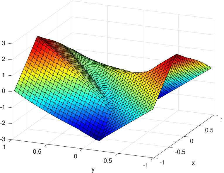 Figure 1
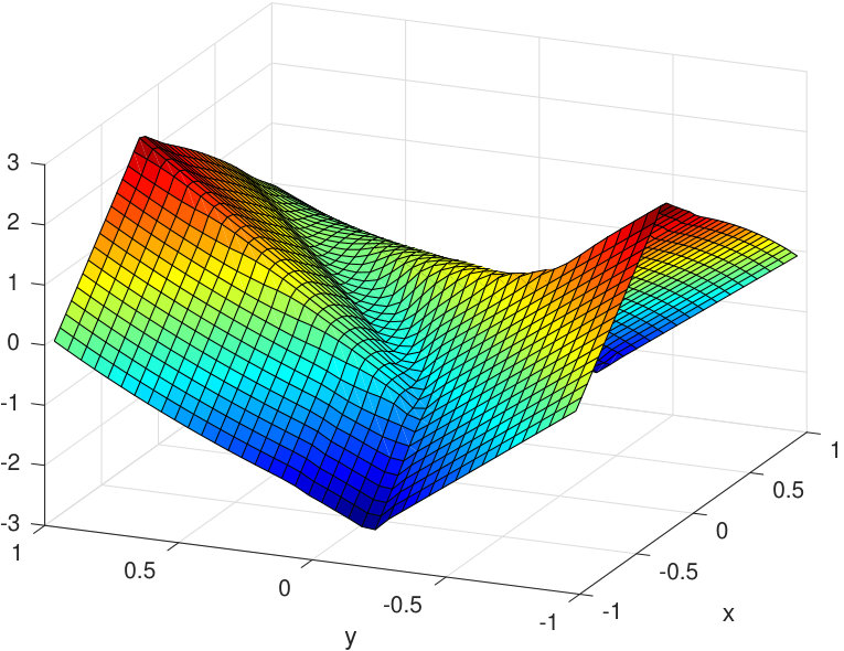 Figure 2
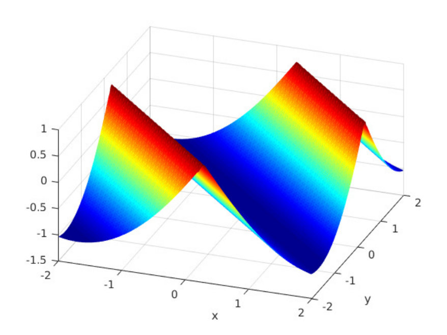 Figure 3
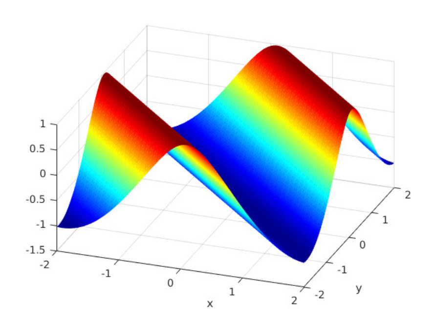 Figure 4
 Figure 5
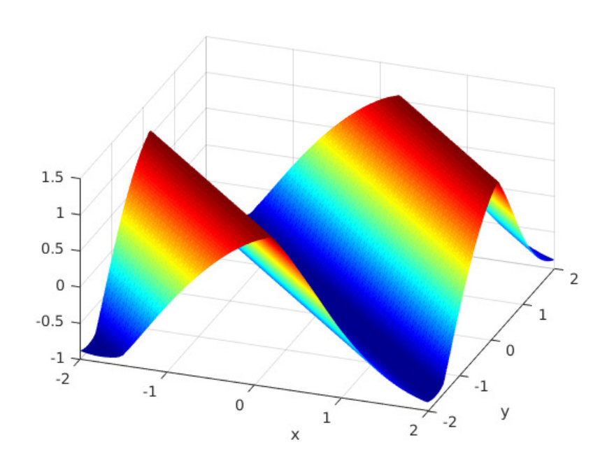 Figure 6
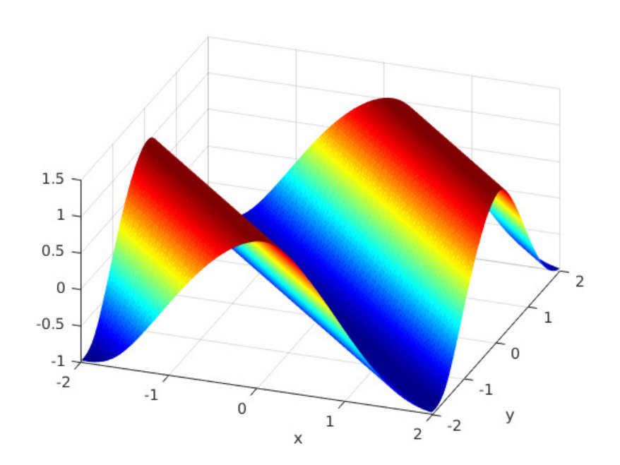 Figure 7
 Figure 8
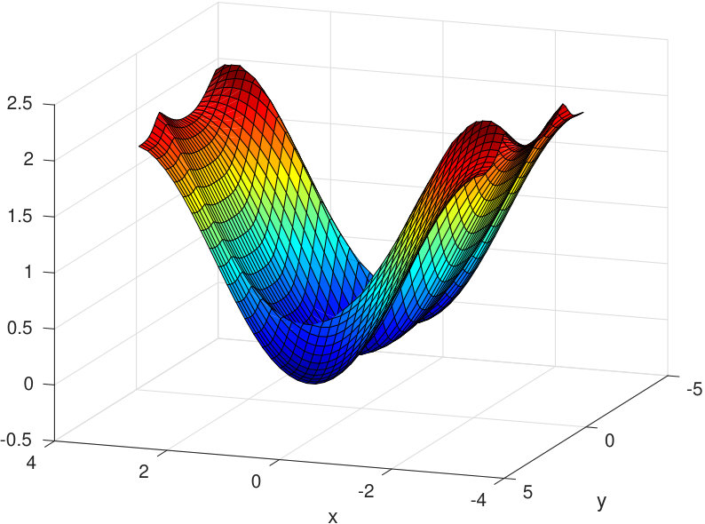 Figure 9
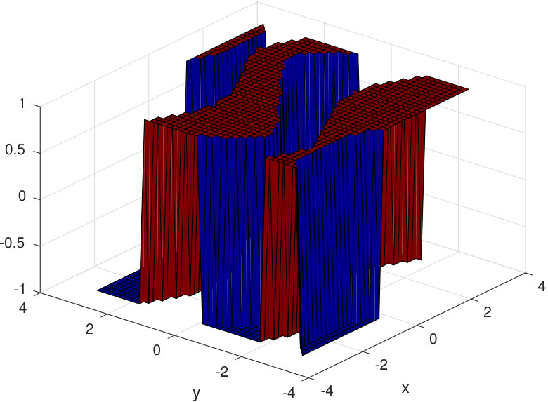 Figure 10
 Figure 11
 Figure 12
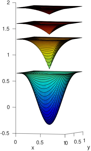 Figure 13
 Figure 14
 Figure 15
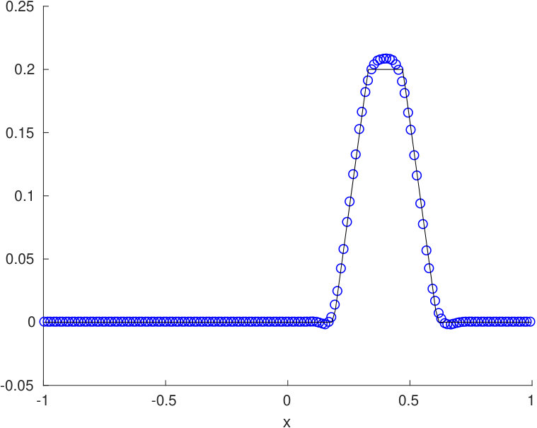 Figure 16
 Figure 17
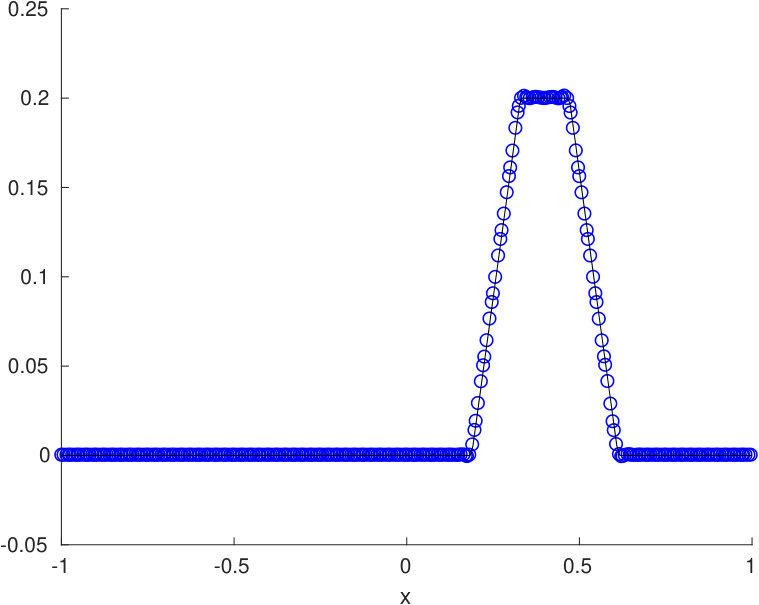 Figure 18
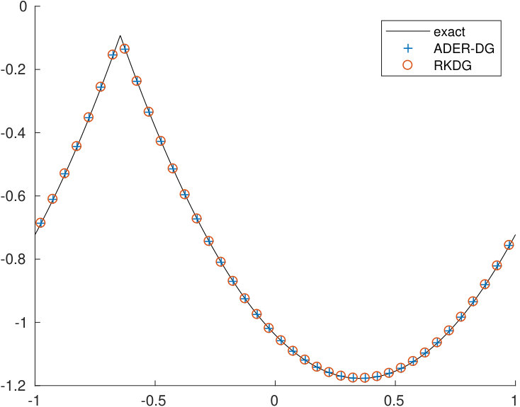 Figure 19
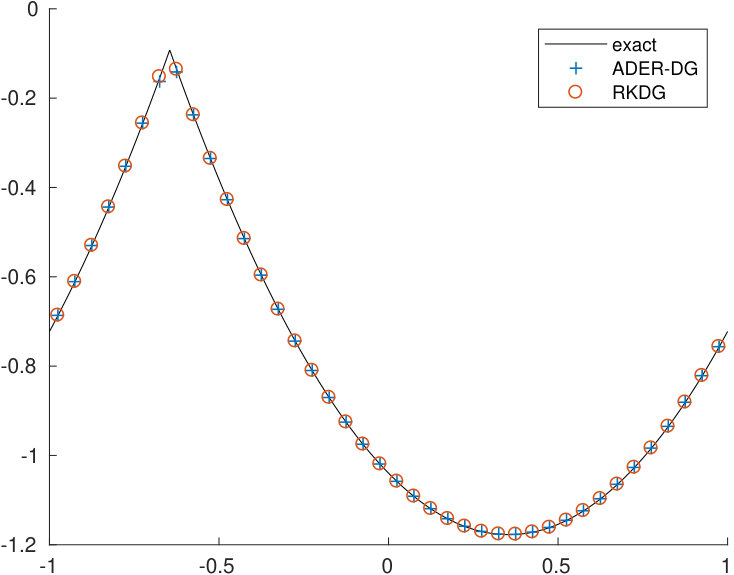 Figure 20
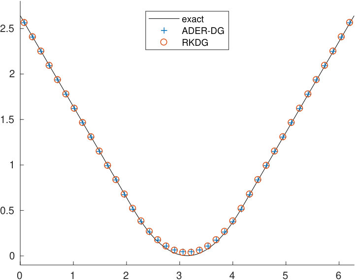 Figure 21
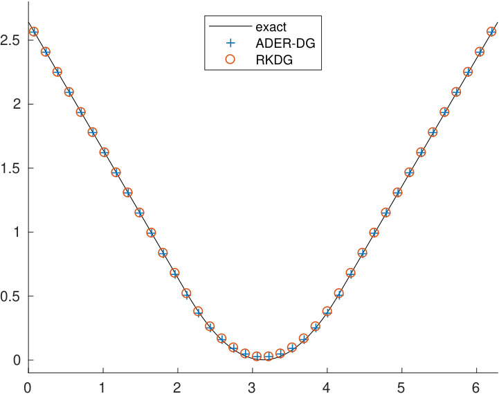 Figure 22
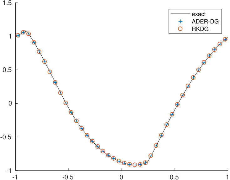 Figure 23
 Figure 24
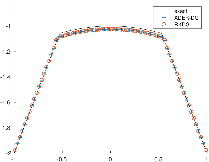 Figure 25
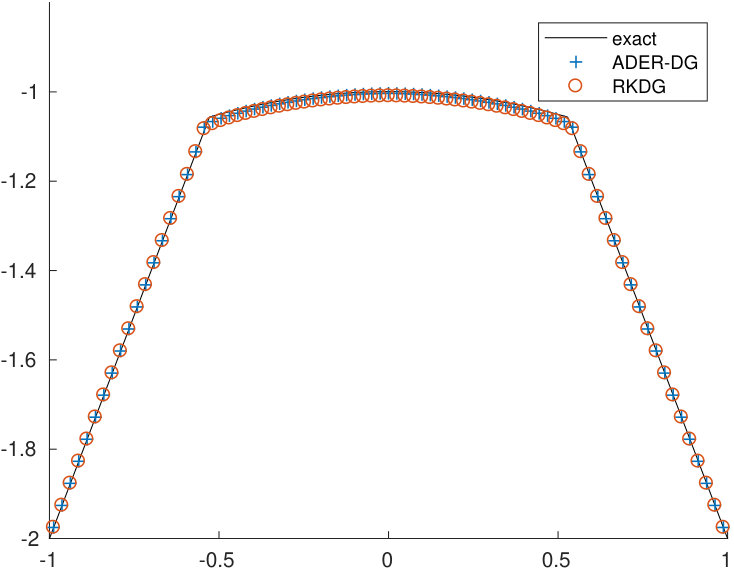 Figure 26
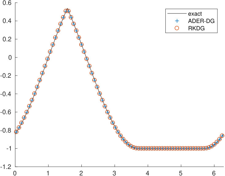 Figure 27
 Figure 28
| error | Order | error | Order | error | Order | |
| 20 | 1.322e-02 | - | 1.884e-02 | - | 1.966e-02 | - |
| 40 | 3.620e-03 | 1.87 | 5.096e-03 | 1.89 | 5.318e-03 | 1.89 |
| 80 | 9.576e-04 | 1.92 | 1.392e-03 | 1.87 | 1.524e-03 | 1.80 |
| 160 | 2.437e-04 | 1.97 | 3.458e-04 | 2.01 | 3.891e-04 | 1.97 |
| 320 | 6.157e-05 | 1.98 | 8.612e-05 | 2.01 | 9.859e-05 | 1.98 |
| 640 | 1.536e-05 | 2.00 | 2.162e-05 | 1.99 | 2.500e-05 | 1.98 |
| 20 | 1.060e-03 | - | 1.460e-03 | - | 1.761e-03 | - |
| 40 | 1.391e-04 | 2.93 | 2.022e-04 | 2.85 | 1.976e-04 | 3.16 |
| 80 | 2.033e-05 | 2.77 | 2.781e-05 | 2.86 | 3.556e-05 | 2.47 |
| 160 | 2.868e-06 | 2.83 | 3.778e-06 | 2.88 | 5.535e-06 | 2.68 |
| 320 | 3.927e-07 | 2.87 | 5.063e-07 | 2.90 | 7.534e-07 | 2.88 |
| 640 | 5.230e-08 | 2.91 | 6.658e-08 | 2.93 | 9.928e-08 | 2.92 |
| 20 | 7.609e-05 | - | 1.278e-04 | - | 9.354e-05 | - |
| 40 | 8.493e-06 | 3.16 | 1.034e-05 | 3.63 | 2.101e-05 | 2.15 |
| 80 | 6.436e-07 | 3.72 | 7.851e-07 | 3.72 | 1.307e-06 | 4.01 |
| 160 | 4.450e-08 | 3.85 | 5.410e-08 | 3.86 | 7.630e-08 | 4.10 |
| 320 | 2.939e-09 | 3.92 | 3.557e-09 | 3.93 | 4.779e-09 | 4.00 |
| 640 | 1.890e-10 | 3.96 | 2.278e-10 | 3.96 | 3.141e-10 | 3.93 |
| error | Order | error | Order | error | Order | |
| 20 | 9.156e-03 | - | 1.276e-02 | - | 5.403e-03 | - |
| 40 | 2.206e-03 | 2.05 | 3.023e-03 | 2.08 | 1.515e-03 | 1.83 |
| 80 | 3.920e-04 | 2.49 | 5.679e-04 | 2.41 | 4.227e-04 | 1.84 |
| 160 | 9.269e-05 | 2.08 | 1.355e-04 | 2.07 | 5.170e-05 | 3.03 |
| 320 | 2.111e-05 | 2.13 | 3.074e-05 | 2.14 | 1.341e-05 | 1.95 |
| 640 | 5.127e-06 | 2.04 | 7.532e-06 | 2.03 | 2.425e-06 | 2.47 |
| 20 | 3.419e-04 | - | 4.731e-04 | - | 3.417e-04 | - |
| 40 | 3.845e-05 | 3.15 | 5.057e-05 | 3.23 | 4.548e-05 | 2.91 |
| 80 | 4.185e-06 | 3.20 | 5.476e-06 | 3.21 | 5.279e-06 | 3.11 |
| 160 | 4.920e-07 | 3.09 | 6.129e-07 | 3.16 | 6.623e-07 | 2.99 |
| 320 | 6.144e-08 | 3.00 | 7.668e-08 | 3.00 | 8.205e-08 | 3.01 |
| 640 | 7.703e-09 | 3.00 | 9.629e-09 | 2.99 | 1.040e-08 | 2.98 |
| 20 | 3.168e-05 | - | 2.887e-05 | - | 5.832e-05 | - |
| 40 | 2.891e-06 | 3.45 | 2.017e-06 | 3.84 | 5.459e-06 | 3.42 |
| 80 | 9.858e-08 | 4.87 | 5.897e-08 | 5.10 | 4.190e-07 | 3.70 |
| 160 | 1.298e-09 | 6.25 | 1.268e-09 | 5.54 | 3.669e-09 | 6.84 |
| 320 | 5.215e-11 | 4.64 | 6.367e-11 | 4.32 | 3.469e-11 | 6.72 |
| 640 | 3.250e-12 | 4.00 | 3.970e-12 | 4.00 | 2.209e-12 | 3.97 |
| error | Order | error | Order | error | Order | |
| 10 | 1.307e-02 | - | 1.567e-02 | - | 2.185e-02 | - |
| 20 | 4.242e-03 | 1.62 | 4.323e-03 | 1.86 | 8.331e-03 | 1.39 |
| 40 | 8.865e-04 | 2.26 | 9.420e-04 | 2.20 | 1.986e-03 | 2.07 |
| 80 | 2.007e-04 | 2.14 | 2.250e-04 | 2.07 | 5.241e-04 | 1.92 |
| 160 | 4.850e-05 | 2.05 | 5.566e-05 | 2.02 | 1.534e-04 | 1.77 |
| 320 | 1.227e-05 | 1.98 | 1.406e-05 | 1.99 | 4.123e-05 | 1.90 |
| 10 | 1.139e-03 | - | 1.244e-03 | - | 2.522e-03 | - |
| 20 | 1.426e-04 | 3.00 | 1.452e-04 | 3.10 | 3.850e-04 | 2.71 |
| 40 | 2.034e-05 | 2.81 | 2.013e-05 | 2.85 | 5.262e-05 | 2.87 |
| 80 | 2.796e-06 | 2.86 | 2.675e-06 | 2.91 | 7.144e-06 | 2.88 |
| 160 | 3.719e-07 | 2.91 | 3.469e-07 | 2.95 | 1.298e-06 | 2.46 |
| 320 | 4.843e-08 | 2.94 | 4.456e-08 | 2.96 | 1.924e-07 | 2.75 |
| 10 | 1.320e-04 | - | 1.272e-04 | - | 2.718e-04 | - |
| 20 | 9.644e-06 | 3.78 | 8.445e-06 | 3.91 | 3.740e-05 | 2.86 |
| 40 | 7.291e-07 | 3.73 | 5.760e-07 | 3.87 | 3.211e-06 | 3.54 |
| 80 | 4.937e-08 | 3.88 | 3.793e-08 | 3.92 | 2.347e-07 | 3.77 |
| 160 | 3.231e-09 | 3.93 | 2.438e-09 | 3.96 | 1.549e-08 | 3.92 |
| 320 | 2.078e-10 | 3.96 | 1.544e-10 | 3.98 | 9.509e-10 | 4.03 |
| error | Order | error | Order | error | Order | |
| 10 | 1.082e-02 | - | 1.177e-02 | - | 2.009e-02 | - |
| 20 | 3.776e-03 | 1.52 | 3.199e-03 | 1.88 | 8.995e-03 | 1.16 |
| 40 | 7.522e-04 | 2.33 | 6.459e-04 | 2.31 | 2.063e-03 | 2.12 |
| 80 | 1.449e-04 | 2.38 | 1.380e-04 | 2.23 | 4.803e-04 | 2.10 |
| 160 | 3.011e-05 | 2.27 | 2.918e-05 | 2.24 | 1.138e-04 | 2.08 |
| 320 | 6.978e-06 | 2.11 | 7.261e-06 | 2.01 | 2.174e-05 | 2.39 |
| 10 | 1.345e-03 | - | 1.526e-03 | - | 2.355e-03 | - |
| 20 | 2.141e-04 | 2.65 | 2.359e-04 | 2.69 | 4.445e-04 | 2.41 |
| 40 | 2.968e-05 | 2.85 | 2.807e-05 | 3.07 | 7.981e-05 | 2.48 |
| 80 | 4.135e-06 | 2.84 | 3.728e-06 | 2.91 | 1.283e-05 | 2.64 |
| 160 | 5.532e-07 | 2.90 | 4.891e-07 | 2.93 | 1.704e-06 | 2.91 |
| 320 | 7.138e-08 | 2.95 | 6.098e-08 | 3.00 | 2.320e-07 | 2.88 |
| 10 | 3.630e-04 | - | 3.227e-04 | - | 1.099e-03 | - |
| 20 | 1.756e-05 | 4.37 | 1.551e-05 | 4.38 | 5.326e-05 | 4.37 |
| 40 | 1.436e-06 | 3.61 | 1.247e-06 | 3.64 | 4.616e-06 | 3.53 |
| 80 | 1.076e-07 | 3.74 | 8.771e-08 | 3.83 | 4.173e-07 | 3.47 |
| 160 | 7.396e-09 | 3.86 | 5.831e-09 | 3.91 | 4.216e-08 | 3.31 |
| 320 | 4.960e-10 | 3.90 | 3.817e-10 | 3.93 | 3.411e-09 | 3.63 |
| error | Order | error | Order | error | Order | |
| 10 | 6.631e-02 | - | 2.646e-02 | - | 5.453e-01 | - |
| 20 | 4.472e-02 | 0.57 | 1.296e-02 | 1.03 | 4.730e-01 | 0.21 |
| 40 | 2.085e-02 | 1.10 | 4.872e-03 | 1.41 | 2.831e-01 | 0.74 |
| 80 | 5.349e-03 | 1.96 | 1.066e-03 | 2.19 | 9.463e-02 | 1.58 |
| 160 | 9.966e-04 | 2.42 | 1.877e-04 | 2.51 | 1.988e-02 | 2.25 |
| 10 | 4.743e-02 | - | 1.828e-02 | - | 4.470e-01 | - |
| 20 | 2.097e-02 | 1.18 | 5.772e-03 | 1.66 | 2.832e-01 | 0.66 |
| 40 | 3.030e-03 | 2.79 | 6.260e-04 | 3.20 | 5.288e-02 | 2.42 |
| 80 | 2.383e-04 | 3.67 | 4.720e-05 | 3.73 | 4.951e-03 | 3.42 |
| 160 | 2.338e-05 | 3.35 | 4.744e-06 | 3.31 | 4.190e-04 | 3.56 |
| 10 | 3.508e-02 | - | 1.222e-02 | - | 3.618e-01 | - |
| 20 | 6.505e-03 | 2.43 | 1.706e-03 | 2.84 | 7.337e-02 | 2.30 |
| 40 | 3.530e-04 | 4.20 | 7.418e-05 | 4.52 | 6.290e-03 | 3.54 |
| 80 | 1.682e-05 | 4.39 | 3.501e-06 | 4.41 | 5.178e-04 | 3.60 |
| 160 | 9.300e-07 | 4.18 | 1.958e-07 | 4.16 | 2.627e-05 | 4.30 |
| error | Order | error | Order | error | Order | |
| 10 | 3.354e-02 | - | 2.623e-02 | - | 1.176e-01 | - |
| 20 | 1.630e-02 | 1.04 | 1.198e-02 | 1.13 | 5.408e-02 | 1.12 |
| 40 | 6.029e-03 | 1.43 | 3.973e-03 | 1.59 | 2.052e-02 | 1.40 |
| 80 | 2.705e-03 | 1.16 | 1.512e-03 | 1.39 | 1.225e-02 | 0.74 |
| 160 | 1.268e-03 | 1.09 | 5.870e-04 | 1.36 | 7.223e-03 | 0.76 |
| 10 | 1.336e-02 | - | 1.082e-02 | - | 3.939e-02 | - |
| 20 | 4.216e-03 | 1.66 | 2.883e-03 | 1.91 | 1.953e-02 | 1.01 |
| 40 | 1.964e-03 | 1.10 | 1.149e-03 | 1.33 | 9.025e-03 | 1.11 |
| 80 | 8.123e-04 | 1.27 | 3.794e-04 | 1.60 | 5.138e-03 | 0.81 |
| 160 | 3.462e-04 | 1.23 | 1.243e-04 | 1.61 | 2.919e-03 | 0.82 |
| 10 | 5.797e-03 | - | 4.822e-03 | - | 2.688e-02 | - |
| 20 | 2.525e-03 | 1.20 | 1.656e-03 | 1.54 | 1.103e-02 | 1.29 |
| 40 | 9.705e-04 | 1.38 | 5.182e-04 | 1.68 | 5.527e-03 | 1.00 |
| 80 | 3.982e-04 | 1.29 | 1.643e-04 | 1.66 | 3.026e-03 | 0.87 |
| 160 | 1.639e-04 | 1.28 | 5.113e-05 | 1.68 | 1.721e-03 | 0.81 |
| error | Order | error | Order | error | Order | |
| 10 | 1.121e-01 | - | 3.599e-01 | - | 9.131e-02 | - |
| 20 | 2.855e-02 | 1.97 | 8.840e-02 | 2.03 | 2.609e-02 | 1.81 |
| 40 | 7.174e-03 | 1.99 | 2.200e-02 | 2.01 | 6.557e-03 | 1.99 |
| 80 | 1.808e-03 | 1.99 | 5.467e-03 | 2.01 | 1.800e-03 | 1.86 |
| 160 | 4.579e-04 | 1.98 | 1.361e-03 | 2.01 | 4.963e-04 | 1.86 |
| 320 | 1.160e-04 | 1.98 | 3.391e-04 | 2.00 | 1.326e-04 | 1.90 |
| 10 | 1.970e-02 | - | 5.484e-02 | - | 2.837e-02 | - |
| 20 | 2.729e-03 | 2.85 | 7.248e-03 | 2.92 | 3.011e-03 | 3.24 |
| 40 | 3.568e-04 | 2.94 | 8.996e-04 | 3.01 | 4.757e-04 | 2.66 |
| 80 | 4.662e-05 | 2.94 | 1.157e-04 | 2.96 | 6.699e-05 | 2.83 |
| 160 | 6.024e-06 | 2.95 | 1.474e-05 | 2.97 | 9.528e-06 | 2.81 |
| 320 | 7.714e-07 | 2.97 | 1.869e-06 | 2.98 | 1.296e-06 | 2.88 |
| 10 | 5.118e-03 | - | 9.484e-03 | - | 1.798e-02 | - |
| 20 | 2.893e-04 | 4.14 | 5.677e-04 | 4.06 | 8.581e-04 | 4.39 |
| 40 | 1.932e-05 | 3.90 | 3.588e-05 | 3.98 | 6.199e-05 | 3.79 |
| 80 | 1.258e-06 | 3.94 | 2.250e-06 | 4.00 | 4.992e-06 | 3.63 |
| 160 | 8.186e-08 | 3.94 | 1.420e-07 | 3.99 | 3.548e-07 | 3.81 |
| 320 | 5.299e-09 | 3.95 | 9.022e-09 | 3.98 | 2.391e-08 | 3.89 |
| error | Order | error | Order | error | Order | |
| 10 | 1.011e-01 | - | 3.371e-01 | - | 8.475e-02 | - |
| 20 | 2.649e-02 | 1.93 | 8.548e-02 | 1.98 | 2.185e-02 | 1.96 |
| 40 | 6.610e-03 | 2.00 | 2.144e-02 | 2.00 | 6.102e-03 | 1.84 |
| 80 | 1.648e-03 | 2.00 | 5.343e-03 | 2.00 | 1.630e-03 | 1.90 |
| 160 | 4.156e-04 | 1.99 | 1.335e-03 | 2.00 | 4.330e-04 | 1.91 |
| 320 | 1.030e-04 | 2.01 | 3.326e-04 | 2.00 | 1.127e-04 | 1.94 |
| 10 | 3.503e-02 | - | 1.051e-01 | - | 2.916e-02 | - |
| 20 | 4.819e-03 | 2.86 | 1.456e-02 | 2.85 | 4.849e-03 | 2.59 |
| 40 | 5.946e-04 | 3.02 | 1.740e-03 | 3.07 | 6.406e-04 | 2.92 |
| 80 | 7.574e-05 | 2.97 | 2.102e-04 | 3.05 | 9.473e-05 | 2.76 |
| 160 | 9.764e-06 | 2.96 | 2.629e-05 | 3.00 | 1.618e-05 | 2.55 |
| 320 | 1.258e-06 | 2.96 | 3.303e-06 | 2.99 | 2.377e-06 | 2.77 |
| 10 | 7.142e-03 | - | 1.732e-02 | - | 9.557e-03 | - |
| 20 | 8.431e-04 | 3.08 | 1.703e-03 | 3.35 | 1.887e-03 | 2.34 |
| 40 | 5.677e-05 | 3.89 | 1.004e-04 | 4.08 | 2.464e-04 | 2.94 |
| 80 | 3.687e-06 | 3.94 | 6.144e-06 | 4.03 | 2.008e-05 | 3.62 |
| 160 | 2.400e-07 | 3.94 | 3.785e-07 | 4.02 | 1.323e-06 | 3.92 |
| 320 | 1.541e-08 | 3.96 | 2.378e-08 | 3.99 | 8.863e-08 | 3.90 |
Peer Reviews
No public reviews on file for this paper yet. If you reviewed it on a platform where reviews are public (OpenReview, ICLR, NeurIPS, ICML), you can paste yours below so the community can read it here.
Videos
No videos yet. Explain this paper in a talk, walkthrough, or lecture? Add one.
An efficient ADER discontinuous Galerkin scheme for
directly solving Hamilton-Jacobi equation111It is an invited paper for the special issue on “The Sixth Chinese-German Workshop on Computational and Applied Mathematics”.
Junming Duan LMAM, School of Mathematical Sciences, Peking University, Beijing 100871, China
Huazhong Tang HEDPS, CAPT & LMAM, School of Mathematical Sciences, Peking University, Beijing 100871; School of Mathematics and Computational Science, Xiangtan University, Hunan Province, Xiangtan 411105, P.R. China
Abstract
This paper proposes an efficient ADER (Arbitrary DERivatives in space and time) discontinuous Galerkin (DG) scheme to directly solve the Hamilton-Jacobi equation. Unlike multi-stage Runge-Kutta methods used in the Runge-Kutta DG (RKDG) schemes, the ADER scheme is one-stage in time discretization, which is desirable in many applications. The ADER scheme used here relies on a local continuous spacetime Galerkin predictor instead of the usual Cauchy-Kovalewski procedure to achieve high order accuracy both in space and time. In such predictor step, a local Cauchy problem in each cell is solved based on a weak formulation of the original equations in spacetime. The resulting spacetime representation of the numerical solution provides the temporal accuracy that matches the spatial accuracy of the underlying DG solution. The scheme is formulated in the modal space and the volume integral and the numerical fluxes at the cell interfaces can be explicitly written. The explicit formulae of the scheme at third order is provided on two-dimensional structured meshes. The computational complexity of the ADER-DG scheme is compared to that of the RKDG scheme. Numerical experiments are also provided to demonstrate the accuracy and efficiency of our scheme.
:
6
keywords:
Hamilton-Jacobi equation, ADER, discontinuous Galerkin methods, local continuous spacetime Galerkin predictor, high order accuracy.
5M06, 35F21, 70H20.
1 Introduction
Consider the Hamilton-Jacobi (HJ) equation
[TABLE]
with suitable boundary conditions, where denotes the Hamiltonian. The HJ equations are used in many application areas, such as optimal control theory, geometrical optics, crystal growth, image processing and computer vision. The solutions of such equations are continuous but their derivatives could be discontinuous even if the initial condition is smooth. Viscosity solutions were firstly introduced and studied in [6, 7], which are the unique physically relevant solutions.
It is well known that the HJ equations are closely related to hyperbolic conservation laws, thus many successful numerical methods for the conservation laws can be adapted for solving the HJ equations. In [7], a monotone finite difference scheme was introduced and proved to be convergent to the viscosity solution. A second order finite difference essentially non-oscillatory (ENO) scheme was developed in [16], and then a higher-order weighted ENO (WENO) scheme is proposed in [14]. Tang and his collaborators [18] developed an adaptive mesh redistribution method for the HJ equations in two- and three-dimensions. Qiu et al. [17] developed the Hermite WENO (HWENO) schemes of the HJ equations. The high order finite difference WENO scheme on unstructured meshes was developed in [21], but its implementation is a bit complicated.
Alternatively, a DG method was designed in [13] to solve the HJ equations, and its reinterpretation and simplified implementation was given in [15]. Those DG methods were based on the fact that the derivatives of the solution satisfied the conservation laws. It was correct in the one-dimensional case but at risk in the multi-dimensional case because corresponding multi-dimensional conservation laws is only weakly hyperbolic in general. Later, a DG method for directly solving the HJ equations with convex Hamiltonians was proposed in [3]. It was further improved and a new DG method was derived for directly solving the general HJ equations with nonconvex Hamiltonians in [4]. This paper will construct the scheme based on the RKDG scheme in [4]. The RKDG method [5] was originally designed to solve conservation laws, which has the advantages of flexibility on complicated geometries and a compact stencil, and is easy to obtain high order accuracy.
Most of the above methods use the multi-stage Runge-Kutta time discretization, thus have the advantage of simplicity but are time-consuming because at each stage, the volume integration and the numerical fluxes at cell interfaces have to be calculated and the nonlinear limiters should be performed to suppress the numerical oscillations. Thus, in order to save the computational cost, it is desirable to use an alternative to the multi-stage Runge-Kutta method. One choice is the Lax-Wendroff type time discretization, which converts all (or partial, when approximations with certain accuracy are expected) time derivatives in a temporal Taylor expansion of the solution into spatial derivatives by repeatedly using the underlying differential equation and its differentiated forms [12]. In [12], a local-structure-preserving DG method with Lax-Wendroff type time discretization was proposed for solving the HJ equations. It is shown that such method is relatively more efficient than the RKDG method in [15]. But the Cauchy-Kowalewski procedure may become a little cumbersome when we want to construct a high order scheme. This paper will use the time discretization (named ADER) proposed in [8, 9]. The ADER scheme has been successfully applied to the (magneto) hydrodynamics and relativistic (magneto) hydrodynamics with stiff or non-stiff source terms [1, 2, 8, 9, 11]. It is based on a local spacetime Galerkin predictor step, at which a local Cauchy problem is solved in each cell, based on a weak formulation of the original partial differential equations in spacetime. Through the above procedure, the resulting spacetime representation of the numerical solution provides the temporal accuracy that matches the spatial accuracy of the underlying DG solution. The ADER scheme is a one-step one-stage time discretization, which means that the volume integration and the numerical fluxes terms at cell interfaces are only calculated once at each time step. Our ADER-DG scheme is formulated in modal space. Thanks to the spacetime representation of the numerical solution, we can write down explicit formulae of the scheme using the strategy presented in [1], and we will provide the implementation details of the scheme at third order on two-dimensional structured meshes. Our ADER-DG scheme can capture the viscosity solution accurately and efficiently, and will be validated by the analysis of the computational complexity and the numerical experiments.
The paper is organized as follows. Section 2 presents the general formulation of our one- and two-dimensional ADER-DG schemes. Section 3 introduces the local spacetime continuous Galerkin predictor, and gives a detailed description of the two-dimensional predictor step at third order. Section 4 describes the calculation of the volume integration and the numerical fluxes terms at the cell interfaces, and the computational complexity of our ADER-DG scheme will be compared to the RKDG scheme in [4]. Section 5 presents numerical experiments and the concluding remarks are given in Section 6.
2 General formulation of the ADER-DG schemes
This section will present the general formulation of the ADER-DG schemes, in which the numerical fluxes and the penalty terms adding to the numerical fluxes are firstly developed in [4].
2.1 One-dimensional ADER-DG scheme
Let us consider the one-dimensional HJ equation at first. In this case, (1) becomes
[TABLE]
Assume the computational domain is divided into cells, , , where
[TABLE]
Denote the center of and the mesh size as and respectively. Moreover, use to denote the partial derivative of the Hamiltonian with respect to .
The spatial DG approximation space is
[TABLE]
where denotes all polynomials of degree at most on . Assume the current time interval is , and the time stepsize is . Following [4], if multiplying (2) with the test function , introducing the numerical fluxes, adding penalty terms for the numerical fluxes at the interfaces of computational cells, and integrating it over the spacetime control volume , then one has
[TABLE]
where denotes the jump of function at the cell interface, the superscripts denote the right, and left limits of a function, is a positive penalty parameter chosen as in this paper, and and are the Roe speed and the parameter to identify the entropy violating cells [4]. For all , assume is a point located at the cell interface, then and are defined by
[TABLE]
It is worth noting that the above definitions only make sense for . That is why we choose the DG space as .
Calculate the time derivative parts in (4), restrict the solutions to , thus (4) becomes
[TABLE]
where an element-local spacetime predictor solution is introduced to replace the solution in the integral of the Hamiltonian and the numerical fluxes, which is a high order approximation polynomial obtained by using the local spacetime Galerkin predictor, and will be presented in detail in Section 3. At time , the DG solution is known, if we get , then the DG solution can be evolved to time as from (6).
2.2 Two-dimensional ADER-DG scheme on structured meshes
Consider the two-dimensional HJ equation
[TABLE]
and the computational domain is divided into cells. with , , , and , , . Use and to denote the partial derivatives of the Hamiltonian with respect to and respectively.
The spatial DG approximation space is
[TABLE]
where denotes all polynomials of degree at most on , . Assume the current time interval is , and the time step is . Multiplying (7) with test functions , introducing the numerical fluxes and adding penalty terms for the numerical fluxes at the cell interfaces, and then integrating it over the spacetime control volume can give
[TABLE]
For all , if assuming is a point located at the cell interface in the -direction, then the Roe speed and the parameters to identify the entropy violating cells in the scheme are given by
[TABLE]
where is the average of the tangential derivative.
Similarly, for all , if denoting as a point located at the cell interface in the -direction, then the Roe speed and the parameters are given by
[TABLE]
where .
After calculating the time derivative parts in (9) and restricting the solutions to , then (9) becomes
[TABLE]
where the element-local spacetime predictor solution will be introduced in Section 3. The remaining task is to give .
3 Local spacetime continuous Galerkin predictor
Unlike the classical ADER schemes in [19, 20] using Cauchy-Kovalewski procedure, which may become cumbersome for high order schemes, the new formulation of ADER schemes proposed in [8] is based on a local weak formulation of the governing PDE in spacetime. The new ADER schemes rely on an iterative predictor step to obtain the spacetime representation of the solution within each cell, i.e., the previous mentioned local spacetime predictor solution . This part will construct the predictor step, and give the implementation details of the predictor step in the two-dimensional case at third order.
3.1 General formulation of continuous Galerkin predictor
For the sake of convenience, we will only consider the two-dimensional case. Assume the spatial coordinates in the reference element is , and the temporal coordinates in the reference element is . In the reference element, Eq. (7) can be written as
[TABLE]
where , and are the mesh sizes of the cell. The ADER scheme used here is a modal variant of the ADER scheme with a continuous Galerkin representation in time described in [8]. Assume that there are spacetime basis functions in the reference element, . The continuous Galerkin approach requires that the first elements in the set of basis functions only depend on the space but not on time , that is to say, only depend on the space, . Now the numerical solution can be represented in the basis space as
[TABLE]
where is a vector of modes. Similarly, the Hamiltonian can also be represented in the form of (12), . The transcription from to will be given in the next subsection. Another simplification of the continuous Galerkin approach is that the solution is continuous with the initial condition at , which means we only have to calculate once at . If the initial condition can be represented in the modal space as
[TABLE]
then at , .
Applying the Galerkin approach to (11) gives
[TABLE]
where the angled brackets denote the spacetime integration over the reference element, and the Einstein summation convection is used. Eq. (14) can be rewritten in the matrix-vector form
[TABLE]
where and are the time-stiffness matrix and the mass matrix respectively, and the -th elements of them are
[TABLE]
From the previous assumption and simplification, we know that only the last elements of are needed to be determined in the continuous Galerkin predictor step. So we can split into two parts , where is the first components and is the last components. A similar split can be done for , then the mass matrix and the time-stiffness matrix can be written as
[TABLE]
where the dimensions of sub-matrices are respectively, and it is similar for the sub-matrices of . In (15), only the last components are useful, and they can be written as
[TABLE]
where . We can obtain from through one iteration using the above equation. In the continuous Galerkin predictor step, times iterations of Eq. (18) are adequate for a -th order scheme [1], thus the cost of the iterative part in our scheme is not high. Once the basis functions are determined, the matrices in (18) are known, and the whole iterative scheme can be explicitly written down. We are going to describe the implementation details in the next subsection.
3.2 Implementation details of 2D third order continuous Galerkin predictor
This subsection will give the implementation details at third order. Other cases can be completed similarly and we will provide some difference of the implementation in other cases in Remark 3.1. Assume that the basis functions in the reference element are orthogonal Legendre polynomials
[TABLE]
Thus the solution at time or can be represented as a combination of basis functions
[TABLE]
Take the basis functions in the temporal reference element as
[TABLE]
the first three of which are needed for the third order scheme while the last basis function is only needed for fourth order schemes. In order to obtain full third order accuracy in space and time we use a total of basis functions, and the continuous Galerkin predictor solution can be expressed as
[TABLE]
noticing that the first coefficients have been substituted by due to the simplification.
Now we can explicitly write down the iterative equation (18)
[TABLE]
which give one iteration in the predictor step.
At last we have to obtain from . The most accurate way is to use the projection, but it is expensive to do lots of numerical integration. Following [1], we use the nodal approach to determine . Choose points in the reference element, where is equal to or slightly larger than . In the two-dimensional case at third order, we choose nodal points
[TABLE]
Then we can define two component vectors and , which are the nodal values of and , and their ordering follows that of nodal points. Without ambiguity in the text, here we use bar to denote the values at nodal points, which are not the cell average values defined in the numerical fluxes. and can be written down explicitly
[TABLE]
also noticing that the first eight elements of and only depend on the initial condition, thus they only have to be calculated once in the predictor step. Once we obtain and , we can get the values of at each nodal points respectively, denoted by . The above formulae give a transcription from modal space to nodal space. Then we may express the transcription from nodal space to modal space explicitly, where are temporary variables to save cost in the calculation
[TABLE]
Similarly, we only have to compute the first six coefficients once, while the last four need to be determined in the iterative predictor step. So far we have provided all the implementation details of the continuous Galerkin predictor step in the two-dimensional case at third order.
Remark 3.1**.**
For the strategy to choose the points in the reference element, we refer the readers to [1]. In this paper, the points we choose in the one-dimensional case are
second order: , 2. 2.
third order: , 3. 3.
fourth order: .
The points we choose in the two-dimensional case are
second order: , 2. 2.
fourth order:
[TABLE]
Once those points are determined, the transcription between modal space and nodal space can be obtained by the similar procedure described for two-dimensional case at third order.
4 Calculation of the volume integral and the numerical fluxes in the ADER-DG scheme
In the RKDG scheme [4], we have to calculate the volume integral of Hamiltonian, and the numerical fluxes (in two-dimensional case or above) by numerical integration, so that we have to compute Roe speed and the parameter at every integration point at cell interfaces, which is expensive. If we use the same way to accomplish them in the ADER-DG scheme, the computational complexity will be much larger, because one more dimension will appear in the ADER-DG scheme. For the volume integral, thanks to the spacetime representation of the Hamiltonian in the spacetime control volume, it can be expressed explicitly. For the numerical fluxes, we use a substantially simpler strategy presented in [10] to calculate the numerical fluxes in our ADER-DG scheme.
4.1 The explicit formulae of the volume integral
Because we have saved all in each cell, i.e. the coefficients of the basis functions, and the test functions in (10) are transformed from the six basis functions in (20) to the computational cell , we can write down the spacetime integral of the Hamiltonian in the ADER-DG scheme (10) immediately
[TABLE]
4.2 The explicit formulae of the numerical fluxes
In [10], the central idea consists of freezing the wave speeds to equal their values evaluated at the spacetime barycenters of the face under consideration. For the numerical fluxes considered here, we would freeze the Roe speed and the parameter to their values at the spacetime barycenters, then the remaining parts can be explicitly calculated. Now we take the face for example, whose left neighbor cell is , and the right is . In order to calculate the Roe speed and the parameter at the spacetime barycenter , we need to give the left and right limit values of the partial derivatives at the point
[TABLE]
where the subscripts and denote values in the left and right side respectively, and denote the partial derivatives and respectively. Then we can obtain and by using the definition (28) at . Now freeze and in the numerical fluxes terms in the ADER-DG scheme (10), and introduce three temporary variables as
[TABLE]
Denote the basis functions in the left cell and in the right cell by and respectively. For the first basis function , we have
[TABLE]
and the numerical fluxes terms in (10) are
[TABLE]
where the first and the third integrations are the contributions to the left cell, and the second and the fourth integrations are the contributions to the right cell. For the second basis function transformed from and the fourth basis function transformed from , the corresponding integrations are
[TABLE]
and
[TABLE]
We can clearly see from the above formulae that, for the second and the fourth basis functions, the numerical fluxes terms are just a scaling of the corresponding numerical fluxes terms for the first basis function, thus the computational costs can be reduced greatly. Similarly, if denoting
[TABLE]
then for the third basis function transformed from and the sixth basis function transformed from , the four numerical fluxes terms in (10) corresponding to (30) are
[TABLE]
and
[TABLE]
respectively. If denoting
[TABLE]
then for the fifth basis function transformed from , the four corresponding numerical fluxes terms are
[TABLE]
We have explicitly given the volume integral and the numerical fluxes terms in the ADER-DG scheme (10) in the two-dimensional case at third order. In the next subsection, we would like to compare the computational complexity of the ADER-DG scheme to that of the RKDG scheme.
4.3 Comparison of the computational complexity between the ADER-DG scheme and the RKDG scheme
This section give a comparison of the computational complexities of the ADER-DG scheme and the RKDG scheme. As an example, we consider them in the two-dimensional case at third order, and are going to count the number of operations needed in the evolution procedure at a time step for one cell. Four types of basic operations, i.e., addition, subtraction, multiplication and division, are all treated as one operation. And we regard one calculation of the Hamiltonian as one operation. The main part is evolving the DG solutions in each cell, so the part for calculating the time step is negligible.
In the ADER-DG scheme, we need 79 operations to calculate the partial derivatives and and 31 operations to obtain the value of Hamiltonian, 120 operations to accomplish the transcription from nodal space to modal space, 57 operations to perform three iterations, 13 operations to calculate the volume integral of Hamiltonian. For each face, we need 28 operations to compute the Roe speed and the parameters, 84 operations for the numerical fluxes terms. Because there are four faces for a cell and each face is shared by two cells, the operations on the faces of one cell should be doubled. At one time step, we need 36 operations to evolve the DG solution in a cell, so 560 operations are needed to update one cell in a time step.
In the RKDG scheme, we need to use numerical integration. We use three points Gauss-Legendre integration on an edge, and nine points Gauss-Legendre integration in the tensor product form for the volume integral. Because the values of each basis functions at each integration points in the reference element will be used many times, we compute them once and save them. We need 11 and 12 operations to compute the value and the partial derivatives of respectively. Thus we need 486 operations to calculate the volume integral of Hamiltonian once in the RKDG scheme, and on each edge, 222 operations to compute the Roe speed and the parameter , 189 operations to compute the numerical fluxes. At each sub-step, we need 36 operations to evolve the DG solution, thus 1344 operations are needed in a sub-step and 4032 operations in total.
At second order, the number of the operations for the ADER-DG scheme and the RKDG scheme are 180 and 868 respectively, and at fourth order, they are 2358 and 12944 respectively.
The above analysis shows that the ADER-DG scheme has much less computational complexity when the solution is evolved in a cell at a time step, which is about of the RKDG scheme at second, third and fourth order, respectively. The reason is that the ADER-DG scheme is a one-step one-stage scheme and we use a cheap way to calculate the volume integral and the numerical fluxes terms in the ADER-DG schemes. Further, we will show that our schemes can achieve the designed order of accuracy in the numerical experiments, and the comparison of the CPU times will be also recorded to validate the efficiency of the ADER-DG scheme.
5 Numerical results
This section will provide some numerical experiments in one- and two-dimensions. In the two-dimensional experiments, we use uniform meshes with . The time stepsize is chosen as , where for one-dimensional cases and for two-dimensional cases.
5.1 One-dimensional results
Example 5.1**.**
We solve the following linear problem [3] with a smooth variable coefficient
[TABLE]
The initial condition is , and the periodic boundary condition is specified. The exact solution is . **
The numerical errors and the orders of convergence at are presented in Table 1. We can see that the ADER-DG scheme can achieve -th order accuracy for polynomials.
Example 5.2**.**
We solve the following linear problem [3]
[TABLE]
with initial condition , and periodic boundary condition. Obviously, the variable coefficient is not smooth. **
In the viscosity solution, there is a shock forming in at , and a rarefaction wave at , thus the numerical errors are only calculated in the smooth region . The errors and the orders of convergence at are presented in Table 2. From the table, we can observe that our schemes can achieve -th order accuracy for polynomials in the smooth region. The results obtained with and ADER-DG scheme and are also shown in Fig. 1. The ADER-DG scheme can converge to the viscosity solution.
Example 5.3**.**
We solve one-dimensional Burgers’ equation
[TABLE]
with smooth initial condition, initial condition , and periodic boundary condition. **
We compute the solution up to . At this time, the solution is still smooth. We provide the errors and the orders of convergence in Table 3. Our scheme can achieve the designed order of accuracy in this example. We also compute the solution up to , there will be a shock in . In Fig. 2, we show the results obtained with and ADER-DG scheme with . From the figures, we can see that the ADER-DG scheme can give good results.
Example 5.4**.**
We solve one-dimensional Burgers’ equation [4],
[TABLE]
with unsmooth initial condition, initial condition , and periodic boundary condition. **
There is a rarefaction wave formed in the derivative of the exact solution, thus the initial sharp corner at will be smeared out over time. Fig. 3 includes the and ADER-DG results with . Thanks to the penalty terms adding to the numerical fluxes, the results of the ADER-DG scheme converge to the viscosity solution correctly.
Example 5.5**.**
We solve one-dimensional HJ equation
[TABLE]
with a nonconvex Hamiltonian, initial condition , and periodic boundary condition. **
We compute the solution up to . At this time, the solution is still smooth. We list the errors and the orders of convergence in Table 4. In the table, -th order accuracy for polynomials can be observed.
Then we compute the solution up to . We plot the results of the ADER-DG scheme in Fig. 4. In the figures, the kinks in the solution are clearly resolved by our scheme.
Example 5.6**.**
We solve one-dimensional Riemann problem
[TABLE]
with a nonconvex Hamiltonian, initial condition . **
The results at of the ADER-DG scheme with and are plotted in Fig. 5. It is a benchmark problem to test a numerical scheme’s capability to capture the viscosity solution. Similar as the RKDG scheme in [4], Minmod limiter is used for the convergence to the entropy solution, and the result with odd gives smaller errors.
5.2 Two-dimensional results
Example 5.7**.**
We solve the following linear problem with smooth variable coefficient [4]
[TABLE]
with the initial condition
[TABLE]
and periodic boundary condition. The parameter is , and the computational time is . **
This problem describes a smooth solid body rotating around the origin. We list the errors and the orders of convergence in Table 5.
Example 5.8**.**
We solve the same problem as Example 5.7, but with a unsmooth initial condition
[TABLE]
where . **
The numerical results at are provided in Table 6. From the table, we can observe that the ADER-DG scheme is nearly first order, because the initial condition is unsmooth. But we can see from Fig. 6 that, high order scheme can obtain better results.
Example 5.9**.**
We solve two-dimensional Burgers’ equation
[TABLE]
with a smooth initial condition , and periodic boundary condition. **
We compute the solution until . It is smooth at this time. We give the numerical errors and the orders of convergence in Table 7. It is clearly that our scheme can achieve -th order of convergence for polynomial. We also compute the same equation until , and the discontinuous derivative has already appeared in the solution. We plot the results in Fig. 7, from which we can observe good resolutions of the ADER-DG scheme for this example.
Example 5.10**.**
We solve the following two-dimensional equation with nonconvex Hamiltonian
[TABLE]
with initial condition , and periodic boundary condition. **
The solution is still smooth at , and the numerical errors and the orders of convergence at this time are listed in Table 8. We also compute the same equation until , and singular features develop in the solution. The results of the ADER-DG scheme are shown in Fig. 8.
Example 5.11**.**
We solve the following problem from optimal control
[TABLE]
with initial condition , and periodic boundary condition. **
The results obtained by the ADER-DG scheme with and are plotted in Fig. 9. We can see that our scheme can simulate the problem well.
Example 5.12**.**
We solve the following two-dimensional Riemann problem
[TABLE]
with initial condition . **
We need limiters in this example to have its convergence to the viscosity solution. The results of and ADER-DG scheme with are given in Fig. 10. Our results are nearly the same as that in [4].
Example 5.13**.**
We solve the problem of a propagating surface, which is a special case of the example in [16]
[TABLE]
with initial condition . **
We output the results at , and plot them in Fig. 11. The result at is shifted down to show the detail of the solution at later time.
At the end of this section, presents a comparison of the CPU times of the ADER-DG and RKDG schemes when they are applied to the above three two-dimensional examples, Examples 5.7, 5.9, and 5.10. To make the fair comparison, we take the largest CFL number of both schemes, although we have to use a slightly smaller CFL number for the ADER-DG scheme in some cases. The results given in Table 9 show that the average CPU times of the ADER-DG scheme are about of the RKDG scheme at second, third and fourth order, respectively, and the ADER-DG scheme is more efficient than the RKDG scheme.
6 Conclusion
An efficient ADER-DG scheme was presented to directly solve the Hamilton-Jacobi equations. The ADER-DG scheme depended on a local continuous spacetime Galerkin predictor to achieve high order accuracy both in space and time. In the local continuous spacetime Galerkin predictor step, a local Cauchy problem was solved in each cell, based on a weak formulation of the original partial differential equations in spacetime. Then the high order accuracy in space and time could be obtained by using the resulting spacetime representation of the numerical solution in each cell. Our scheme was formulated in modal space, and the volume integral and the numerical fluxes terms at the cell interfaces in the scheme could be explicitly expressed to save computational cost. This paper provided the implementation details of the scheme on two-dimensional structured meshes at third order. The computational complexity of the ADER-DG scheme was compared to that of the RKDG scheme, and extensively numerical experiments were presented to show that the scheme could capture the viscosity solutions of the HJ equations accurately and it was more efficient. By the way, this scheme does work on unstructured grid.
Acknowledgments. This work was partially supported by the Special Project on High-performance Computing under the National Key R&D Program (No. 2016YFB0200603), Science Challenge Project (No. JCKY2016212A502), and the National Natural Science Foundation of China (Nos. 91330205, 91630310, 11421101).
The reference list from the paper itself. Each links out to its DOI / PubMed record.
- 1[1] D. S. Balsara, C. Meyer, M. Dumbser, H. Du, and Z. Xu, Efficient implementation of ADER schemes for Euler and magnetohydrodynamical flows on structured meshes - Speed comparisons with Runge-Kutta methods, J. Comput. Phys. , 235:934–969, 2013.
- 2[2] D. S. Balsara, T. Rumpf, M. Dumbser, and C. D. Munz, Efficient, high accuracy ADER-WENO schemes for hydrodynamics and divergence-free magnetohydrodynamics, J. Comput. Phys. , 228(7):2480–2516, 2009.
- 3[3] Y. Cheng and C.-W. Shu, A discontinuous Galerkin finite element method for directly solving the Hamilton-Jacobi equations, J. Comput. Phys. , 223(1):398–415, 2007.
- 4[4] Y. Cheng and Z. Wang, A new discontinuous Galerkin finite element method for directly solving the Hamilton-Jacobi equations, J. Comput. Phys. , 268:134–153, 2014.
- 5[5] B. Cockburn and C.-W. Shu, Runge-Kutta discontinuous Galerkin methods for convection-dominated problems, J. Sci. Comput. , 16(3):173–261, 2001.
- 6[6] M. G. Crandall and P. L Lions, Viscosity solutions of Hamilton-Jacobi equations, Trans. Am. Math. Soc. , 277(1):1–42, 1983.
- 7[7] M. G. Crandall and P. L. Lions, Two approximations of solutions of Hamilton-Jacobi equations, Math. Comput. , 43(167):1–19, 1984.
- 8[8] M. Dumbser, D. S. Balsara, E. F. Toro, and C. D. Munz, A unified framework for the construction of one-step finite volume and discontinuous Galerkin schemes on unstructured meshes, J. Comput. Phys. , 227(18):8209–8253, 2008.