Representation Transfer for Differentially Private Drug Sensitivity Prediction
Teppo Niinim\"aki, Mikko Heikkil\"a, Antti Honkela, Samuel Kaski

TL;DR
This paper explores using public datasets to learn data representations that improve the accuracy of differentially private drug sensitivity prediction from gene expression data, addressing high-dimensional privacy challenges.
Contribution
It introduces a method leveraging public data for representation learning to enhance differentially private genomic predictions, comparing VAE, PCA, and random projection.
Findings
Variational autoencoders outperform other methods in prediction accuracy.
All representation methods significantly improve privacy-preserving drug sensitivity prediction.
Results surpass previous state-of-the-art accuracy in the field.
Abstract
Motivation: Human genomic datasets often contain sensitive information that limits use and sharing of the data. In particular, simple anonymisation strategies fail to provide sufficient level of protection for genomic data, because the data are inherently identifiable. Differentially private machine learning can help by guaranteeing that the published results do not leak too much information about any individual data point. Recent research has reached promising results on differentially private drug sensitivity prediction using gene expression data. Differentially private learning with genomic data is challenging because it is more difficult to guarantee the privacy in high dimensions. Dimensionality reduction can help, but if the dimension reduction mapping is learned from the data, then it needs to be differentially private too, which can carry a significant privacy cost. Furthermore,…
Click any figure to enlarge with its caption.
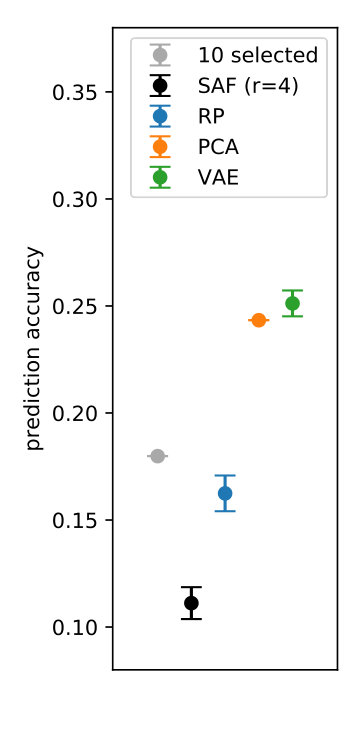 Figure 1
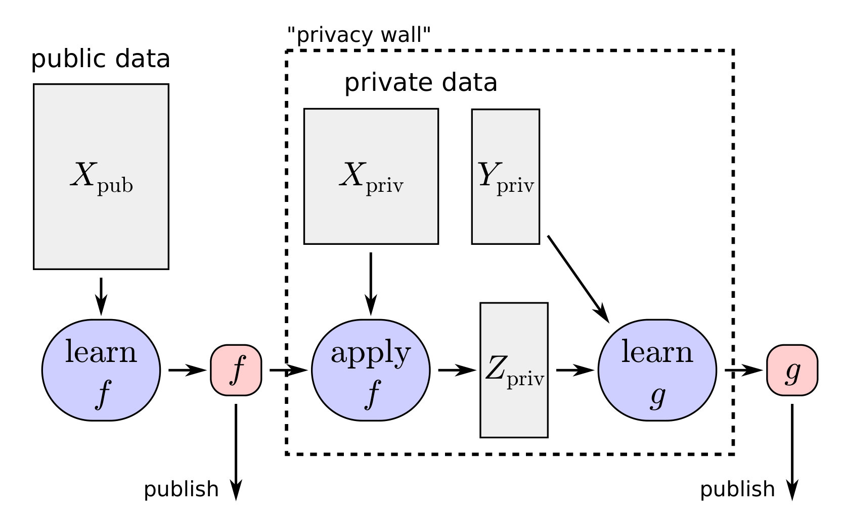 Figure 2
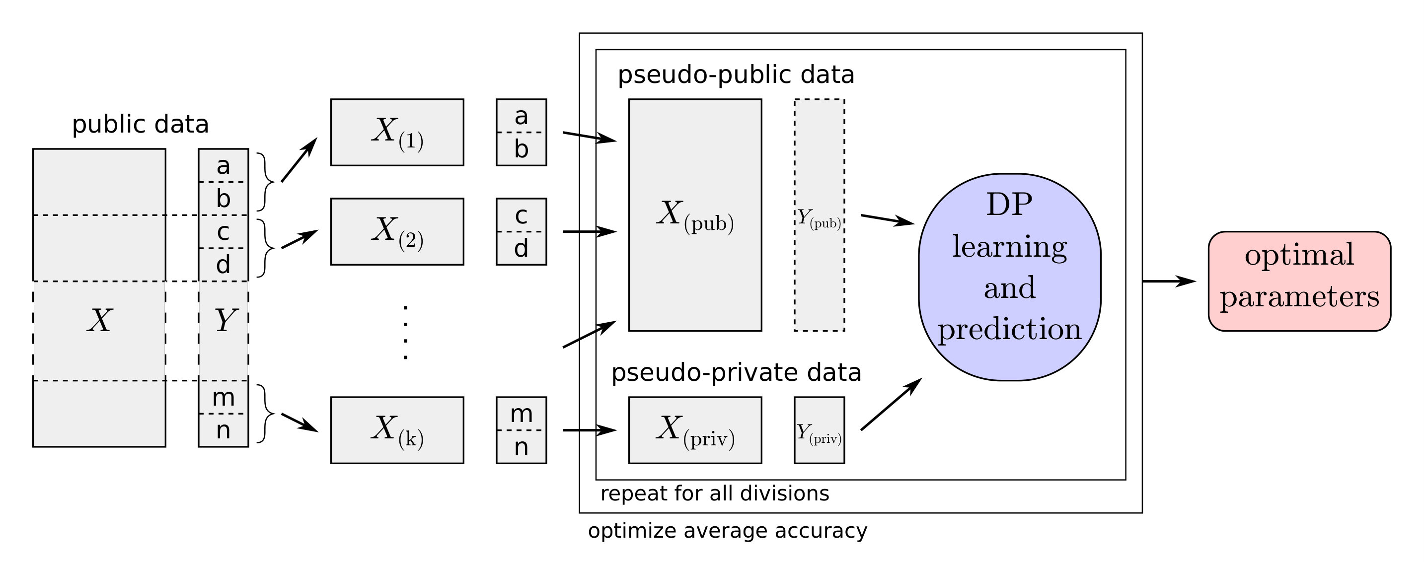 Figure 3
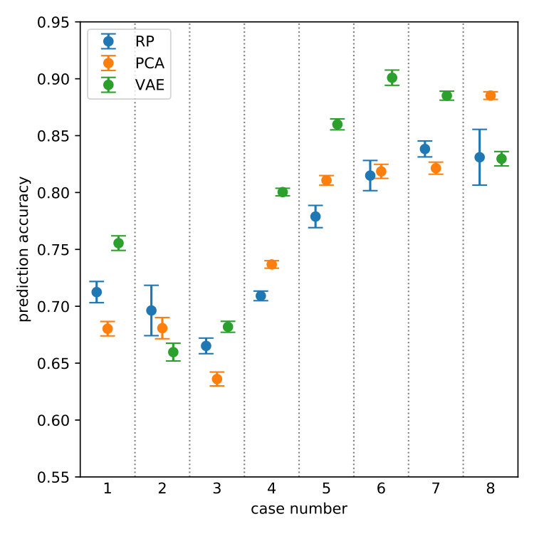 Figure 4
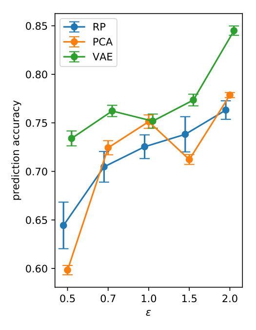 Figure 5
| Case | First cancer type | Second cancer type |
|---|---|---|
| 1 | lung squamous cell carcinoma | head & neck squamous cell carcinoma |
| 2 | bladder urothelial carcinoma | cervical & endocervical cancer |
| 3 | colon adenocarcinoma | rectum adenocarcinoma |
| 4 | stomach adenocarcinoma | esophageal carcinoma |
| 5 | kidney clear cell carcinoma | kidney papillary cell carcinoma |
| 6 | glioblastoma multiforme | sarcoma |
| - | adrenocortical cancer | uveal melanoma |
| - | testicular germ cell tumor | uterine carcinosarcoma |
| - | lung adenocarcinoma | pancreatic adenocarcinoma |
| 7 | ovarian serous cystadenocarcinoma | uterine corpus endometrioid carcinoma |
| - | brain lower grade glioma | pheochromocytoma & paraganglioma |
| - | skin cutaneous melanoma | mesothelioma |
| - | liver hepatocellular carcinoma | kidney chromophobe |
| 8 | breast invasive carcinoma | prostate adenocarcinoma |
| - | acute myeloid leukemia | diffuse large B-cell lymphoma |
| - | thyroid carcinoma | cholangiocarcinoma |
| RP | PCA | VAE | ||||
|---|---|---|---|---|---|---|
| case | repr-dim | log-lr | layers | layer-dim | ||
| 1 | 7 | 10 | 5 | -3.5 | 1 | 755 |
| 2 | 7 | 14 | 5 | -4.8 | 1 | 1925 |
| 3 | 8 | 10 | 5 | -5.3 | 2 | 2370 |
| 4 | 8 | 14 | 5 | -5.3 | 2 | 1270 |
| 5 | 7 | 8 | 4 | -4.3 | 1 | 260 |
| 6 | 8 | 10 | 5 | -4.5 | 1 | 330 |
| 7 | 7 | 12 | 5 | -3.7 | 2 | 1510 |
| 8 | 5 | 7 | 4 | -3.8 | 1 | 88 |
| RP | PCA | VAE | ||||
|---|---|---|---|---|---|---|
| repr-dim | log-lr | layers | layer-dim | |||
| 0.5 | 5 | 5 | 5 | -4.6 | 1 | 725 |
| 0.7 | 6 | 14 | 5 | -4.6 | 1 | 880 |
| 1 | 14 | 14 | 5 | -4.1 | 1 | 395 |
| 1.5 | 9 | 9 | 5 | -4.9 | 1 | 1570 |
| 2 | 10 | 11 | 10 | -4.0 | 1 | 680 |
Peer Reviews
No public reviews on file for this paper yet. If you reviewed it on a platform where reviews are public (OpenReview, ICLR, NeurIPS, ICML), you can paste yours below so the community can read it here.
Videos
No videos yet. Explain this paper in a talk, walkthrough, or lecture? Add one.
Representation Transfer for Differentially Private Drug Sensitivity Prediction
Teppo Niinimäki 1
Mikko Heikkilä 2
Antti Honkela *2,3,4,*111These authors jointly supervised the work.
and Samuel Kaski 1,∗
1Helsinki Institute for Information Technology HIIT
Department of Computer Science
Aalto University
Finland
2Helsinki Institute for Information Technology HIIT
Department of Mathematics and Statistics
University of Helsinki
Finland
3Department of Public Health
University of Helsinki
Finland and
4Helsinki Institute for Information Technology HIIT
Department of Computer Science
University of Helsinki
Finland
Abstract
Motivation: Human genomic datasets often contain sensitive information that limits use and sharing of the data. In particular, simple anonymisation strategies fail to provide sufficient level of protection for genomic data, because the data are inherently identifiable. Differentially private machine learning can help by guaranteeing that the published results do not leak too much information about any individual data point. Recent research has reached promising results on differentially private drug sensitivity prediction using gene expression data. Differentially private learning with genomic data is challenging because it is more difficult to guarantee the privacy in high dimensions. Dimensionality reduction can help, but if the dimension reduction mapping is learned from the data, then it needs to be differentially private too, which can carry a significant privacy cost. Furthermore, the selection of any hyperparameters (such as the target dimensionality) needs to also avoid leaking private information.
Results: We study an approach that uses a large public dataset of similar type to learn a compact representation for differentially private learning. We compare three representation learning methods: variational autoencoders, PCA and random projection. We solve two machine learning tasks on gene expression of cancer cell lines: cancer type classification, and drug sensitivity prediction. The experiments demonstrate significant benefit from all representation learning methods with variational autoencoders providing the most accurate predictions most often. Our results significantly improve over previous state-of-the-art in accuracy of differentially private drug sensitivity prediction.
1 Introduction
Privacy-preserving machine learning has the potential to enable the research use of many sensitive datasets, that would otherwise be out of reach for the community. This is especially the case for medical data, which almost always contain sensitive information traceable back to the data subjects. As an example, it has been shown that individuals can be identified from genomic data (Gymrek et al., 2013) including mixtures from several individuals (Homer et al., 2008). It is likely that functional genomics data such as gene expression data are also identifiable. While different anonymisation strategies (Sweeney, 2002; Machanavajjhala et al., 2007; Li et al., 2007) can protect the privacy of the data subjects to some degree, they do not have formal guarantees and can fail to provide sufficient protection in practice (Ganta et al., 2008).
Differential privacy (DP) (Dwork et al., 2006; Dwork and Roth, 2014) is a framework that guarantees strict bounds for the amount of leaked private information, even in the presence of arbitrary side information. The guarantees are obtained by adding specific forms of randomisation to the computation process. In a machine learning context this usually means adding noise either directly to the input of the algorithm (input perturbation), to the output (output perturbation), or modifying the algorithm itself, for instance, by perturbing the optimisation objective (objective perturbation).
The privacy guarantee is controlled by a “privacy budget” parameter, usually denoted by ; smaller means stricter guarantees, and can be achieved by increasing the amount of noise. Formally, a randomised mechanism is said to be -differentially private, if for all pairs of neighbouring datasets differing222There are two slightly different definitions of neighbouring datasets. In bounded case, the value of one sample is allowed to change. In unbounded case, the addition or removal of one sample is allowed. Unbounded -DP guarantee implies bounded -DP guarantee. This article uses the bounded case. on a single sample and all measurable subsets of possible outputs,
[TABLE]
Intuitively, this means that changing one sample in the dataset can change the output distribution only by a factor .
As an extension, is said to be (, )-differentially private, if
[TABLE]
for all measurable and all neighbouring datasets . The condition with nonzero is often easier to achieve than pure -DP.
In this article we are interested in DP learning for drug sensitivity prediction using gene expression data. First proposed by Staunton et al. (2001), the drug sensitivity prediction problem has attracted significant attention recently, including from a DREAM challenge in 2012 (Costello et al., 2014) that provided standardised evaluation metrics. The scale of the cytotoxicity assays needed has kept the sizes of the available data sets relatively small from a machine learning perspective. Honkela et al. (2018) were the first to apply DP learning to this problem. They needed to specifically limit the sensitivity of the learning and the dimensionality of the input data to make the learning feasible.
In abstract terms, our goal in this problem is DP learning of predictive models with high-dimensional input data, where both input and output variables need DP protection. This is a case where DP methods tend to run into trouble with moderate dataset sizes: the amount of noise that needs to be added usually increases quickly with the dimensionality, leading to output that is dominated by the noise. This warrants the use of dimensionality reducing methods with the aim of finding a good low-dimensional representation of the original data. However, unless one uses a random projection or some other “dummy” method that does not depend on the data, finding a good representation can also leak private information. For this reason, the dimension reduction method itself would also need to be made differentially private, which can completely invalidate the noise magnitude savings obtained in any downstream task like prediction.
Different solutions have been proposed for various special cases: Kifer et al. (2012) solve sparse linear regression problems by using an -DP feature selection algorithm. Honkela et al. (2018) utilise external knowledge to select a relevant subset of features. Kasiviswanathan and Jin (2016) show theoretical results on using random projections to improve DP learning on high-dimensional problems. Differentially private versions of methods such as PCA (Chaudhuri et al., 2012; Dwork et al., 2014) or deep learning (Abadi et al., 2016; Acs et al., 2018) exist and could be used to learn a representation, but the noise cost can be impractically large for small but high-dimensional datasets.
We study a straightforward solution based on feature representation transfer, similar to self-taught learning of Raina et al. (2007). By using an additional non-sensitive dataset to learn the representation, we can apply more advanced representation learning methods. This approach has many advantages: we do not need labels for the additional data set, although in our case we make use of labels for a different task; and only the main learning algorithm needs to be differentially private, while the representation can be learned using any non-DP method. Additionally, the public data can also be used for optimising any hyperparameters for the representation learning. In this article, we consider PCA and variational autoencoders.
Differentially private transfer learning was recently considered by Wang et al. (2019) in a hypothesis transfer setting, where models trained on several related source domains are used to improve learning in the desired target domain. While related, this approach is not directly applicable to our problem because the setup is different.
Another related approach was considered by Papernot et al. (2017), who propose differentially private semi-supervised knowledge transfer that uses an ensemble of “teacher” models trained on private data to label unlabeled public data, which is then used to train a “student” model that will be released. The method is flexible in a sense that it can use any “black-box” model as teachers and student. However, it is limited to classification tasks. In addition, it seems to require a rather large private dataset in addition to a small public dataset—a setting that is somewhat different from what we are interested in.
Yet another strategy is to learn a differentially private unsupervised generative model for the data (including the target variable for the prediction task of interest), use it to generate a synthetic version of the data, and use a non-DP algorithm for the actual learning task of interest. Several methods have been proposed for differentially private data sharing (Zhang et al., 2017; Xie et al., 2018; Acs et al., 2018) that could be used for generative model learning and data generation. For the problem we are considering, however, this approach is problematic as it requires solving a more general and difficult learning task, good solution of which would typically require orders of magnitude more private data than a direct solution of the original prediction task.
The rest of this article is organised as follows: In Section 2 we formalise the problem setting and give an overview of our proposed approach. Section 3 gives more details on the implementation of different parts of the proposed approach. And finally, in Section 4 we conduct experiments with the approach on two different prediction tasks on genomic data.
2 Approach
We assume a setting where we have a private dataset containing a high-dimensional feature matrix and an target vector , where is the number of samples and is the number of features. The goal is to learn a differentially private predictor from to . As learning to predict from high-dimensional directly is typically not feasible, with moderate sample size and a reasonable privacy budget, we opt for using public data to learn a low-dimensional representation for . Therefore, we also assume a publicly available dataset of an feature matrix and an auxiliary target vector for a related auxiliary prediction task. While a representation can be learned with only, the availability of is useful for selecting the size of the representation and any other hyperparameters.
We make the following informal assumptions about the relation of the public and the private data: (1) and contain the same set of features and are either draws from the same distribution or otherwise distributed similarly enough that using the same mapping to compute a representation is reasonable. (2) may or may not be of the same type as , but the prediction tasks should resemble each other enough that the prediction of can be used for optimising the hyperparameters for the main task of predicting .
We propose the following procedure:
Use the public data to learn a dimension-reducing representation mapping , where , such that . 2. 2.
Obtain a low-dimensional representation of the private feature data by applying to . 3. 3.
Learn a differentially private predictor such that . 4. 4.
Publish .
An overview of the learning process is shown in Figure 1.
It is easy to see that the proposed process has the same DP-guarantees as the learning algorithm of step 3:
Theorem 1**.**
If step 3 is -DP w.r.t. and , then the whole process is also -DP w.r.t and .
Proof.
As the learning of does not use private data, it does not leak any private information. Since each row of depends only on the corresponding row of , -guarantees w.r.t. translate directly to guarantees w.r.t. . ∎
In the following section we give some methods that can be used to implement the DP predictor and the representation mapping . In addition, we describe a procedure for tuning the hyperparameters of .
3 Methods
3.1 Differentially private prediction
Later in Section 4 we will consider prediction tasks that are either real-valued regression or binary classification tasks. Linear regression will be applied to the former and logistic regression to the latter. For now, denote by the feature matrix and by the prediction target vector (either real-valued or binary )
Logistic regression can be made differentially private with objective perturbation. The usual non-DP version of the problem can be solved by minimising the regularised negative log-likelihood with respect to the weight vector , where and denote the th sample in and respectively and controls the strength of regularisation. In a method presented by Chaudhuri and Monteleoni (2009), -DP privacy is obtained by adding a random bias term (where is a random vector drawn from a distribution with density proportional to ) to the optimisation objective. The method requires that the samples in the input feature data are bounded into a 1-sphere.
Like DP logistic regression, also a DP linear regression algorithm can be obtained with an analogous objective perturbation method (Kifer et al., 2012). However, since the underlying model belongs to the exponential family, there is also an alternative output-perturbation based -DP method that does not require iterative optimisation: Compute the sufficient statistics (, and ) and add noise to them via the Laplace-mechanism (Foulds et al., 2016). We use Bayesian linear regression with sufficient statistic perturbation and data clipping as described by Honkela et al. (2018).
3.2 Representation learning
Random projection (see e.g. Bingham and Mannila, 2001) projects the -dimensional data to an -dimensional subspace by multiplying it with a random projection matrix. This transformation has been shown to preserve approximately the distances between data points (Johnson and Lindenstrauss, 1984), which is often a desired property for dimensionality reduction methods.
Principal component analysis (PCA) finds an orthogonal linear transformation that converts the data to coordinates that are uncorrelated and whose variance decreases from first to last coordinate. When used for dimensionality reduction, only the first coordinates are kept—these correspond to the orthogonal directions in which the variance of the original data is the highest.
Variational autoencoder (VAE) (Kingma and Welling, 2014) learns a generative decoder model , where is a latent representation of , and an encoder model that approximates the posterior distribution . Both and are implemented as neural networks (typically MLPs) and optimised concurrently with variational inference.
We fix to be low-dimensional, in which case the learned encoder can be used for dimensionality reduction by setting . (As usual, define as a multivariate Gaussian distribution parametrised by mean and diagonal covariance , in which case .)
3.3 Optimisation of hyperparameters
For selecting the dimension of the representation and any other hyperparameters of the representation-learning algorithm, we propose a combination of any parameter optimisation approach (such as Bayesian optimisation, random search or grid search) and a cross-validation-like procedure for optimising an auxiliary task of predicting from . As no private data are used, the parameter optimisation phase does not consume any of the available privacy budget. In addition, if the auxiliary prediction task uses the same method as the main prediction task, then the hyperparameters could be optimised at the same time.
First the (public) data are divided into disjoint subsets. Instead of using one of the subsets as “validation” data and the rest as “training” data as in cross-validation, we use one of the subsets to simulate the private data and the rest to simulate the public data. From now on, these are referred to as pseudo-private and pseudo-public sets. The proposed framework (from Section 2) is then applied to these, that is, a representation mapping is learned from the pseudo-public data, is applied to the features of pseudo-private data, a predictor is learned for the pseudo-private target variable and its accuracy is measured. As in -fold cross-validation, this is repeated for all possible selections of the pseudo-private subset. For measuring the accuracy of , (actual) cross-validation can be used, i.e., the pseudo-private data can be further divided into different learning and validation sets.
To mimic the case in which the public and private data do not have exactly the same distribution, we also want the pseudo-public and pseudo-private data to be sufficiently different. This guides the optimiser towards selecting conservative hyperparameters that are more likely to work well on a wide range of different private datasets. If the auxiliary prediction task is classification and has multiple classes, the subset division can be based on the classes: Form each subset by selecting the samples from two (or more) classes. This strategy is based on the assumption that samples belonging to different classes have different distributions. Otherwise, for instance clustering (based on either , or both) could be used for finding a good subset division. An overview of the proposed hyperparameter optimisation method is shown in Figure 2.
4 Results
We conducted experiments with two prediction tasks using cancer cell line gene expression data: cancer type classification and drug sensitivity prediction.
4.1 Representation learning for DP cancer type classification
We first demonstrate the method by classifying TCGA pan-cancer samples according to the annotated cancer type (e.g. lung squamous cell carcinoma) using RNA-seq gene expression data. In this task we use the data from The Cancer Genome Atlas (TCGA) project (The TCGA authors, 2016) as both the private and public datasets. We use this example because it can be performed within the large TCGA dataset. Because most cancer type pairs are quite easy to identify, we focus on a number of most difficult pairs.
We used preprocessed TCGA pan-cancer RNA-seq data available at https://xenabrowser.net/datapages/. After further preprocessing (filtering out low-expression genes, applying RLE normalisation) the dataset contains 10534 samples, 14796 genes and 33 distinct cancer types. We pick two cancer types as private data and the remaining cancer types form the public dataset. The main and auxiliary prediction tasks are therefore both cancer type classification tasks, but for distinct classes. For prediction we use the differentially private logistic regression algorithm by Chaudhuri and Monteleoni (2009).
While the split to private and public data could be done in multiple ways, the prediction task would be quite easy in many of those. Hence, we use the following procedure to produce several of these splits: (1) Consider all possible splits and run a non-DP version of the pipeline (as in Figure 1) with PCA-based reduction to eight-dimensional space. (2) Build a sequence of cancer-type pairs by picking the pair that was the hardest to predict (i.e. has lowest classification accuracy), then from the remaining cancer types again the pair that was hardest, and so on. The result is a sequence of 16 pairs ordered by the prediction difficulty (see Table 1). (3) Of these pairs, select the 6 hardest, as well as those 2 of the remaining pairs that had at least 200 samples in both classes.
The full testing pipeline, including the hyperparameter optimisation phase, was then run separately for each of the 8 selected pairs as a private dataset. In each case, the remaining 15 pairs form the subsets that were used for optimising the hyperparameters.
Methods
We compare three different representation learning methods: random projection (RP), principal component analysis (PCA) and variational autoencoder (VAE) (Kingma and Welling, 2014). VAE was implemented with PyTorch (Paszke et al., 2017) and uses 1–3 hidden layers with ReLU activation functions for both the encoder and the decoder. The learning phase uses the Adam optimiser (Kingma and Ba, 2015) and is given one hour of GPU time with early stopping. The size of the representation (for RP, PCA and VAE) and other hyperparameters for VAE (the number of layers, layer sizes, learning rate) are optimised with GPyOpt (The GPyOpt authors, 2016). We also experimented with optimising a much larger set of hyperparameters, 12 in total, but GPyOpt had difficulties in obtaining similar levels of performance.
For each of the 8 test cases we ran the hyperparameter optimisation phase once, giving it 5 days of time. Then with the best found hyperparameters we ran the final testing 9 times with different RNG seeds, and report the mean prediction accuracy as well as the standard deviation of the mean. In measuring the prediction accuracy (both for hyperparameter optimisation and for final testing) we use 10-fold cross-validation.
Results
Figure 3 shows the final prediction accuracy in the selected 8 cases for . While none of the methods fully dominates the others, VAE seems to get some edge, being clearly the best in about half of the cases and doing decent job in the rest of the cases too. The selected hyperparameters are listed in Table 2. Interestingly, VAE seems to always end up with lower dimensionality of the representation than the other two methods. This could be due to the fact that VAE allows nonlinear transformations which can help to compress the relevant information in the data into a smaller number of dimensions. On the other hand, it is not clear why RP also always chooses lower dimension than PCA.
The prediction accuracy as a function of in the case 1 is shown in Figure 4 and the corresponding hyperparameters are shown in Table 3. As expected, larger results in better accuracy. There is some variability compared to case 1 in Figure 3, which is mostly likely due to the results having been computed with different hyperparameters. Due to the high computational cost, variability due to hyperparameter adaptation is not included in the error bars.
4.2 Representation learning for DP drug sensitivity prediction
Our main learning task is to predict the sensitivities of cancer cell lines to certain drugs. In this task we use data from the Genomics of Drug Sensitivity in Cancer (GDSC) project (Yang et al., 2013) as private data. After preprocessing the data contains 985 samples, 11714 genes and 265 drugs. The data are sparse in the sense that not all drugs have been tested on all samples. For prediction we use the differentially private Bayesian linear regression algorithm by Honkela et al. (2018). The DP linear regression is applied for each drug separately, using the full budget as if it was the only drug we are interested in. We then measure and report the average prediction accuracy over all drugs.
As public data we use the gene expression measurements from the TCGA data with cancer type classification as the auxiliary prediction task. The private and public datasets are unified by removing genes not appearing in both datasets. In addition, since the TCGA gene expression data are RNA-seq-based while GDSC data are based on microarrays, we apply quantile normalisation to each gene in the TCGA data to make it match the distribution of the gene in the GDSC data. (While this operation theoretically breaks the privacy guarantees, in practice we can avoid the issue by assuming that the expression distributions obtained with the microarray technology are public knowledge.)
Methods
In addition to RP, PCA and VAE, we also compare to DP feature selection by Sample and Aggregate framework (SAF) as presented by Kifer et al. (2012), as well as to using a set of 10 preselected genes that were used by Honkela et al. (2018) in the same prediction task. In the case of SAF half of the privacy budget is reserved for feature selection.
RP, PCA and VAE learning was performed in a similar manner as in the cancer type classification task. For selecting the size of the representation of SAF, we simply ran it with all possible sizes and select the best result (which is obviously unfair for the other methods and would yield a weaker privacy guarantee).
Results
Figure 5 shows the average prediction performance, measured by Spearman’s rank correlation. Here PCA and VAE are the best by some margin, both improving significantly over the previous state-of-the-art with preselected genes. On the other hand, SAF is clearly the worst as the DP feature selection is essentially random due to small privacy budget, and since it leaves only half of the privacy budget for the main prediction task.
5 Discussion
Our results clearly demonstrate that representation learning with public data can significantly improve the accuracy of differentially private learning, compared to using a set of preselected dimensions or doing differentially private feature selection. Whether it is beneficial to use more advanced representation learning methods such as variational autoencoders instead of simple methods such as PCA or random projections, depends on the task. On some tasks that certainly seems to be the case.
In our current approach, the representation is learned in an unsupervised manner and the auxiliary supervised task is only used for hyperparameter selection. A natural question, that we leave for further work, is whether representation learning would also benefit from having an integral auxiliary prediction task that would be learned concurrently with the representation. The optimisation target would in that case be a combination of unsupervised reconstruction error and supervised prediction error. This approach would require an auxiliary target variable, as is the case in this work with hyperparameter optimisation.
In general, we believe DP learning can be important in opening genomic and other biomedical datasets to broader use. This can significantly advance open science and open data, and lead to more accurate models for precision medicine. So far, the accuracy of DP learning in most practical applications is not comparable to realistic non-private alternatives. Our present work makes an important contribution toward making DP learning practical.
In the present work the representation learning was not performed under DP. This is a clear limitation if the other data set also needs privacy protection. This can in theory be addressed easily, by simply training the representation model under DP, but this will likely have an impact on the accuracy of the final model. Ultimately we believe that a clever combination of private and non-private data such as in our paper can lead to the best results.
Acknowledgements
We thank the reviewers of an earlier workshop version of this article for helpful comments.
Funding
This work has been supported by the Academy of Finland [Finnish Center for Artificial Intelligence FCAI and grants 292334, 294238, 303815, 303816, 313124].
The reference list from the paper itself. Each links out to its DOI / PubMed record.
- 1Abadi et al. (2016) Abadi, M., Chu, A., Goodfellow, I., Mc Mahan, H. B., Mironov, I., Talwar, K., and Zhang, L. (2016). Deep learning with differential privacy. In Proc. 2016 ACM SIGSAC Conf. on Computer and Communications Security (CCS 2016) , pages 308–318.
- 2Acs et al. (2018) Acs, G., Melis, L., Castelluccia, C., and Cristofaro, E. D. (2018). Differentially private mixture of generative neural networks. IEEE Trans. Knowl. Data Eng. doi:10.1109/TKDE.2018.2855136.
- 3Bingham and Mannila (2001) Bingham, E. and Mannila, H. (2001). Random projection in dimensionality reduction: Applications to image and text data. In Proc. Seventh ACM SIGKDD Int. Conf. on Knowledge Discovery and Data Mining (KDD 2001) , pages 245–250.
- 4Chaudhuri and Monteleoni (2009) Chaudhuri, K. and Monteleoni, C. (2009). Privacy-preserving logistic regression. In Advances in Neural Information Processing Systems 21 , pages 289–296.
- 5Chaudhuri et al. (2012) Chaudhuri, K., Sarwate, A., and Sinha, K. (2012). Near-optimal differentially private principal components. In Advances in Neural Information Processing Systems 25 , pages 989–997.
- 6Costello et al. (2014) Costello, J. C. et al. (2014). A community effort to assess and improve drug sensitivity prediction algorithms. Nat. Biotechnol. , 32 (12), 1202–1212.
- 7Dwork and Roth (2014) Dwork, C. and Roth, A. (2014). The algorithmic foundations of differential privacy. Found. Trends Theor. Comput. Sci. , 9 (3–4), 211–407.
- 8Dwork et al. (2006) Dwork, C., Mc Sherry, F., Nissim, K., and Smith, A. (2006). Calibrating noise to sensitivity in private data analysis. In Theory of Cryptography (TCC 2006) , pages 265–284.