Global Stability analysis of a cellular model of Hepatitis C Virus infection under treatment
Alexis Nangue

TL;DR
This paper conducts a comprehensive stability analysis of a cellular model for Hepatitis C Virus infection under treatment, demonstrating global stability and boundedness of solutions using Lyapunov functions.
Contribution
It provides the first global stability proof for the HCV model under therapy, ensuring solutions are positive, bounded, and do not exhibit periodic behavior.
Findings
Solutions are global, positive, and bounded.
The model is globally asymptotically stable.
No periodic orbits are observed.
Abstract
In this paper, we present the global analysis of a HCV model under therapy. We prove that the solutions with positive initial values are global, positive, bounded and not display periodic orbits. In addition, we show that the model is globally asymptotically stable, by using appropriate Lyapunov functions.
Click any figure to enlarge with its caption.
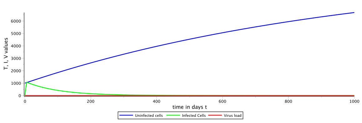 Figure 1
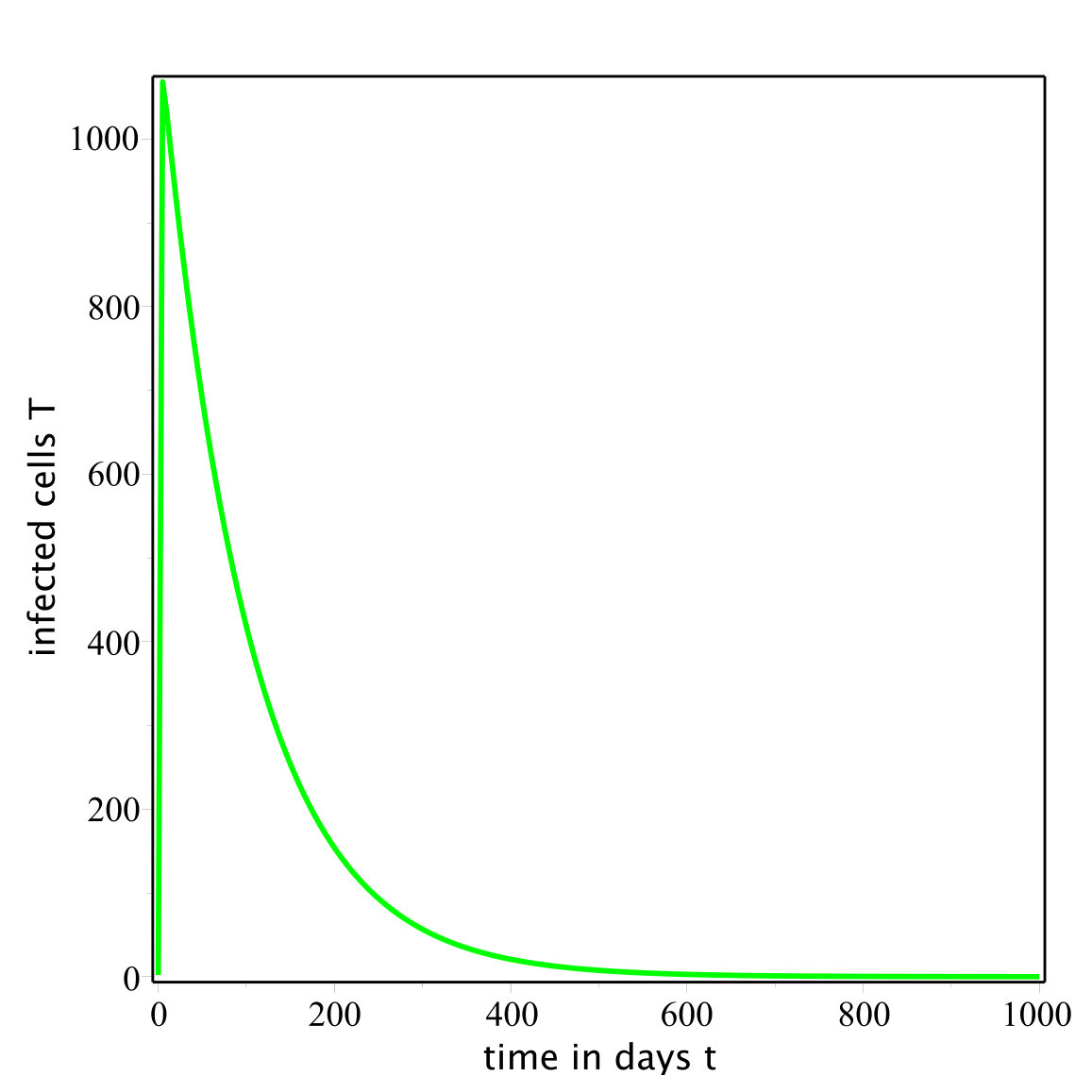 Figure 2
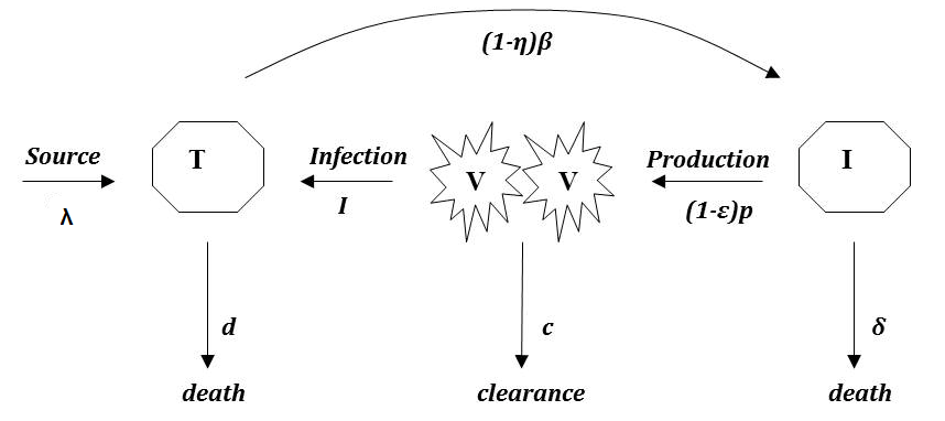 Figure 3
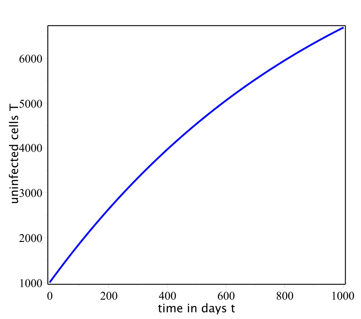 Figure 4
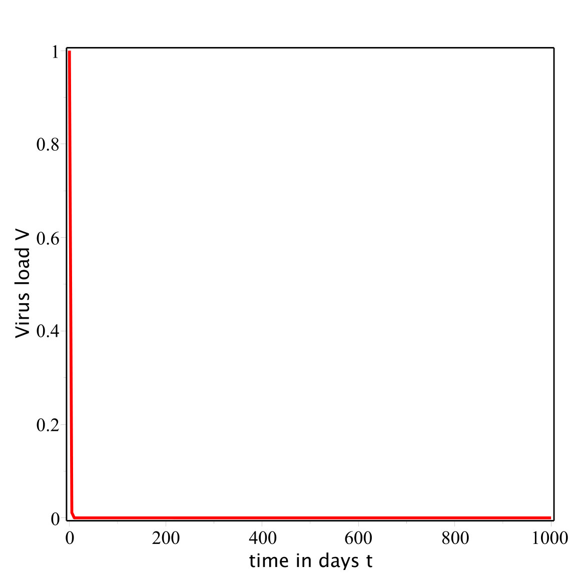 Figure 5
Peer Reviews
No public reviews on file for this paper yet. If you reviewed it on a platform where reviews are public (OpenReview, ICLR, NeurIPS, ICML), you can paste yours below so the community can read it here.
Videos
No videos yet. Explain this paper in a talk, walkthrough, or lecture? Add one.
Taxonomy
TopicsHepatitis C virus research · Mathematical and Theoretical Epidemiology and Ecology Models · Liver Disease Diagnosis and Treatment
Global stability analysis of the
original cellular model of hepatitis C Virus infection under therapy
Alexis Nangue Email : Alexis Nangue : [email protected] University of Maroua, Higher Teacher’s Training College, Department of Mathematics, P.O.Box 55 Maroua, Cameroon
Abstract
In this paper, we present the global analysis of a HCV model under therapy. We prove that the solutions with positive initial values are global, positive, bounded and not display periodic orbits. In addition, we show that the model is globally asymptotically stable, by using appropriate Lyapunov functions.
Keywords:HCV cellular model, differential system, therapy, local and global solution, invariant set, stability.
1 Introduction
According to [15] recent estimates, more than 185 million people around the world have been infected with the hepatitis C virus (HCV), of whom 350 000 die each year. One third of those who become chronically infected are predicted to develop liver cirrhosis or hepatocellular carcinoma. Despite the high prevalence of disease, most people infected with the virus are unaware of their infection. For many who have been diagnosed, treatment remains unavailable. Treatment is successful in the majority of persons treated, and treatment success rates among patients treated in low- and middle-income countries are similar to those in high-income countries Hepatitis C virus (HCV) infects liver cells (hepatocytes). Approximately 200 million people worldwide are persistently infected with the HCV and are at risk of developing chronic liver disease, cirrhosis and hepatocellular carcinoma. HCV infection therefore represents a significants global public health problem. HCV established chronic hepatitis in - of infected adults [12].
In literature, several mathematical models have been introduced for understanding HCV temporal dynamics [4, 9, 10].
In this article, we consider the basic extracellular model with therapy presented by Neumann et al. in [9]. Given the recent surge in the development of new direct acting antivirals agents for HCV therapy, mathematical modelling of viral kinetics under treatment continues to play an instrumental role in improving our knowledge and understanding of virus pathogenesis and in guiding drug development [2, 7, 11].
To proceed, we assume that the uninfected target cells are produced at a rate , die at constant rate per cell. On the other hand, the target cells are infected with de novo infection rate constant of and the infected cells die at a constant rate of per cell. The hepatitis C virions are produced inside the infected cells at an average rate per infected cell and have a constant clearance rate per virion. Thereby, viral persistence will occur when rate of viral production , de novo infection , and production of target cells exceeds the clearance rate , death rate of infected cells and target cells death rate . In addition, the therapeutic effect of IFN treatment in this model involved blocking virions production and reducing new infections which, are described in fractions and , respectively. (, ).
According to [3, 9], the above assumptions lead to the following differential equations :
[TABLE]
where the equations relate the dynamics relationship between, T as the uninfected target cells (hepatocytes), I as the infected cells and V as the viral load (amount of viruses present in the blood). In this article, model system (1) is taken as the original model used to analyse the HCV dynamics.
The initial conditions associated to system (1) are given by :
[TABLE]
This paper is organized as follows : The global properties of the solutions to the mathematical model is carried out in Section 1. The stability of the disease non-infected steady state, and the infected steady state is analysed in section 2.
2 Properties of solutions to the Cauchy problem (1),(2)
2.1 Existence of local solutions
The first step in examining model (1) is to prove that local solution to the initial-value problem does, in fact, exist, and that this solution is unique.
Theorem 2.1
Let , , be given. There exists and continuously differentiable functions , , such that the ordered triple satisfies (1) and .
Proof**.** To prove the result, we use the classical Cauchy-Lipschitz theorem. Since the first order system of ordinary differential equations (1) is autonomous, it suffices to show that the function defined by :
[TABLE]
is locally Lipschitz in its argument. In fact, it is enough to notice that the jacobian matrix
[TABLE]
is linear in and therefore locally bounded for every . Hence, H has a continuous, bounded derivative on any compact subset of and so H is locally Lipschitz in ; In addition H is continuous. By Cauchy-Lipschitz theorem, there exits a unique solution, , to the ordinary differential equation
[TABLE]
with initial value on for some time .
Remark 1
The model (1) can be rewrite in the form
[TABLE]
where and F is defined by (3).
Remark 2
Since H is a continuously differentiable function, we deduce a unique maximal solution of initial value problem (1), (2). In addition, F, being indefinitely continuously differentiable, we can also deduce that this solution is also only if indefinitely continuously differentiable.
Additionally, we may show that for positive initial data, solutions of (1), (2) remain positive as long as they exist.
2.2 Positivity
Theorem 2.2
Let be a solution of the Cauchy problem (1), (2) on an interval . Assume the initial data of (1), (2) satisfy , , and then , and remain positive for all .
Proof**.** Call the variables . If there is an index and a time for which , let be the infimum of all such for any i. Then the restriction of the solution to the interval is positive and for a certain value of . The equation for in the system (1) can be written in the form :
[TABLE]
where is non-negative. As a consequence and , . In fact :
Recall that all constants in the system (1) are non-negative. Using this and the solutions on , we have :
[TABLE]
which yields :
[TABLE]
Similarly, in one hand we have :
[TABLE]
Solving for T yields
[TABLE]
where . In other hand we have :
[TABLE]
Recall that we have a bound on T, so
[TABLE]
where . Solving the differential inequation yields :
[TABLE]
where depends upon , and only, and , . Using the fact that and are positive, (4) yields :
[TABLE]
With these bounds in place, we can now examine and bound it from below using :
[TABLE]
for , where . Shifting that last term to the other side of the equation yields :
[TABLE]
Since we know
[TABLE]
we find that for ,
[TABLE]
Therefore , for all . In particular , which is a contradiction and the theorem is proven.
Remark 3
- (i)
With this, we have a general idea that the model is sound, and can say with certainty that it remains biologically valid as long as it began with biologically-reasonable (i.e, positive) data. This also shows that once infected, it is entirely possible that the virus may continue to exist beneath a detectable threshold without doing any damage. 2. (ii)
One reason why we choose the strict inequalities for the initial data is that often in biological (or chemical) applications we are interested in the case of solutions where all unknowns are positive. This means intuitively that all elements of the model are ’active’. On the other hand it is sometimes relevant to consider solutions with non-strict inequalities. In fact the statement of the theorem with strict inequalities implies the corresponding statement with non-strict inequalities in a rather easy way.
2.3 Existence of global solutions
It will now be shown, with the help of the continuation criterion the existence of global solutions.
Theorem 2.3
The solutions of the Cauchy problem (1), (2), with positive initial data, exist globally in time in the future that is : on .
Proof**.** To prove this it is enough to show that all variables are bounded on an arbitrary finite interval . Using the positivity of the solutions is suffices to show that all variables are bounded above.
Taking the sum of equations (1a) and (1b) shows that :
[TABLE]
and hence that . Thus and are bounded on any finite interval. The third equation i.e. equation (1c), then shows that cannot grow faster than linearly and is also bounded on any finite interval.
2.4 Global boundedness of solutions
Theorem 2.4
For any positive solution of system (1), (2) we have :
[TABLE]
where
[TABLE]
Proof**.** According to equations (1a) and (1b), we have :
[TABLE]
Gronwall inequality[13] yields :
[TABLE]
[TABLE]
Another hand, from equation (1c), we have :
[TABLE]
Once more Gronwall inequality yields :
[TABLE]
Therefore the theorem is proven.
As consequences of Theorem 2.4 we have :
Remark 4
Let S be a solution of system (1). If then, the limit of exits when . In other words the solution is globally uniformly bounded in the future. In particular, S is periodic if and only if S is stationary under the condition that admits a finite limit when tends to infinity.
Theorem 2.5
Let and be a maximal solution of the Cauchy problem (1), (2)(). If and then the set :
[TABLE]
where and , is a positively invariant set by system (1).
Proof**.** Let . We shall show that :
- (i)
If then for all , . 2. (ii)
If then for all , .
- (i)
Let us suppose that there exists such that : ,
[TABLE]
Let .
Since , hence
, In addition, according to equations (1a) and (1b) of system (1) we have :
[TABLE]
which yields :
[TABLE]
hence, there exists such that for all , , a contradiction. therefore for all , . 2. (ii)
Let us suppose that there exists such that : ,
[TABLE]
Let .
Since , hence
, In addition, according to equation (1c) of system (1) we have :
[TABLE]
which yields :
[TABLE]
hence, there exists such that for all , , a contradiction. therefore for all , .
3 Stability analyses
3.1 Equilibria, Basic reproduction number and
local stability
According to [3], apart from an infection-free equilibrium
[TABLE]
the system (1) has an infected equilibrium during therapy , where :
[TABLE]
The basic reproduction number has been defined in the introduction as the average number of secondary infections that occur when one infective is introduced into a completely susceptible host population [5, 6, 14]. Note that is also called the basic reproduction ratio [5] or basic reproductive rate [1]. It is implicitly assumed that the infected outsider is in the host population for the entire infectious period and mixes with the host population in exactly the same way that a population native would mix. Following the method done by [14], we have :
Proposition 3.1
The basic reproduction number for model (1) is given by :
[TABLE]
Now we can express the components of infected equilibrium in term of . Hence (6) becomes :
[TABLE]
The following results summarize the main results regarding the local stability of the disease-free steady state , and the local stability of the infected steady state during therapy . The proof of these results can be found in [3].
Theorem 3.2
The infection-free steady state of model (1) is locally asymptotically stable if and unstable if
Theorem 3.3
The infected steady state during the therapy of model (1) is locally asymptotically stable if and unstable if
3.2 Global Stability
In this section, firstly we prove the global stability of the infection-free equilibrium of model (1) when the basic reproduction number is less than or equal to unity. And secondly we prove the global stability of infected equilibrium whenever it exists. We have seen previously[3] that the unique positive endemic equilibrium exits when the basic reproduction number is greater than or equal to unity.
Theorem 3.4
- (i)
The infection-free steady state of model (1) is globally asymptotically stable if the basic reproduction number and unstable if . 2. (ii)
The infected steady state during therapy of model (1) is globally asymptotically stable if the basic reproduction number .
Proof**.**
- (i)
Consider the Lyapunov function :
[TABLE]
is defined, continuous and positive definite for all , , . Also, the global minimum occurs at the infection free equilibrium . Further, function , along the solutions of system (1), satisfies :
[TABLE]
Further collecting terms, we have
[TABLE]
Since the arithmetical mean is greater than or equal to the geometrical mean,
[TABLE]
the function are non-positive for all . In addition, since ensures for all , . The equality holds only (a) at the free equilibrium or (b) when and . The latter case implies .
Therefore, the largest compact invariant subset of the set
[TABLE]
is the singleton . By the Lasalle invariance principle[8], the infection-free equilibrium is globally asymptotically stable if . We have seen previously that if , at least one of the eigenvalues of the Jacobian matrix evaluated at has a positive real part. Therefore, the infection-free equilibrium is unstable when .
- (ii)
Consider the Lyapunov function :
[TABLE]
The time derivative of along the trajectories of system (1) is :
[TABLE]
Collecting terms, and canceling identical terms with opposite signs, yields
[TABLE]
[TABLE]
The terms between the brackets are less than or equal to zero by the inequality (the geometric mean is less than or equal to the arithmetic mean)
[TABLE]
It should be noted that holds if and only if take the steady states values Therefore the infected equilibrium is globally asymptotically stable.
4 Numerical Simulation
Some numerical simulations have been done in the case to confirm theoretical result obtain on global stability for the uninfected equilibrium.
We run simulations using the initial conditions: , and and the following parameter values : ; ; ; ; ; ; , .
5 Conclusion
In this paper, we have extended the first part of the work done by Chong et al. in [3] where they only studied the local stability of the fundamental mathematical model of hepatitis C infection with treatment.
Acknowledgements
I am grateful to Professor Alan Rendall for valuable and tremendous discussions. I wish to thank him for introducing me to Mathematical Biology and to its relationship with Mathematical Analysis.
The reference list from the paper itself. Each links out to its DOI / PubMed record.
- 1[1] R. M. Anderson and R. M. May, eds. 1991. Infectious Diseases of Humans: Dynamics and Control , Oxford University Press, Oxford, UK.
- 2[2] Chatterjee, A., Guedj, J., & Perelson, A. S. (2012). Mathematical modelling of HCV infection: what can it teach us in the era of direct-acting antiviral agents? Antiviral Therapy, 17(6Pt B), 1171-1182. http://dx.doi.org/10.3851/IMP 2428.
- 3[3] Chong, Maureen Siew Fang, Shahrill, Masitah, Crossley, Laurie and Madzvamuse, Anotida, 2015 The stability analyses of the mathematical models of hepatitis C virus infection . Modern Applied Science, 9(3). pp. 250-271. ISSN 1913-1844.
- 4[4] Dahari, H., Lo, A., Ribeiro, R. M., & Perelson, A. S. (2007). Modeling hepatitis C virus dynamics: Liver regeneration and critical drug efficacy . Journal of Theoretical Biology, 247, 371-381. http://dx.doi.org/10.1016/j.jtbi.2007.03.006.
- 5[5] O. Diekmann, J. A. P. Heesterbeek, and J. A. J. Metz, 1990. On the definition and the computation of the basic reproduction ratio R 0 in models for infectious diseases in heterogeneous populations , J. Math. Biol., 28, pp. 365 382.
- 6[6] K. Dietz, 1988. Density dependence in parasite transmission dynamics, Parasit . Today, 4 , pp. 91 97.
- 7[7] Guedj, J., & Neumann, A. U. (2010). Understanding hepatitis C viral dynamics with direct-acting antiviral agents due to the interplay between intracellular replication and cellular infection dynamics. Journal of Theoretical Biology, 267(3), 330-340. http://dx.doi.org/10.1016/j.jtbi.2010.08.036.
- 8[8] Khalil, H., 2002. Nonlinear Systems , 3rd edn. Prentice Hall, New York.