TL;DR
This paper demonstrates that high-resolution SPH simulations with over 10^8 particles are crucial for accurately modeling giant impacts on Uranus, revealing convergence issues at lower resolutions and introducing new software tools for efficient, realistic initial conditions and simulations.
Contribution
The authors develop a novel particle placement algorithm and an advanced hydrodynamics code, SWIFT, enabling high-resolution planetary impact simulations with improved accuracy and efficiency.
Findings
Simulations with over 10^7 particles are needed for convergence of bulk properties.
Higher resolutions significantly affect the amount and distribution of ejected debris.
The new software tools are publicly available for the community.
Abstract
We perform simulations of giant impacts onto the young Uranus using smoothed particle hydrodynamics (SPH) with over 100 million particles. This 100--1000 improvement in particle number reveals that simulations with below 10^7 particles fail to converge on even bulk properties like the post-impact rotation period, or on the detailed erosion of the atmosphere. Higher resolutions appear to determine these large-scale results reliably, but even 10^8 particles may not be sufficient to study the detailed composition of the debris -- finding that almost an order of magnitude more rock is ejected beyond the Roche radius than with 10^5 particles. We present two software developments that enable this increase in the feasible number of particles. First, we present an algorithm to place any number of particles in a spherical shell such that they all have an SPH density within 1% of the…
Click any figure to enlarge with its caption.
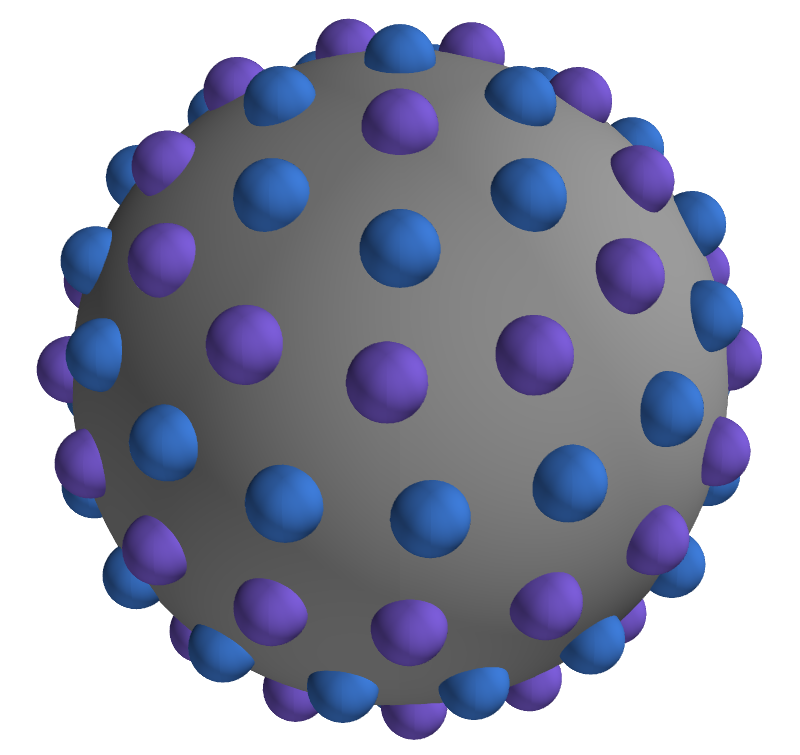 Figure 1
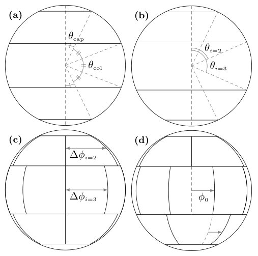 Figure 2
 Figure 3
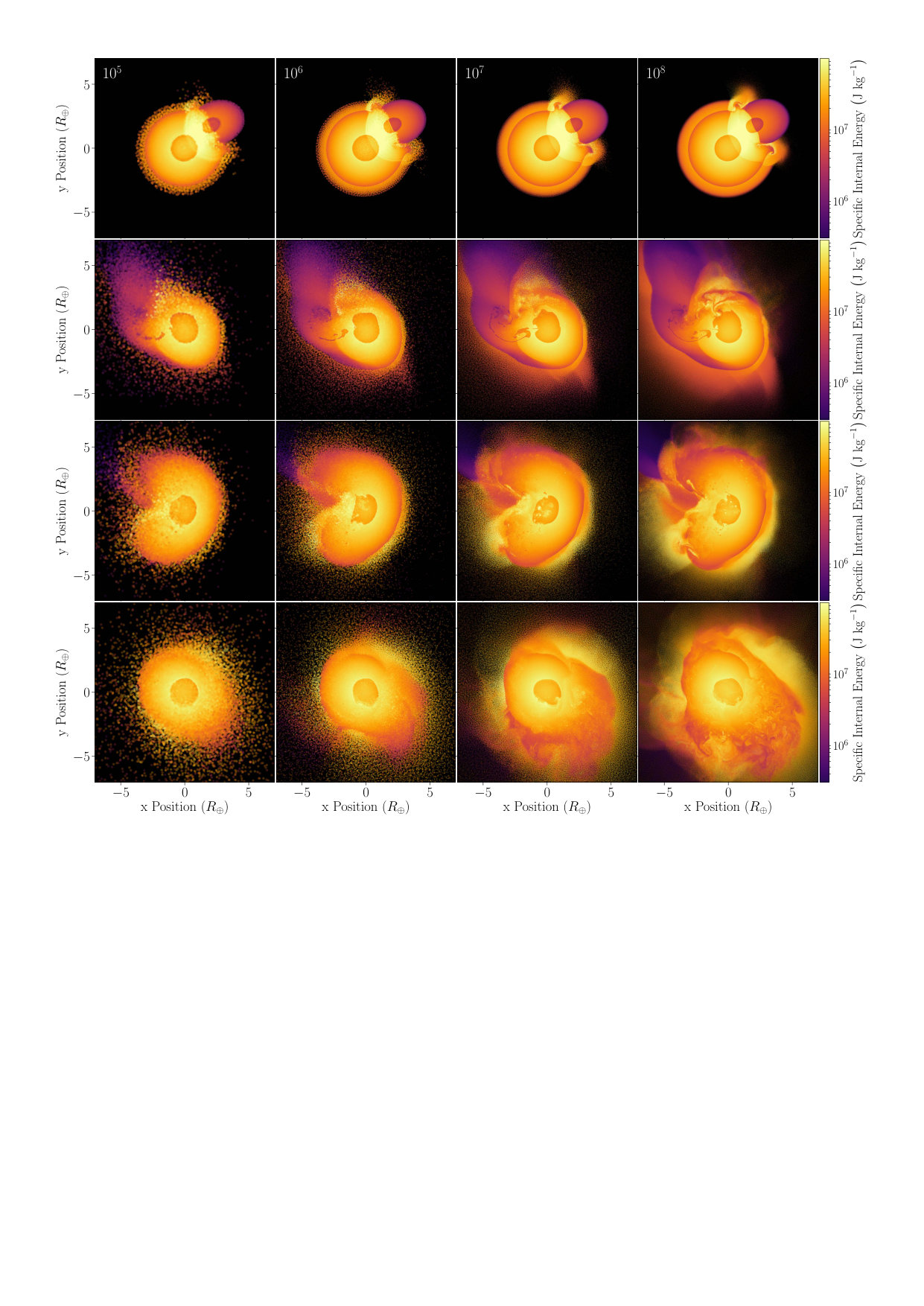 Figure 4
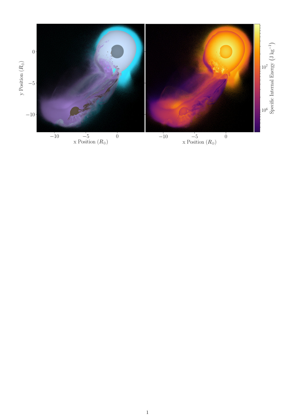 Figure 5
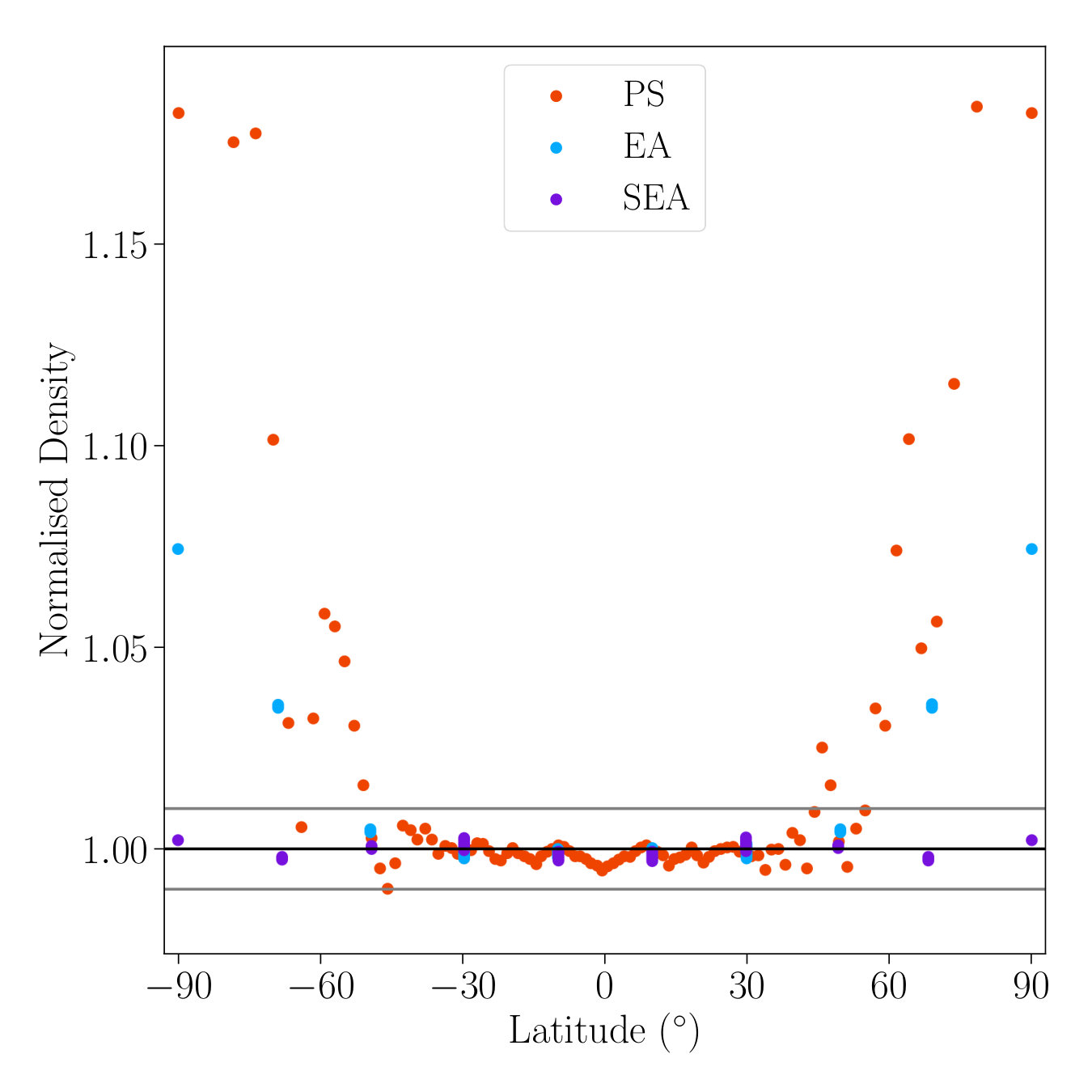 Figure 6
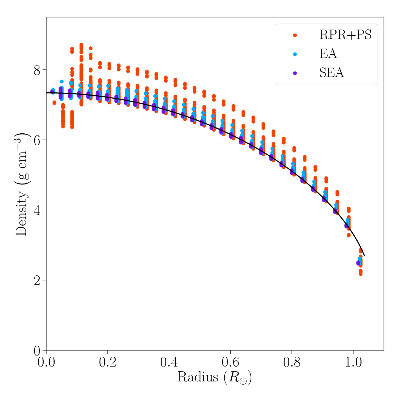 Figure 7
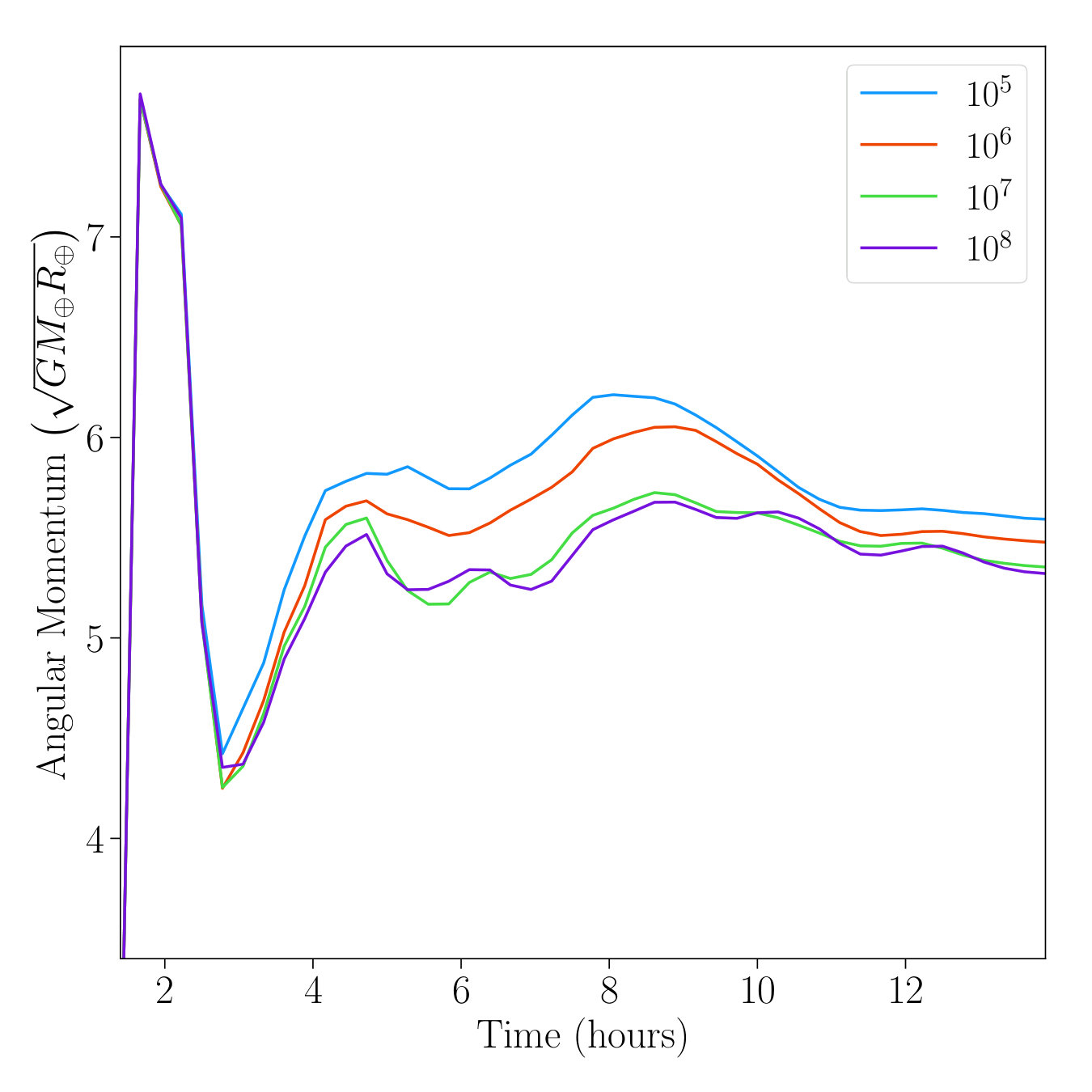 Figure 8
 Figure 9
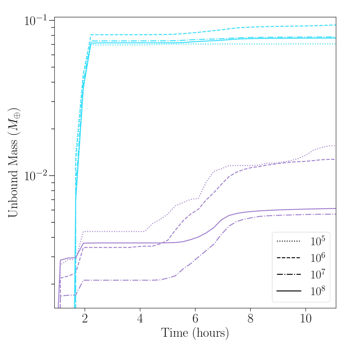 Figure 10
Peer Reviews
No public reviews on file for this paper yet. If you reviewed it on a platform where reviews are public (OpenReview, ICLR, NeurIPS, ICML), you can paste yours below so the community can read it here.
Code & Models
Videos
No videos yet. Explain this paper in a talk, walkthrough, or lecture? Add one.
Planetary Giant Impacts:
Convergence of High-Resolution Simulations using Efficient Spherical Initial Conditions and SWIFT
J. A. Kegerreis1, V. R. Eke1, P. Gonnet2, D. G. Korycansky3, R. J. Massey1, M. Schaller4, L. F. A. Teodoro5
1Institute for Computational Cosmology, Durham University, Durham, DH1 3LE, UK
2Google AI Perception, Google Switzerland, 8002 Zurich, Switzerland
3CODEP, Earth Sciences, University of California, Santa Cruz, CA, USA
4Leiden Observatory, Niels Bohrweg 2, 2333 CA Leiden, Netherlands
5BAERI/NASA Ames Research Center, Moffett Field, CA, USA [email protected]
(Accepted XXX. Received YYY; in original form ZZZ)
Abstract
We perform simulations of giant impacts onto the young Uranus using smoothed particle hydrodynamics (SPH) with over 100 million particles. This – improvement in particle number reveals that simulations with below particles fail to converge on even bulk properties like the post-impact rotation period, or on the detailed erosion of the atmosphere. Higher resolutions appear to determine these large-scale results reliably, but even particles may not be sufficient to study the detailed composition of the debris – finding that almost an order of magnitude more rock is ejected beyond the Roche radius than with particles. We present two software developments that enable this increase in the feasible number of particles. First, we present an algorithm to place any number of particles in a spherical shell such that they all have an SPH density within 1% of the desired value. Particles in model planets built from these nested shells have a root-mean-squared velocity below 1% of the escape speed, which avoids the need for long precursor simulations to produce relaxed initial conditions. Second, we develop the hydrodynamics code SWIFT for planetary simulations. SWIFT uses task-based parallelism and other modern algorithmic approaches to take full advantage of contemporary supercomputer architectures. Both the particle placement code and SWIFT are publicly released.
keywords:
methods: numerical – hydrodynamics – planets and satellites: physical evolution – planets and satellites: atmosphere
††pubyear: 2019††pagerange: Planetary Giant Impacts: Convergence of High-Resolution Simulations using Efficient Spherical Initial Conditions and SWIFT –B
1 Introduction
Giant impacts are thought to dominate many planets’ late accretion and evolution. We see the consequences of these violent events on almost every planet in our solar system, from the formation of Earth’s Moon to the odd obliquity of Uranus spinning on its side. As such, they are expected to play a similarly important role in the evolution of the many exoplanetary systems that are now being observed in detail. These complicated and highly non-linear processes are most commonly studied using smoothed particle hydrodynamics (SPH) simulations (e.g. Benz et al., 1986).
SPH is a Lagrangian (particle-based) method used in a wide range of topics in astrophysics and many other fields, from planetary impacts and supernovae to galaxy evolution and cosmology (Springel, 2010; Monaghan, 2012). As well as correctly evolving the simulation particles with time, it is crucial to start from appropriate initial conditions for any model’s evolution to accurately reflect its real-world counterpart. Furthermore, enough particles must be used to resolve the physical processes in sufficient detail, and recent work has shown that standard-resolution simulations ( to particles) can produce unreliable results that have not converged numerically (Hosono et al., 2017; Genda et al., 2015). This motivates the pursuit of simulation codes that can take full advantage of contemporary supercomputing architectures, enabling more particles to be used to run suitable convergence tests and, hopefully, simulations with sufficiently high resolution.
Towards this end, we present the simple SEA111 The SEAGen code is publicly available at github.com/jkeger/seagen and the python module seagen— can be installed directly with pip.
scheme for creating optimal spherical arrangements of particles (§2.1, §3.1) and the hydrodynamics code SWIFT222 SWIFT is in open development and is publicly available at www.swiftsim.com.
that we have developed to run planetary impact (and cosmological) simulations (§2.2). We use these tools to model giant impacts onto a young Uranus at high resolution using over SPH particles, and test the convergence of various physical properties with increasing particle number (§1.2, §3.2). We then present conclusions in §4.
1.1 Particle Placement and Initial Conditions
Many problems in astrophysics feature spherical symmetry, such as those involving stars or planets. Before one can simulate and study these problems with a particle-based method like SPH, each initial object must first be converted into an appropriate set of particles. Two common approaches to creating arrangements of SPH particles in spheres are: (1) to use a lattice that can be distorted until it approximately matches the required shape and densities; and (2) to relax an imperfect initial state into a fully settled one with a pre-production simulation.
A third, more recent approach is to arrange the particles analytically while accounting for the spherical symmetry from the outset, by placing particles in nested spherical shells (Saff & Kuijlaars, 1997; Raskin & Owen, 2016; Reinhardt & Stadel, 2017). These methods aim to combine the minimal computation required for lattice methods with the settled and symmetric properties of simulated glasses. We present a comparable scheme that further ensures every particle’s SPH density is within 1% of the desired value. This leads to initial conditions that are quick and simple to produce, close to equilibrium, and in which every particle has a realistic density and, therefore, pressure.
Lattice-based methods are popular because they are easy to implement and, since the inter-particle separations are uniform by construction, they can accurately match a simple density profile. This can be achieved either by stretching the lattice radially or by varying the particle mass – although keeping the masses of all particles very similar is usually desirable. However, the grid-like properties of a lattice introduce unwanted anisotropies to a problem and may be unstable to perturbations (Herant, 1994; Morris, 1996; Lombardi et al., 1999).
Furthermore, a spherically symmetric object like a planet or star features important boundaries at specific radii. Both the outer surface and internal layers require discontinuities in density and material. The particles in a lattice are dispersed at all radii, so cannot reproduce such sharp changes at these boundaries. A similarly quick and simple alternative to lattice methods is to randomly place particles following an appropriate probability distribution function, either restricted in nested shells or anywhere in the sphere. However, these methods are noisy and result in extreme variations in local particle densities.
In SPH, the density of a particle is estimated by summing the masses of typically 50 nearby ‘neighbour’ particles, weighting by a 3D-Gaussian-shaped kernel that decreases the contribution of more-distant neighbours. Thus a particle that is placed too close to another will have a higher density and not be in equilibrium. The accuracy of every particle’s density is important because of how stiff the equation of state (EoS) can be for a material, such as the granite planetary example we test here. This means that a slightly too-dense particle will be assigned a dramatically too-high pressure by the EoS, leading to unphysical behaviour as soon as the simulation is started. In the case of a tabulated EoS, this may also cause practical problems by pushing a particle outside of the parameter space covered by the tables.
An obvious improvement on these crude analytical distribution methods is to run a simulation that iterates the initial particle positions towards a more stable state. One approach is to use an inverse gravitational field to repel the particles from each other (Wang & White, 2007). A more sophisticated version of this was developed by Diehl et al. (2015) based on weighted Voronoi tessellations. Another method is to add a damping force to reduce any transient velocities as the particles are allowed to evolve under otherwise-normal gravitational and material pressure forces. In all cases, the simulation is run until a condition is met to call the system ‘relaxed’, such as when the particle velocities or accelerations reach some small value.
These methods can generate particle configurations that are stable and relaxed, but at a cost of performing extra simulations. Especially for large numbers of particles, this can be a computationally expensive process and can take large amounts of time, comparable to the final simulation for which the initial conditions are being generated. Depending on the method used, the particles may also settle to a distribution somewhat different to the desired initial profile.
The spherical symmetry and sharp radial boundaries of astrophysical objects strongly motivate the arrangement of particles in nested spherical shells. If the particles could be distributed uniformly in each shell, then no computationally expensive simulation would be required to create relaxed initial conditions. However, the equidistant distribution of points on the surface of a sphere is a challenging problem, and has been studied for applications in a wide variety of fields: from finding stable molecular structures like buckminsterfullerene to making area-integral approximations, in addition to the pure mathematical curiosity of such a trivial question in 2D (equally spaced points on a circle) becoming so complicated in higher dimensions (Saff & Kuijlaars, 1997).
Similar ideas motivated the work of Raskin & Owen (2016) and Reinhardt & Stadel (2017), who both presented algorithms for arranging particles in spherical shells. One issue with Raskin & Owen (2016)’s method is that in each shell there are a few particles with large overdensities, placing the particles slightly out of equilibrium (see §3.1). Reinhardt & Stadel (2017) divide the sphere into equal regions that can be further subdivided (using the HEALPix scheme), with the disadvantage that only sparsely distributed numbers of particles ( for ) can be placed in each shell. Furthermore, some particles in each shell show SPH densities more than 5% discrepant from the desired profile density (their Fig. 4).
In §2.1, we present an algorithm for arranging any number of particles in a spherical shell such that every particle has an SPH density within 1% of the median. Our method involves a simple division of the sphere into equal-area regions arranged in latitudinal collars, followed by slightly stretching the collars away from the poles. Concentric shells can then be set up to precisely follow an arbitrary radial density profile, taking care to align the shells with any radial boundaries. We apply this stretched equal-area (SEA) algorithm to create near-equilibrium models of planets, and present the results in §3.1.
1.2 Convergence and Uranus Giant Impacts
The need to increase resolution to improve studies of existing topics was recently demonstrated by Hosono et al. (2017). Concerningly, they found giant impact simulations that gave apparently reliable results with up to particles had not actually converged when re-tested with –. Genda et al. (2015) also found incomplete convergence of disruptive impact simulations with up to particles.
A numerically converged result is not necessarily physically correct. For example, several studies (e.g. Woolfson, 2007; Deng et al., 2019) have pointed out the difficulties for SPH in modelling the interaction of multiple materials or the treatment of density discontinuities, which may not be immediately fixed by higher resolutions. That said, it is crucial that we at least obtain a reliable answer to the (imperfect or not) question that we ask the computer to solve, so convergence is an important first step.
As an example with which to investigate convergence and test the simulation tools presented in this paper, we consider the giant impact that likely knocked over the planet Uranus to spin on its side. Previously, we ran SPH simulations to study the consequences of this violent event using \sim$$10^{6} particles (Kegerreis et al., 2018, hereafter K18) – as an improvement on the <$$10^{4} particles in the single previous study by Slattery et al. (1992) almost 30 years ago. As well as confirming that the impact can explain Uranus’ spin, we found that with a grazing collision the impactor could form a thin shell around the planet’s ice layer, perhaps trapping the interior heat to help explain the freezing outer temperatures. 10% of the target’s atmosphere becomes unbound to escape from the system and a small amount of the impactor’s rocky core is ejected into the debris disk. Kurosaki & Inutsuka (2019) recently explored a different, complementary part of the wide parameter space with \sim$$10^{5} SPH particle simulations. They varied the entropy of the proto-Uranus target to examine the effects on the angular momentum and the debris.
In §2.2 we summarise the SWIFT hydrodynamics code and its development to run these planetary simulations and take advantage of contemporary supercomputer architectures. In §3.2 we use SWIFT and the SEA particle placement method to repeat simulations of Uranus giant impacts from K18 using up to SPH particles, and test the convergence of the post-impact planet’s rotation rate, the erosion of the atmosphere, and the ejection of rocky material into the debris disk.
2 Methods
2.1 Particle Placement and Initial Conditions
The goal is to distribute a number of similar-mass particles in a sphere, such that the SPH density of every particle accurately matches a given density profile (see §A). In order to follow an arbitrary radial profile that may include sharp discontinuities, such as a core-mantle boundary or a planet’s surface, it is convenient to distribute the particles in spherical shells. The particles can then be assigned any property using other radial profiles, such as their material type and temperature or internal energy.
The two inputs for this problem are the desired total number of particles and the radial density profile. The profile is first used to find the enclosed mass at each radius. The number of particles then gives the nominal particle mass. We iterate outwards from the centre, placing particles in successive shells, following the density profile. First, we must determine the radius of each shell and how many particles are required to account for its mass (§2.1.1). Then, the question is how to arrange an arbitrary number of particles on a spherical shell, for which we describe our stretched equal-area (SEA) method (§2.1.2).
2.1.1 Shells and Layers
We begin by placing a tetrahedron of particles near the centre, so the first ‘shell’ is actually the sphere that encloses the mass of four particles. If this central sphere has radius and density , then the thickness, , of a subsequent shell with density is
[TABLE]
The number of particles in a shell is then simply the mass of that shell divided by the nominal particle mass. This must be rounded to an integer, giving an actual particle mass in each shell that may be slightly different to the nominal mass. This amounts to maximum deviations of 1% for total particles and 0.1% for . The shell thickness could be tweaked instead to enforce strictly equal particle masses. The particles in the shell are then all assigned the same properties (e.g. temperature), set by the mass-weighted mean of the profile values across the shell.
It is important to note that this shell spacing will, in general, lead to shell boundaries that do not line up with any boundaries in the profile – whether simply the outer profile edge or internal boundaries separating layers inside a planet or star. In the first case of a single-layer profile, the penultimate particle shell will typically end close to the outer edge. This leaves a thin and low-mass outermost shell with only a small number of particles that both cannot adequately cover the large area and will be too close in radius to the previous shell. For interior boundaries such as between core and mantle layers, a shell will typically straddle the discontinuity. The particles in this shell then try in vain to represent some of both materials and conditions.
To avoid these problems, we slightly tweak the input particle mass to change the mass of the first core shell and hence its radius. This influences the radii of all the shells (Eqn. 1). We iterate the input particle masses until the boundary of the outermost shell in the first (or only) layer coincides with the profile’s boundary. This leads to a slightly different total number of particles as well, but ensures a proper particle representation of the final shell in this layer, as well as of the first shell of the next layer if there is one.
A similar issue and solution arises for any subsequent boundaries. To maintain a similar particle mass in all layers, we do not change the particle mass again. Instead, we tweak the number of particles in the first shell of each outer layer. This changes the mass of that shell and hence its radius, as before. By using the thickness and density of this shell in Eqn. 1 instead of the central shell, this leads to appropriate changes for all the shells in this layer. We iterate over slightly different numbers of particles in the first shell until the outermost shell’s boundary coincides with the profile boundary of this layer. This is repeated at the start of each layer until a particle shell boundary matches every profile boundary both internally and at the profile’s edge.
One remaining decision is at what radius to place the particles within each shell. Two average radii to consider are , half-way between the inner and outer radii of the shell, and , the mass-weighted mean radius. For a slowly changing density profile and/or many particles that lead to thin shells, the density is roughly constant throughout the shell and because the mass increases with . In the vast majority of shells, where , these two radii are approximately equal. However, at small radii near the core, placing the particles at results in too-high densities, and gives too-low densities. We found that placing the particles at correctly matches the mean SPH density of the particles in each shell to the profile density at that radius.
2.1.2 Particles on a Sphere
For every shell, we now have a number of particles, , to distribute on the surface of a sphere. We begin by considering the division of a (unit) sphere into equal-area regions with small diameters, following the algorithm described by Leopardi (2007) with minor modifications. The particles can then be placed in the centre of each region.
We further impose a stretching of the regions by latitude, to improve the particle density near the poles. Finally, each shell is randomly rotated so that the particles at the poles do not line up in successive shells.
For comparison, we also test the recursive primitive refinement and parametrised spiral (RPR+PS) method described by Raskin & Owen (2016). Their method uses subdivisions of the Platonic solids for low- shells and a spiral placement algorithm for larger numbers of particles.
2.1.3 Equal-Area Regions
This method is also illustrated in Fig. 1 and a finished example with is shown in Fig. 2.
For regions on a sphere, the area of each one will be
[TABLE]
The bounding colatitude of a polar cap with area is
[TABLE]
which for gives the colatitude of the single-region north pole cap, , and south pole cap, .
We start by dividing the rest of the sphere (between the two polar caps) into collars with ideal initial heights of . This gives the number of collars (when rounded to an integer),
[TABLE]
and the actual initial collar height,
[TABLE]
(Fig. 1a). We then divide each initial collar into the closest integer number of regions. The area of each collar is
[TABLE]
so the ideal number of regions in each collar is
[TABLE]
This must be rounded to the actual integer number of regions, . The cumulative discrepancy, , from the ideal number of regions must be included to ensure that the total number of regions is unchanged:
[TABLE]
Starting from the north pole and using the cumulative number of regions in each collar, , we find the final colatitude of each collar by calculating the colatitude of the cap that contains the same area as regions:
[TABLE]
where is the north pole cap (Fig. 1b).
The points in the centre of each region in collar then have
[TABLE]
where is the starting longitude and is the angle between adjacent points (Fig. 1c).
We choose the starting longitude of each collar, , to maximise the minimum separation between the points on adjacent collars (Fig. 1d). This helps to prevent local overdensities. If and are both odd or both even, then is half the smaller of and . If one is odd and the other is even, then must be half of the even one’s , to prevent two particles in adjacent collars from having the same and being too close together.
Finally, should be additionally offset by , where is a random integer between 0 and . Thus, the rotation will be with respect to a random particle in the previous collar. This prevents successive collars with large (and hence small ) from creating a sequence of nearly adjacent particles in successive collars.
2.1.4 Latitude Stretching
The equal-area scheme described in §2.1.3 results in a small local overdensity of particles near the poles. We can make the particle density more uniform by stretching the collars near the poles. However, the collars near the equator must not be overly squashed. Therefore, the (absolute) latitude of each point, , should be reduced by an amount that varies with latitude, from maximum stretching at the poles to 0 at the equator. Of course, the size of the shift at all latitudes depends on the initial size of the collars, which is set by the total number of particles. The collar height and the required shift will decrease in proportion with the square root of the number of particles. Thus, the appropriate stretching can be given by:
[TABLE]
where and (tested for ). For , we fit and manually to ensure that the maximum deviation of any particle’s density from the mean is less than 1%. This requires to vary (non-monotonically) between 0.18 and 0.27, with following this variation as , and is only relevant for the innermost one or two lowest mass shells.
2.2 Planetary Simulations with SWIFT
SWIFT (SPH With Inter-dependent Fine-grained Tasking) is a hydrodynamics and gravity code for astrophysics and cosmology in open development (www.swiftsim.com), designed from the ground up to run fast and scale well on shared/distributed-memory architectures (Schaller et al., 2016).
For the past decade, physical limitations have kept the speed of individual processor cores constrained, so instead of getting faster, supercomputers are getting more parallel. This makes it ever more important to share the work evenly between every part of the computer so that no processors are sitting idle and wasting time.
SWIFT can function as a drop-in replacement for the Gadget-2 code, which has been widely used for cosmological and planetary impact simulations (Springel, 2005; Ćuk & Stewart, 2012), but with a 30 faster runtime on representative cosmological problems (Borrow et al., 2018). This speed is partly a result of SWIFT’s task-based approach to parallelism and domain decomposition for the gravity and SPH calculations (Gonnet, 2015). By evaluating and dividing up the work instead of just the data, this provides a dynamic way to achieve good load balancing across multiple processors within a shared-memory node. The tasks are decomposed over the network in distributed memory systems using a graph-partitioning algorithm, weighting each task by the estimated computational work it requires. Combined with using asynchronous communications that are themselves treated as normal tasks, this allows the code to scale well (Schaller et al., 2016). Core routines, including the direct interaction between particles, have then been optimized using vector instructions (Willis et al., 2018).
In some respects, giant impact simulations pose a harder challenge for load balancing than the cosmological simulations that SWIFT is also designed for. For a large patch of the universe, although the density becomes very much higher in a galaxy than a void, the local average density is roughly constant across a simulation box. Even a crude division of particles by position in the box to different computing cores can somewhat effectively speed up the calculation, and a more careful decomposition like SWIFT’s can produce excellent strong scaling across hundreds of thousands of cores (Borrow et al., 2018).
In contrast, for a giant impact, almost all the mass (and hence particles) is in the planet at the centre. If we use a large simulation box in order to follow the ejected debris, then the vast majority of particles can easily occupy less than 0.01% of the volume. This is similar to cosmological ‘zoom-in’ simulations that use a high-resolution region to focus on a single galaxy or halo. This firstly makes it harder to divide up particles between computing nodes, and secondly can require much more frequent communication. This makes it much less efficient to use a large numbers of cores, and difficult to fully utilise a large supercomputer to run a single planetary simulation very quickly.
Happily, most studies of giant impacts can be reframed as ‘embarrassingly parallel’ problems because, instead of investigating one specific collision in extreme detail, the usual aim is to study a wide range of scenarios, such as varying the impact angle and speed. For this reason, perfect scaling across many distributed-memory nodes or MPI ranks is not as important. Many impacts can each be simulated on their own single (or small number of) shared-memory node(s). SWIFT then uses threads and SIMD vectorisation to parallelise efficiently across the tens of cores within each node. However, as we investigate in §3.2, even for parameter-space surveys, large numbers of particles may be necessary to obtain sufficiently converged results, depending on the property being studied.
2.2.1 Planetary SPH
SWIFT has a modular structure that separates different code sections for clean modifications to, for example, the physics or the hydrodynamics scheme without affecting (or even being aware of) the parallelisation and other structural components. Any such module is switched in or out with configuration flags, allowing SWIFT to run planetary, cosmological, or any other simulation as required.
The hydrodynamics scheme used for the simulations in this paper uses a simple ‘vanilla’ form of SPH as described in e.g. Price (2012), with the Balsara switch for the artificial viscosity (Balsara, 1995). Multiple other schemes are also implemented in SWIFT, as well as various SPH kernels. Here, we use the simple 3D cubic spline kernel with 48 neighbours, corresponding to a ratio of smoothing length to inter-particle separation of (Dehnen & Aly, 2012). The default artificial viscosity parameters for the Monaghan (1992) model are set to and , as is typical in the literature (e.g. Reinhardt & Stadel, 2017).
The equation of state (EoS) for a material relates its pressure to its density and temperature (or internal energy or entropy). So far,333 The simulations in this paper used SWIFT version 0.8.1.
we have implemented several Tillotson, SESAME, and Hubbard & MacFarlane (1980) (for Uranus materials) EoS in SWIFT, as well as an ideal or isothermal gas. Any number of these different materials can be simulated together, as is required in a multi-layered planet, for example.
3 Results and Discussion
3.1 Particle Placement
In this section, we first test the arrangement of particles on an isolated spherical shell. Then, we investigate full 3D initial conditions for a simple Earth-mass planet, considering the SPH densities of the particles in their initial positions and how close they are to equilibrium when allowed to evolve.
Fig. 3 shows the densities of 100 particles arranged on a unit spherical shell using three different methods: Raskin & Owen (2016)’s recursive primitive refinement and parametrised spiral method (RPR+PS, specifically PS in this case) and our equal-area method without (EA) and with (SEA) the extra latitude stretching, as described in §2.1.2.
The RPR+PS and EA methods both show significant overdensities at the poles, with maximum deviations from the median density approaching 20% and 10% respectively. This is still a big improvement on a random distribution of particles on a shell, which leads to densities that are wrong by a factor of 10. The SEA stretching reduces the scatter to less than 1%, with typical maximum deviations of 0.5%, depending on the exact number of particles. Only 100 particles are shown here for clarity; the three methods show similar relative deviations for – particles in a single shell.
Unfortunately, this dramatic improvement of SEA over the unstretched EA method cannot be replicated for RPR+PS because the distribution of particles is not azimuthally symmetric. Stretching the RPR+PS particles at the poles reduces the overdensity for some particles but creates unavoidable underdensities for others because of their asymmetry.
To investigate how these properties of an isolated shell translate into nested shells in 3D, we now consider a full model of an Earth-mass planet with \sim$$10^{5} particles (see appendix A). The results from using the same three placement methods are shown in Fig. 4. As in the isolated-shell case, the RPR+PS particles show a large range of densities, with a systematic spread of particle densities more than 10% discrepant from the profile. The unstretched EA method shows similar density discrepancies around 4%, while the SEA stretching again ensures the scatter is within 1% of the profile density. These values are for a cubic spline kernel with 48 neighbours. Using another common example of the Wendland-C6 kernel with 200 neighbours yields the same qualitative results but reduces the density scatter in all cases by roughly .
The underdensity of particles in the outermost shell is caused by the nature of the SPH density calculation, so is seen equally for all methods. The spherical kernel volume extends into the empty space above the planet’s surface without finding any neighbours, artificially reducing the density.
It is noteworthy that the density deviations of the RPR+PS and EA methods were reduced when switching from the 2D to the 3D case, while the SEA deviations were approximately unchanged. This reflects the contributions of the particles in other shells to the SPH density. The high overdensities are reduced in 3D because the nearby particles in adjacent shells are also summed over, mitigating the impact of the too-close particles in the same shell. For SEA, the particles in the randomly rotated adjacent shells are just as likely to be very slightly too close or too far as the particles in the same shell, so the density discrepancies are largely unchanged. This suggests that there would be little benefit to improving the distribution of particles within each shell beyond that of SEA, e.g. by running a relaxing simulation within each shell. Even if the particles in every isolated shell were perfectly arranged, then the imperfect contributions from adjacent-shell particles would negate any improvement. So, if even smaller density deviations were desired, then it would be necessary to consider all particles at once.
The actual success of our method is determined by how close the particles are to equilibrium when allowed to evolve in a simulation. A standard criterion for initial conditions to be considered ‘relaxed’ enough for use is that the root mean square velocity, , is below 1% of the escape speed, here km s*-1*. Thanks to their precise densities, the SEA particles immediately have below 0.01 , and the maximum particle speed first peaks at under 0.04 . (‘Immediately’ here meaning the fastest speeds the particles reach, soon after being allowed to evolve from a stationary start.) In comparison, a random distribution of particles in shells has initial .
Most of the SEA particles’ motion is caused by the previously mentioned underdensity of the outermost shell, which causes the entire planet to gently oscillate and settle into a slightly lower density profile. Because this dominates the discrepancy from an equilibrium state, the RPR+PS particles’ is almost identical to SEA in spite of their comparatively noisy densities. Their maximum speed is slightly higher at 0.07 . If a modified density estimator is used to fix the outer boundary problem, then a larger difference might be expected between the two methods. Planets with layers of different materials – such as the proto-Uranus and impactor in §3.2 – face similar SPH density problems at interior boundaries as well.
We confirmed that these relaxed SEA results are unchanged for Moon- and Pluto-mass planets (0.01 and 0.002 ), which are less strongly gravitationally bound, making them slightly less stable. However, the Tillotson EoS used here (Tillotson, 1962) is even steeper close to the low density at which the pressure is zero, as is the case for other EoS and depending on the temperature. This exacerbates any density errors into even greater pressure discrepancies. For RPR+PS, some under-dense particles in the Pluto-mass planet are even pushed below the zero-pressure density, while the most over-dense ones get assigned a pressure over 4 times the desired value. Nevertheless, these particles can quickly be relaxed without much affecting the overall structure or . SEA has the mild advantage that it avoids such issues in the first place, and requires similarly trivial computation to generate the initial conditions.
The SEAGen code for quickly generating both isolated shells and full spheres of points is publicly available at github.com/jkeger/seagen or can be installed directly with pip as the python module seagen.
3.2 Uranus Giant Impacts and Convergence
We now use these tools for first creating and then simulating planets to study the convergence (or lack thereof) of giant impact simulations using up to SPH particles. We focus on three science-motivated questions about the giant impact that likely knocked over the planet Uranus to spin on its side: (1) How much atmosphere is ejected from the system? (2) How much rocky material is placed into orbit? (3) What is the post-impact rotation period of the planet?
Here, we repeat some of the simulations from K18 (Kegerreis et al., 2018) with \sim$$10^{5}, , , and particles to investigate how these higher resolutions compare with the current standard, and to demonstrate the simulation tools described in this paper. The full details of the equations of state and initial conditions are described in K18.
Fig. 5 shows comparisons of a typical impact simulated at different resolutions, repeating the ‘low angular momentum’ scenario of K18’s Fig. 2. Although the overall behaviour is encouragingly similar, details like the tidal stretching of the impactor’s core and the distribution of the debris clearly cannot be fully resolved by the or particle simulations. Fig. 6 highlights some the details that can be resolved with particles for the grazing impact of the ‘high angular momentum’ scenario of K18’s Fig. 3.
3.2.1 Ejected Debris
In K18 we found that the majority of the atmosphere survives the impact, but that a small fraction can be fully ejected. Fig. 7 highlights the particles that will become gravitationally unbound and escape from the system. The initial collision blasts away much of the outer atmosphere and some ice, some of which will escape but most remains gravitationally bound. The and particle runs show that a deeper shell of now-exposed particles then gets ejected during the subsequent violent oscillations as the impactor remnants fall back in and the planet slowly starts to settle.
The time at which this ejected material becomes unbound in each simulation is shown in Fig. 8. Significant mass is blasted off the planet even several hours after the initial collision in all cases. The and simulations closely agree that 9% of the total atmosphere mass escapes. The and simulations differ (non-systematically) with 8% and 12%, respectively. This suggests that atmospheric erosion has converged by \sim$$10^{7} particles in this case. On the positive side, although the lower resolution simulations do not show perfectly converged behaviour, for answering the practical question of how much atmosphere is lost, all simulations give a qualitatively similar answer of 10%.
Most studies of impact erosion use analytical or one-dimensional models to estimate the ejected atmosphere given a certain ground speed from the shock induced by the impact (e.g. Inamdar & Schlichting, 2016). In this case, the initial shock removes 8% of the atmosphere, then an additional 1% is lost in the subsequent sloshing. So, much like the minor resolution dependence, general conclusions about the fraction of atmosphere lost to an impact of this scale are unlikely to change. However, for more precise studies, smaller atmospheres, and perhaps other impact scenarios, this process should not be ignored.
For comparison, also shown in Fig. 8 is the mass of unbound ice. The and simulations again give similar final answers, but do not show the same behaviour at earlier times. The lower resolution simulations are discrepant by more than a factor of 2. It seems plausible that this quantity is approaching convergence, but without more particles than (or checking ), it is clearly not safe to assume this is a fully reliable result.
These quantities are summarised in Fig. 9 at 14 hours as a function of the number of particles, showing by how much each simulation differs from the highest resolution. That the eroded atmosphere appears closer to convergence than the ice is not surprising given the order-of-magnitude lower mass of ejected ice, meaning correspondingly fewer particles are involved in attempting to resolve the process – as can be interpreted by the size of the error bars.
As an example of a property that has certainly not converged, we also plot the mass of rock that is ejected into orbit in a debris disk beyond the Roche radius, where it might be available for accretion into satellites. Not only do the and simulations not agree, they differ by more than the lower resolutions with no semblance of convergence. The corresponding number of orbiting rock particles in each simulation is only 4, 80, 1000, and 20,000, respectively. So, especially for a messy ejection process that is widely spread out in both space and time, it is not surprising that 1000 or fewer particles are far from able to sufficiently resolve what happens. It is possible that the simulation has already fully resolved and converged on this result, but our only means of checking this – running even higher resolution simulations – we leave for future studies where this is a targeted science result. In comparison, the masses of orbiting ice and atmosphere particles in the debris are much higher, and converge similarly to the unbound atmosphere mass.
3.2.2 Rotation Period
The rotation period of the post-impact planet is a large-scale bulk property involving a large majority of all particles, so one might expect it to have converged by fairly low particle numbers. However, as shown in Fig. 9, while the and simulations agree on a rotation period of 19.9 hours to within 0.5% of each other, the and simulations find much shorter periods of 14.7 and 17.7 hours. This is a significant change to our results in K18, when it appeared that even fairly low-impact-parameter 2 impactors could impart enough spin to explain the planet today. Assuming an approximately similar reduction in spin for other impact scenarios, only a narrower range of more-grazing impacts (or more massive impactors) would be viable.
The evolution of the planet’s angular momentum for each simulation is shown in Fig. 10, which, for simplicity, we sum over all particles within the Roche radius. The total angular momentum of the entire system remains the same in all cases, but at higher resolutions more angular momentum is transported out to the debris disk beyond the Roche radius, leaving less in the planet. All the simulations agree during the arrival and initial merging of the impactor, but their behaviour begins to diverge as the thrown-out debris (see the middle two rows of Fig. 5) begins to fall back in to the planet, at around 3 hours after the start of the simulation.
Even though the total number of particles used to measure the planet’s rotation rate is very large, the messy ejecta and mixing around the outer regions of the planet are significant enough to affect the overall system while also small enough to require high resolutions to model correctly. This is comparable to the effect seen by Hosono et al. (2017) where the mass of the post-impact disk did not converge as expected because of subtle differences in the detailed behaviour of re-impacting debris.
There will always be even smaller structures that are not properly resolved, but their ability to alter the rest of the system will also decrease, so appropriate-scale quantities should stay converged. However, properties such as small-scale turbulent mixing and the emergence of smaller structures may never converge without the addition of regularising physics such as diffusion or viscosity mechanisms (Lecoanet et al., 2016; Cullen & Dehnen, 2010).
On the convergence of the rotation rate, in addition to the similar angular momenta of and throughout time, the rotation period encouragingly changes monotonically with higher resolution and by less with each increase. So we interpret the various quantities shown in Fig. 9 as demonstrating a range of behaviour from the apparently well-converged rotation rate and unbound atmosphere mass by particles, through the possibly converged unbound ice, to the clearly un-converged orbiting rock.
4 Conclusions
We have presented a simple method for creating spherical arrangements of particles with precise densities, and the SWIFT code for hydrodynamical simulations, then used them to study giant impacts at high resolutions.
The SEA algorithm allows the quick creation of near-equilibrium, spherically symmetric initial conditions of particles (github.com/jkeger/seagen). It ensures that every particle has an SPH density within 1% of the desired value, unlike the otherwise-similarly successful methods of Raskin & Owen (2016) and Reinhardt & Stadel (2017). This mitigates the need for expensive computation that is otherwise required to produce initial conditions that are relaxed and ready for a simulation.
The open-source SWIFT code is designed to take advantage of contemporary shared/distributed-memory architectures (www.swiftsim.com). For planetary giant impact simulations, this has enabled a 100–1000 improvement in the number of particles that can be used, allowing the study of brand new topics that were out of reach for lower resolution simulations.
To demonstrate these tools and test the convergence of such simulations, we revisited the study of the giant impact onto the young Uranus that may explain its spin and other strange features (Kegerreis et al., 2018). We find that even large-scale results such as the rotation rate are not converged with standard-resolution simulations of and particles. The overall behaviour is similar in all cases, but small variations in the debris that falls back after the initial impact have a significant effect on the post-impact planet and its rotation rate, which appears to be well-converged with and particles, but not fewer. Similar but mildly less certain convergence is seen for the masses of atmosphere and ice that are ejected from the system, while the low mass of rock placed into orbit has not converged at all by particles.
Increasing resolution is only one important challenge for developing more realistic simulations. We have here used a simple implementation of SPH with a focus on simply increasing the number of particles. Future studies must continue to test high resolutions with, for example, more sophisticated equations of state and improved SPH formulations with better treatment of issues such as material and density discontinuities.
We conclude that standard-resolution simulations with <$$10^{7} SPH particles can fail to produce reliable results even for large-scale properties of planetary system. and particles appear to pass the threshold of resolving the major processes in a giant impact. However, different collisions and other specific simulation outputs will depend more or less strongly on the behaviour of smaller structures, with correspondingly different requirements for convergence. The highly non-linear nature of giant impacts and the combinations of short- and long-term, localised and distributed processes prevent simple predictions for how many particles will be sufficient for a given result to converge.
Acknowledgements
We thank James Willis, Josh Borrow, and all the members of the SWIFT team, and thank Lydia Heck for invaluable computational advice and support. We thank the anonymous referee for their constructive comments. The research in this paper made use of the SWIFT open-source simulation code (www.swiftsim.com, Schaller et al., 2018) version 0.8.1. This work used the DiRAC@Durham facility managed by the Institute for Computational Cosmology (ICC) on behalf of the STFC DiRAC HPC Facility (www.dirac.ac.uk). The equipment was funded by BEIS capital funding via STFC capital grants ST/K00042X/1, ST/P002293/1, ST/R002371/1 and ST/S002502/1, Durham University and STFC operations grant ST/R000832/1. DiRAC is part of the National e-Infrastructure. This work was supported by INTEL through establishment of the ICC as an INTEL parallel computing centre (IPCC). JAK is supported by STFC grant ST/N50404X/1 and the ICC PhD Scholarships Fund. VRE acknowledges support from STFC grant ST/P000541/1. RJM is supported by the Royal Society. MS is supported by VENI grant 639.041.749. LFAT acknowledges support from NASA Outer Planets Research Program award NNX13AK99G.
Appendix A Planetary Profiles
This section details the creation of radial profiles for the model planets. The main inputs for a profile are the total mass, the number of layers and their materials, the surface pressure and temperature, and estimates for the outer radius and any internal boundary radii that we will later refine. To set each layer’s material, we must define the equation of state (EoS), a conversion between temperature and internal energy e.g. the specific heat capacity and cold curve, and an expression for how heat is transferred e.g. isothermal or adiabatic.
We iterate inwards in thin spherical shells from the surface to the centre – not to be confused with the much thicker shells we define in §2.1.1 to arrange simulation particles in the resulting sphere. The density at the surface is first found using the EoS with the input pressure and temperature. Assuming a constant density within this very thin shell, the mass of the shell is calculated to find the pressure at the inner shell boundary that would be required for hydrostatic equilibrium. The density and temperature that provide this pressure at the inner shell boundary are then found using the EoS and the heat transfer (–) relation. This process is repeated for the next shell until reaching the centre.
The temperature and pressure are continuous across any internal layer boundaries, so this iteration continues into the core, until the input total mass has been used up. If the input radii for the outer surface and any inner boundaries are accurate, then the central shell should use up the final available mass just as its inner boundary reaches the centre. However, if any of these input radii are too large or too small, then either the mass will be used up before reaching the centre or the centre will be reached with some mass still remaining. In this case, we modify the input radii and repeat the process, until the mass discrepancy is a tiny fraction of the total mass.
For our test model of a simple Earth-mass planet in §3.1, the inputs were the Earth’s mass, the Tillotson granite EoS (Tillotson, 1962; Melosh, 2007), and an isothermal temperature of 300 K, leading to an outer radius of 1.036 . We chose a constant specific heat capacity of 710 J K*-1* kg*-1* (Wallace et al., 1960; Waples & Waples, 2004).
The resulting density (and temperature or internal energy) profile can then be used to create a set of particle initial conditions, as described in §2.1. This approach is the same for more complicated planets with multiple layers and discontinuities in material and density, such as the proto-Uranus and impactor used in §3.2 with full details in Kegerreis et al. (2018).
Appendix B Tillotson Sound Speed
In addition to the pressure, density, and thermal properties of a material, the EoS is also important for determining the sound speed. In smoothed particle hydrodynamics (SPH), the sound speed is used both to control the simulation timestep – to ensure that sound waves do not travel further than the distance between neighbouring particles in one step – and as part of the artificial viscosity calculation that controls the behaviour of shocks (Price, 2012).
The popular Tillotson EoS does not include an expression for the sound speed, , but it can be derived from the partial derivative of the pressure, , with respect to the density, , at constant entropy, :
[TABLE]
which we can calculate from Tillotson’s , , and specific internal energy , using .
The Tillotson pressure is separated into a condensed or cold state and an expanded and hot state (Tillotson, 1962). Using the standard definitions of , , , and , these two pressure formulae are
[TABLE]
where , , , , , , , , , and are material-specific parameters for the EoS (Melosh, 2007). In the hybrid state, the pressure is a linear combination of the two:
[TABLE]
For SWIFT, the minimum pressure is set to 0.
Using Eqn. 14, the sound speeds for each state are
[TABLE]
and the hybrid state is the equivalent linear combination:
[TABLE]
For SWIFT, a minimum sound speed is set using the uncompressed density and bulk modulus: .
Reinhardt & Stadel (2017) did this same calculation (with slightly different notation), but their has a typo instead of in the first term and their has swapped the sign of , which would change the sound speed by 10%.
The reference list from the paper itself. Each links out to its DOI / PubMed record.
- 1Balsara (1995) Balsara D. S., 1995, J. Comput. Phys. , 121, 357 · doi ↗
- 2Benz et al. (1986) Benz W., Slattery W. L., Cameron A. G. W., 1986, Icarus , 66, 515 · doi ↗
- 3Borrow et al. (2018) Borrow J., Bower R. G., Draper P. W., Gonnet P., Schaller M., 2018, Proc. 13th SPHERIC Intl. Wksh., pp 44–51
- 4Ćuk & Stewart (2012) Ćuk M., Stewart S. T., 2012, Science , 338, 1047 · doi ↗
- 5Cullen & Dehnen (2010) Cullen L., Dehnen W., 2010, MNRAS , 408, 669 · doi ↗
- 6Dehnen & Aly (2012) Dehnen W., Aly H., 2012, MNRAS , 425, 1068 · doi ↗
- 7Deng et al. (2019) Deng H., Reinhardt C., Benitez F., Mayer L., Stadel J., Barr A. C., 2019, AJ , 870, 127 · doi ↗
- 8Diehl et al. (2015) Diehl S., Rockefeller G., Fryer C. L., Riethmiller D., Statler T. S., 2015, Publ. Astron. Soc. Australia , 32, e 048 · doi ↗
