This paper studies the boundary behavior of solutions to prescribed mean curvature equations, showing that under certain curvature conditions and boundary data continuity, solutions are continuous at specific boundary points.
Contribution
It establishes the boundary continuity of variational solutions at smooth points with curvature conditions, even without local barrier functions.
Findings
01
Solutions are continuous at boundary points with specific curvature conditions when boundary data is continuous.
02
Boundary behavior is characterized without relying on local barrier functions.
03
Provides conditions ensuring boundary regularity of prescribed mean curvature surfaces.
Abstract
We investigate the boundary behavior of variational solutions of Dirichlet problems for prescribed mean curvature equations at smooth boundary points where certain boundary curvature conditions are satisfied (which preclude the existence of local barrier functions). We prove that if the Dirichlet boundary data ϕ is continuous at such a point (and possibly nowhere else), then the solution of the variational problem is continuous at this point.
No public reviews on file for this paper yet. If you reviewed it on a platform where reviews are public (OpenReview, ICLR, NeurIPS, ICML), you can paste yours below so the community can read it here.
Videos
No videos yet. Explain this paper in a talk, walkthrough, or lecture? Add one.
Taxonomy
TopicsAdvanced Mathematical Modeling in Engineering · Nonlinear Partial Differential Equations · Advanced Numerical Methods in Computational Mathematics
Full text
Boundary Continuity of Nonparametric Prescribed Mean Curvature Surfaces
We investigate the boundary behavior of variational solutions of Dirichlet problems for prescribed mean curvature equations at smooth boundary points where
certain boundary curvature conditions are satisfied (which preclude the existence of local barrier functions).
We prove that if the Dirichlet boundary data ϕ is continuous at such a point (and possibly nowhere else), then the solution of the variational
problem is continuous at this point.
Key words and phrases:
prescribed mean curvature, Dirichlet problem, boundary continuity
2010 Mathematics Subject Classification:
Primary: 35J67; Secondary: 35J93, 53A10
The second author wishes to thank the Institute of Mathematics at Academia Sinica for support during part of this investigation and to
thank Professor Fei-tsen Liang for helpful discussions.
1. Introduction
Let Ω be a locally Lipschitz domain in IR2 and define Nf=∇⋅Tf=div(Tf), where f∈C2(Ω) and
Tf=1+∣∇f∣2∇f.
Let H∈C1(Ω) satisfy the condition
[TABLE]
(e.g. [10, (16.60)]).
Here and throughout the paper, we adopt the sign convention that the curvature of Ω is nonnegative when Ω is convex.
Consider the Dirichlet problem
[TABLE]
We wish to understand the boundary behavior of a solution of (2)-(3).
If ∂Ω is smooth and the curvature of ∂Ω is greater than or equal to 2∣H∣ at each point of ∂Ω,
then this problem is well-posed.
If ϕ∈C0(∂Ω), then there exists a unique solution of (2)-(3) in C2(Ω)∩C0(Ω)
and f=ϕ on ∂Ω ([10, Theorem 16.10]).
On the other hand, one can choose a distinguished point O∈∂Ω and use the “gliding hump” construction as in [15]
and [16, Theorem 3], in conjunction with [7, Theorem 2],
to prove that there exist ϕ∈L∞(∂Ω) such that the (unique) variational solution f of (2)-(3) is
in C2(Ω) but f is discontinuous at O and none of the radial limits of f at O exist.
When the appropriate geometric conditions (e.g. convexity of the domain in the case of the minimal surface equation on IR2) are not satisfied, then
the Dirichlet problem is ill-posed and a classical solution of (2)-(3) may not exist (see, for example, [12] and [21, §406]).
Interest in determining sufficient conditions for the existence of classical solutions of (2)-(3) is long standing and
one method is to impose “smallness” conditions on the Dirichlet boundary data ϕ.
When H≡0 in (2), an early result is A. Korn’s classic 1909 paper ([14]); J.C.C. Nitsche discusses some of the history
of this problem for the minimal surface equation in [21, §285 & §412].
G. Williams ([25, 26]), C.P. Lau ([17]), K. Hayasida and M. Nakatani ([11]),
M. Bergner ([1]), J. Ripoll and F. Tomi ([22]) and
many others have investigated limiting ϕ in order to prove a classical solution exists.
Rather than imposing a “smallness” condition on the Dirichlet data ϕ and trying to obtain a classical solution of (2)-(3),
we wish to impose a (local) condition on the curvature of the domain, place no restrictions on the Dirichlet data ϕ∈L∞(∂Ω) and
prove that the variational solution f extends to be continuous at a point O of ∂Ω (or on an open subset Γ of ∂Ω)
in the sense that f∈C0(Ω∪{O}) (or f∈C0(Ω∪Γ))
when ϕ is continuous at O (or on Γ).
In general, no classical solution may exist and the variational solution is the best approximation to a classical solution.
We shall assume that ∂Ω is smooth, O∈∂Ω is a distinguished point, the curvature Λ of ∂Ω satisfies
[TABLE]
for some δ>0 and ϕ∈L∞(∂Ω).
In Theorem 1, we prove that the (unique) variational solution f∈C2(Ω) of (2)-(3) is
continuous at O if ϕ is continuous at O.
In Theorem 2, we assume H≡0, relax (4) slightly and obtain the same result as in Theorem 1.
In Theorem 3, we prove that the radial limits Rf(⋅) of f exist at O if ϕ is discontinuous at O
(even if ϕ does not have one-sided limits at O).
The idea of the proof is to describe the graph of f parametrically in isothermal coordinates, prove that it is uniformly continuous on its (open)
parameter domain and therefore extends uniquely to a continuous function on the closure of the parameter domain.
In the case of Theorems 1 and 2, this is equivalent to proving that f is uniformly continuous on the intersection of Ω and
an open neighborhood U of O and therefore f extends uniquely to a continuous function on Ω∩U.
Of course, just as in [2, Theorem 4.2], [20] and [24], this extension of f needs not equal ϕ.
Differences between our results and those, for example, in the papers by Bourni, Lin and Simon are the additional requirements imposed on the domain or the boundary
data; [2] requires the graph of ϕ to be a specific type of limit of the graphs of C1,α functions,
[20] requires ϕ to be Lipschitz and [24] requires H≡0,∂Ω to be C4 and ϕ to be Lipschitz.
In Example 1, we present an illustration of the value of symmetry and prove that f can be continuous at O even if ϕ
is not; this illustration uses the same domain as that mentioned in [24].
In the remaining case where −2∣H(O)∣≤Λ(O)<2∣H(O)∣, the behavior of the variational solution at
O is unknown. The Dirichlet problem (2)-(3)
does not have a classical solution in C2(Ω)∩C0(Ω) for all ϕ∈C∞(∂Ω) ([10, Corollary 14.13])
and the standard gliding hump argument does not work in this situation.
On the other hand, not all of the comparison functions needed here are available and so the conclusions of Theorems 1 and 2 may not hold.
Moonies ([9, 18], see also [19]) are not bounded below but do illustrate some properties of this case,
with H≡1,Λ≡−2 on one component of the boundary and Λ≡R1,21<R<1, on the other component.
As in [13], these cases illustrate the strong differences between uniformly elliptic (genre zero) and prescribed mean curvature (genre two) equations
(see also Remark 2);
for Laplace’s equation in IR2, for example, boundary curvature would play no role in the solvability of Dirichlet problems and
the gliding hump construction could always be used, exactly as in the first case above.
Theorem 1**.**
Suppose Ω is a locally Lipschitz domain in IR2,Γ is a C2,λ open subset of ∂Ω for some λ∈(0,1),
the curvature Λ(x) of Γ at x is less than −2∣H(x)∣ for x∈Γ.
Suppose ϕ∈L∞(∂Ω),y∈Γ,
either f is symmetric with respect to a line through y or ϕ is continuous at y, and f∈BV(Ω) minimizes
[TABLE]
for u∈BV(Ω). Then f∈C0(Ω∪{y}).
If ϕ∈C0(Γ), then f∈C0(Ω∪Γ).
When H≡0, the strict inequality (4) can be relaxed.
Theorem 2**.**
Suppose Ω is a locally Lipschitz domain in IR2,Γ is a C2,λ open subset of ∂Ω
for some λ∈(0,1), and the curvature Λ of Γ is nonpositive and vanishes, at most, at a finite number of points of Γ.
For each point x0∈Γ at which Λ(x0)=0, suppose there exist C>0 and δ>0 such that
[TABLE]
Suppose ϕ∈L∞(∂Ω),y∈Γ,
either f is symmetric with respect to a line through y or ϕ is continuous at y, and f∈BV(Ω) minimizes
[TABLE]
for u∈BV(Ω). Then f∈C0(Ω∪{y}).
If ϕ∈C0(Γ), then f∈C0(Ω∪Γ).
Example 1**.**
Let Ω={(x,y)∈IR2:1<(x+1)2+y2<cosh2(1)} and ϕ(x,y)=sin(x2+y2π) for (x,y)=(0,0)
(see Figure 1 for a rough illustration of the graph of ϕ). Set O=(0,0) and H≡0.
Let f∈C2(Ω) minimize (7) over BV(Ω).
Then Theorem 1 (with y=O) implies f∈C0(Ω), even though ϕ has no limit at O.
We shall prove the following theorem on the existence and behavior of the radial limits of variational solutions of (2)-(3)
and use this to prove Theorems 1 and 2.
At a point y∈∂Ω, we let α(y) and β(y) be the angles which the tangent rays to ∂Ω at
y make with the positive x−axis such that
[TABLE]
for some δ>0 and some function ϵ(⋅):(α(y),β(y))→(0,δ).
If ∂Ω is smooth at y,β(y)=α(y)+π.
For θ∈(α(y),β(y)),Rf(θ,y)=limr↓0f(y+r(cosθ,sinθ)) if this limit exists.
Also Rf(α(y),y)=limΓ1(y)∋x→yf(x) if this limit exists and
Rf(β(y),y)=limΓ2(y)∋x→yf(x) if this limit exists,
where ∂Ω∩Bδ(y)∖{y} consists of disjoint, open arcs Γ1(y) and Γ2(y)
whose tangent rays approach the rays θ=α(y) and θ=β(y) respectively, as the point y is approached.
Theorem 3**.**
Suppose Ω is a locally Lipschitz domain in IR2,Γ is a C2,λ open subset of ∂Ω
for some λ∈(0,1). Suppose either (a) H≡0 in a neighborhood of Γ,
the curvature Λ of Γ is nonpositive and vanishes at only a finite number of points of Γ, at each of which (6) holds,
or (b) the curvature Λ(x) of Γ at x is less than −2∣H(x)∣ for x∈Γ.
Let f∈C2(Ω)∩L∞(Ω) satisfy Nf=2H in Ω.
Suppose that y∈∂Ω. Then the limits
[TABLE]
exist, Rf(θ,y) exists for each θ∈[α(y),β(y)],Rf(⋅,y)∈C0([α(y),β(y)]), and Rf(⋅,y) behaves in one of the following ways:
(i) Rf(⋅,y)=z1 is a constant function and f is continuous at y.
(ii) There exist α1 and α2 so that α(y)≤α1<α2≤β(y),Rf=z1 on [α(y),α1],Rf=z2 on [α2,β(y)]
and Rf is strictly increasing (if z1<z2) or strictly decreasing (if z1>z2) on [α1,α2].
2. Proofs
Let Q be the operator on C2(Ω) given by
[TABLE]
Let ν be the exterior unit normal to ∂Ω, defined almost everywhere on ∂Ω.
We assume that for almost every y∈∂Ω, there is a continuous extension ν^ of ν to a neighborhood of y.
Definition 1**.**
Given a locally Lipschitz domain Ω, a upper Bernstein pair** (U+,ψ+) for a curve Γ⊂∂Ω
and a function H in (8) is a C1 domain U+ and a function ψ+∈C2(U+)∩C0(U+) such that
Γ⊂∂U+,ν is the exterior unit normal to ∂U+ at each point of Γ
(i.e. U+ and Ω lie on the same side of Γ), Qψ+≤0 in U+, and Tψ+⋅ν=1 almost everywhere on an open subset
of ∂U+ containing Γ in the same sense as in [4]; that is, for almost every y∈Γ,**
[TABLE]
Definition 2**.**
Given a domain Ω as above, a lower Bernstein pair** (U−,ψ−) for a curve Γ⊂∂Ω
and a function H in (8) is a C1 domain U− and a function ψ−∈C2(U−)∩C0(U−)
such that Γ⊂∂U−,ν is the exterior unit normal to ∂U− at each point of Γ
(i.e. U− and Ω lie on the same side of Γ),
Qψ−≥0 in U−, and Tψ−⋅ν=−1 almost everywhere on an open subset of ∂U− containing Γ
in the same sense as in [4].**
The existence of Bernstein pairs is established in Lemmas 2 and 3.
Lemma 1**.**
Let a<b,λ∈(0,1),ψ∈C2,λ([a,b]) and
Γ={(x,ψ(x))∈IR2:x∈[a,b]}
such that
ψ′(x)<0 for x∈[a,b],ψ′′(x)<0 for x∈[a,b]∖J, there exist C1>0 and ϵ1>0 such that
if xˉ∈J and ∣x−xˉ∣<ϵ1, then ψ′′(x)≤−C1∣x−xˉ∣λ, where J is a finite subset of (a,b).
Then there exists an open set U⊂IR2 with Γ⊂∂U and a function
h∈C2(U)∩C0(U) such that ∂U is a closed, C2,λ curve,
Γ lies below U in IR2 (i.e. the exterior unit normal ν=(ν1(x),ν2(x)) to ∂U satisfies ν2(x)<0
for a≤x≤b), Nh=0 in U and Th⋅ν=1 almost everywhere on an open subset of ∂U+ containing Γ
(i.e. (9) holds).
Proof: We may assume that a,b>0.
There exists c>b and k∈C2,λ([−c,c]) with k(−x)=k(x) for x∈[0,c] such that k(x)=−ψ(x) for x∈[a,b],k′′(x)>0 for x∈[−c,c]∖J, where J is a finite set, k′′(0)>0, and the set
[TABLE]
is strictly concave (i.e. tk(x1)+(1−t)k(x2)>k(tx1+(1−t)x2) for each t∈(0,1) and
x1,x2∈[−c,c] with x1=x2).
From [6, pp.1063-5], we can construct a domain Ω(K,l) such that K⊂∂Ω(K,l) and
Ω(K,l) lies below K (i.e. the outward unit normal to Ω(K,l) at (x,k(x)) is
ν(x)=1+(k′(x))2(−k′(x),1); see [6, Figure 4])
and a function F+∈C2(Ω(K,l))∩C0(Ω(K,l)) such that the function
[TABLE]
extends continuously to a function on Ω(K,l)∪K and μ(x,k(x))⋅ν(x)=1 for x∈[−c,c].
Now let V be an open subset of Ω with C2,λ boundary such that {(x,−ψ(x)):x∈[a,b]}⊂∂V and
∂V∩(∂Ω(K,l)∖K)=∅ and then let
U={(x,−y):(x,y)∈V} and h(x,y)=F+(x,−y) for (x,y)∈U. ∎
Lemma 2**.**
Suppose Ω is a locally Lipschitz domain in IR2,Γ is a C2,λ open subset of ∂Ω for some λ∈(0,1),
and the curvature Λ of Γ is either negative or nonpositive, vanishes only at finite number of points of Γ and (6)
holds at each such point. Let y∈Γ.
Then there exist δ>0 and upper and lower Bernstein pairs (U±,ψ±) for (Γ∩Bδ(y),0).
Proof:
Let Ω⊂IR2 be an open set, Γ⊂∂Ω be a C2,λ curve and y∈Γ
be a point at which we wish to have upper and lower Bernstein pairs for H≡0.
Notice that (6) implies that the “curvature” condition in Lemma 1 (i.e. after rotating Ω, the condition that if
Λ(xˉ,ψ(xˉ))=0, then ψ′′(x)≤−C1∣x−xˉ∣λ when x is near xˉ) is satisfied.
Choose a neighborood V of y and a rigid motion ζ:IR2→IR2 such that Σ=\makebox[0.0pt]\mboxdefV∩∂Ω⊂Γ
and the curve ζ(Σ) satisfies the hypotheses of Lemma 1.
Let U and h be as given in the conclusion of Lemma 1.
Then (ζ−1(U),h∘ζ) will be an upper Bernstein pair for Σ and H≡0 and
(ζ−1(U),−h∘ζ) will be a lower Bernstein pair for Σ and H≡0. ∎
Lemma 3**.**
Suppose Ω is a C2,λ domain in IR2 for some λ∈(0,1),y∈∂Ω and
Λ(y)<−2∣H(y)∣, where Λ(y) denotes the curvature of ∂Ω at y.
Then there exist δ>0 and upper and lower Bernstein pairs (U±,ψ±) for (Γ,H), where
Γ=Bδ(y)∩∂Ω.
Proof: We may assume H≡0 in any neighborhood of y since Lemma 2 covers this case.
There exists δ1>0 such that Λ(x)<−2∣H(x)∣ for each x∈∂Ω∩Bδ1(y).
There exists a δ2∈(0,δ1/2) such that
[TABLE]
Let z=h(r^), be a unduloid surface (see for example [9, 16]) defined on the annulus
A=A(q)=\makebox[0.0pt]\mboxdef{x∈IR2:r1≤r^(x)≤r2} with constant mean curvature −H0<0 which
becomes vertical at r^=r1,r2 (with Th⋅ν=1 on r^(x)=r1), where r^=∣x−p∣,p=p(q)=q+r1ν(q) for q∈∂Ω∩Bδ2(y),r1=2H01−1+4c0H0,r2=2H01+1+4c0H0, and c0∈(−4H01,0) is arbitrary.
Now A(q) touches ∂Ω at q and there exists 0<δ3<δ2/2 such that
{x∈Bδ3(y):∣x−p(q)∣=r1}⊂Ω∪{q} and
h′(r)≤0 if r1<r<r1+δ3.
Set z1=h(r1)−h(r2) and z2>z1.
Let ψ+ be the variational solution of the Dirichlet problem Nψ+=−2H0 in U=Ω∩Bδ3(y),ψ+=z2 on Γ=Bδ3(y)∩∂Ω and ψ+=0 on ∂U∖Γ.
By [8, Theorem 5.1], we see that ψ+≤z1<z2 on Γ and so Tψ+⋅ν=1 on Γ;
this follows, for example, from [2, 20].
Now define ψ−=−ψ+ in U. ∎
Remark 1**.**
Suppose Ω is a C2,λ domain in IR2 for some λ∈(0,1),y∈∂Ω and
Λ(y)<2∣H(y)∣, where Λ(y) denotes the curvature of ∂Ω at y.
If H is non-negative in U∩Ω for some neighborhood U of y, then the argument which establishes
[10, Corollary 14.13] and boundary regularity results (e.g. [2, 20]) imply that there exist δ>0 and an upper
Bernstein pair (U+,ψ+) for (Γ,H), where Γ=Bδ(y)∩∂Ω.
If H is non-positive in U∩Ω for some neighborhood U of y, then there exist δ>0 and a lower
Bernstein pair (U−,ψ−) for (Γ,H), where Γ=Bδ(y)∩∂Ω.
Proof of Theorem 3:
We note, as in [16], that the conclusion of Theorem 3 is a local one and so, for small δ>0, we can replace Ω by a C2,λ
set Ω∗ such that Ω∩Bδ(y)=Ω∗∩Bδ(y) and Ω∗⊂B2δ(y).
We may assume Ω is a bounded domain. Set S0={(x,f(x)):x∈Ω}.
From the calculation on page 170 of [16], we see that the area of S0 is finite; let M0 denote this area.
For δ∈(0,1), set
[TABLE]
Let E={(u,v):u2+v2<1}.
As in [5, 16], there is a parametric description of the surface S0,
[TABLE]
which has the following properties:
(a1)Y is a diffeomorphism of E onto S0.
(a2)
Set G(u,v)=(a(u,v),b(u,v)),(u,v)∈E. Then G∈C0(E:IR2).
(a3)
Set σ(y)=G−1(∂Ω∖{y});
then σ(y) is a connected arc of ∂E and Y maps σ(y) onto ∂Ω∖{y}.
We may assume the endpoints of σ(y) are o1(y) and o2(y).
(Note that o1(y) and o2(y) are not assumed to be distinct.)
(a4)Y is conformal on E: Yu⋅Yv=0,Yu⋅Yu=Yv⋅Yv
on E.
(a5)△Y:=Yuu+Yvv=H(Y)Yu×Yv on E.
From Lemma 2 when H≡0 and Lemma 3 when H satisfies (1), we see that
upper and lower Bernstein pairs (U±,ψ±) for (Γ,H) exist.
Notice that for each C∈IR,Q(ψ++C)=Q(ψ+)≤0 on Ω∩U+
and Q(ψ−+C)=Q(ψ−)≥0 on Ω∩U−, and so
[TABLE]
and
[TABLE]
Let q denote a modulus of continuity for ψ+ and ψ−.
Let ζ(y)=∂E∖σ(y); then G(ζ(y))={y} and o1(y) and o2(y)
are the endpoints of ζ(y).
There exists a δ1>0 such that if w∈E and dist(w,ζ(y))≤2δ1, then G(w)∈U+∩U−.
Now Tψ±⋅ν=±1 (in the sense of [4]) almost everywhere on an open subset Υ± of ∂U±
which contains Γ; there exists a δ2>0 such that
(∂U±∖Υ±)∩{x∈IR2:∣x−y∣≤2p(δ2)}=∅.
Set δ∗=min{δ1,δ2} and
[TABLE]
Notice if w∈V∗, then G(w)∈U+∩U−.
Claim:Y is uniformly continuous on V∗ and so extends to a continuous function on V∗.
Pf: Let ϵ>0. Choose δ∈(0,(δ∗)2) such that p(δ)+2q(p(δ))<ϵ.
Let w1,w2∈V∗ with ∣w1−w2∣<δ; then
G(w1),G(w2)∈U1+∩U−.
Set Cr(w)={u∈E:∣u−w∣=r} and Br(w)={u∈E:∣u−w∣<r}.
From the Courant-Lebesgue Lemma (e.g. Lemma 3.1 in [3]), we see that there exists ρ=ρ(δ)∈(δ,δ)
such that the arclength lρ(w1) of Y(Cρ(w1)) is less than p(δ).
Notice that w2∈Bρ(δ)(w1). Let
[TABLE]
and
[TABLE]
then
[TABLE]
Fix x0∈Cρ(δ)′(w1).
Set
[TABLE]
Then ψ+−C+≥0 on U+∩Cρ(δ)′(w1) and
ψ−−C−≤0 on U−∩Cρ(δ)′(w1).
Therefore, for x∈U+∩U−∩Cρ(δ)′(w1), we have
[TABLE]
Set
[TABLE]
and
[TABLE]
Now ρ(δ)<δ<δ∗≤δ2; notice that if w∈Bρ(δ)(w1), then
∣w−w1∣<δ2 and ∣G(w)−y∣<2p(δ2) and thus if
x∈G(Bρ(δ)(w1))∩∂U±, then x∈Υ±.
From (11) and (12), the facts that b−≤f on U−∩Cρ(δ)′(w1)
and f≤b+ on U+∩Cρ(δ)′(w1) and the general comparison principle ([8, Theorem 5.1]),
we have
[TABLE]
and
[TABLE]
Since the diameter of G(Bρ(δ)(w1))≤p(δ), we have
∣ψ±(x)−C±∣≤q(p(δ)) for x∈U±∩G(Bρ(δ)(w1)).
Thus, whenever x1,x2∈G(Bρ(δ)(w1)), we have
x1,x2∈U+∩U−.
Since c(w)=f(G(w)),G(w1)∈U+∩U− and G(w2)∈U+∩U−, we have
[TABLE]
or
[TABLE]
[TABLE]
[TABLE]
Since ∣ψ±(G(w))−C±∣≤q(p(δ)) for w∈Bρ(δ)(w1)∩U±, we have
[TABLE]
Thus c is uniformly continuous on V∗ and, since G∈C0(E:IR2), we see that Y is uniformly continuous on V∗.
Therefore Y extends to a continuous function, still denote Y, on V∗. ∎
Notice that
[TABLE]
and
[TABLE]
and so, with z1=c(o1(y)) and z2=c(o2(y)), we see that (15) holds.
Then the limits
[TABLE]
exist,
Now we need to consider two cases:
(A)
o1(y)=o2(y).
(B)
o1(y)=o2(y).
These correspond to Cases 5 and 3 respectively in Step 1 of the proof of [16, Theorem 1].
Case (A): Suppose o1(y)=o2(y); set o=o1(y)=o2(y).
Then f extends to a function in C0(Ω∪{y}) and case (i) of Theorem 3 holds.
Pf: Notice that G is a bijection of E∪{o} and Ω∪{y}. Thus we may define f=c∘G−1,
so f(G(w))=c(w) for w∈E∪{o}; this extends f to a function defined on Ω∪{y}.
Let {δi} be a decreasing sequence of positive numbers converging to zero and consider the sequence of open sets
{G(Bρ(i)(o))} in Ω, where ρ(i)=ρ(δi(o)).
Now y∈/G(Cρ(i)(o)) and so there exist σi>0 such that
[TABLE]
for each i∈IN. Thus if x∈P(i), we have ∣f(x)−f(y)∣<p(δi)+2q(p(δi)).
The continuity of f at y follows from this. ∎
Case (B): Suppose o1(y)=o2(y). Then case (ii) of Theorem 3 holds.
Pf:
As at the end of Step 1 of the proof of [16, Theorem 1], we define X:B→IR3 by X=Y∘g and K:B→IR2
by K=G∘g, where B={(u,v)∈IR2:u2+v2<1,v>0} and g:B→E is either a conformal or an indirectly
conformal (or anticonformal) map from B onto E such that g(1,0)=o1(y),g(−1,0)=o2(y) and g(u,0)∈o1(y)o2(y) for each u∈[−1,1], where
ab denotes the (appropriate) choice of arc in ∂E with a and b as endpoints.
Notice that K(u,0)=y for u∈[−1,1]. Set x=a∘g,y=b∘g and z=c∘g, so that X(u,v)=(x(u,v),y(u,v),z(u,v))
for (u,v)∈B. Now, from Step 2 of the proof of [16, Theorem 1],
[TABLE]
for some ι∈(0,1) and X(u,0)=(y,z(u,0)) cannot be constant on any nondegenerate interval in [−1,1].
Define Θ(u)=arg(xv(u,0)+iyv(u,0)). From equation [16, (12)], we see that
[TABLE]
here α1<α2.
As in Steps 2-5 of the proof of [16, Theorem 1], we see that Rf(θ) exists when θ∈(α1,α2),
[TABLE]
[TABLE]
where L(θ)={y+(rcos(θ),rsin(θ))∈Ω:0<r<δ∗},
and we see that Rf is strictly increasing or strictly decreasing on (α1,α2).
We may argue as in Case A to see that f is uniformly continuous on
[TABLE]
and f is uniformly continuous on
[TABLE]
for some small ϵ>0 and δ>0, since G is a bijection of E∪{o1(y)} and Ω∪{y}
and a bijection of E∪{o2(y)} and Ω∪{y}.
Theorem 3 then follows, as in [7], from Steps 2-5 of the proof of [16, Theorem 1].
∎
Proof of Theorem 2:
From Theorem 3, we see that the radial limits Rf(θ,y) exist for each θ∈[α(y),β(y)].
Set z1=Rf(α(y),y),z2=Rf(β(y),y) and z3=ϕ(y).
If z1=z2, then case (i) of Theorem 3 holds.
(If f is symmetric with respect to a line through y, then z1=z2 and we are done.)
Suppose otherwise that z1=z2; we may assume that z1<z3 and z1<z2.
Then there exist α1,α2∈[α(y),β(y)] with α1<α2 such that
[TABLE]
From Theorem 3, we see that Rf(θ,y) exists for each y∈Γ and θ∈[α(y),β(y)]
and f is continuous on Ω∪Γ∖Υ for some countable subset Υ of Γ.
Let z0∈(z1,min{z2,z3}) and θ0∈(α1,α2) satisfy Rf(θ0,y)=z0.
Let C0⊂Ω be the z0−level curve of f which has y and a point y0∈∂Ω∖{y} as endpoints.
Let y1∈Γ1(y)∩Γ∖Υ and y2∈C0 such that the (open) line segment L joining
y1 and y2 is entirely contained in Ω.
Let M<min{z1,infLf}.
Let Π be the plane containing (y,z0) and L×{M} and let h be the affine function on IR2 whose graph is Π.
Let Ω0 be the component of Ω∖(C0∪L) whose closure contains Bδ(y)∩Γ1(y)
for small δ>0.
By first choosing y2 sufficiently near y and then choosing y1 sufficiently near y, we may assume that
y is the furthest point on C0 between y and y2 away from L.
Then h=M<f on L,h≤z0=f on the portion of C0 between y and y2,
and h(y)=z0>Rf(θ,y) for each θ∈[α(y),θ0).
Thus h≤f on Ω∩∂Ω0 and h>f on Bδ(y)∩∂Ω0 for some sufficiently small δ>0.
Then there is a curve C⊂Ω0 on which f=h whose endpoints are y3 and y, for some
y3∈Γ1(y) between y1 and y, such that h>f in Ω1, where Ω1⊂Ω0
is the open set bounded by C and the portion of Γ1(y) between y and y3.
(In Figure 2, on the left, {(x,h(x)):x∈C} is in red, L is in dark blue, C0 is in yellow, and
the light blue region is a portion of ∂y1Ω×IR, and, on the right, Ω1 is in light green and
Γ2(y) is in magenta.)
Now let g∈C2(Ω) be defined by g=f on Ω∖Ω1 and g=h on Ω1 and observe that
J(g)<J(f). (The functional J(f) includes the area of the blue surface in Figure 3, which is a subset of ∂Ω×IR,
and the area of the purple surface of this figure, which is the subset of the graph of f over Ω1 while J(g) does not include the areas
of the blue and purple surfaces and instead includes the area of the green surface on the left side of Figure 2,
which is the portion of the plane Π over Ω1.)
This contradicts the fact that f minimizes J. Thus it must be the case that z1=z2, case (i) of Theorem 3 holds
and f is continuous at y.
(Notice that the set Ω1={x∈Ω0:h(x)>f(x)} could be more complex but the proof is unchanged; if
V is an open set in Ω0 with h<f in V,h=f on ∂V∩Ω and h≤f on ∂V∩∂Ω
is an “inclusion” in Ω1, it does not matter; we still set g=h on Ω1 and g=f on Ω∖Ω1.)
∎
Proof of Theorem 1:
The proof of Theorem 1 is essentially the same as that of Theorem 2;
we replace f with a function g and obtain a contradiction by showing J(g)<J(f), where
[TABLE]
for u∈BV(Ω).
As in the proof of Theorem 2, we assume z1<z3,z1<z2, and Rf(θ,y) is strictly increasing on
(α1,α2) and constant on [α(y),α1] and [α2,β(y)].
Let z0∈(z1,min{z2,z3}) and θ0∈(α1,α2) satisfy Rf(θ0,y)=z0.
Extend H so H∈C1(IR2).
Let R>0 be small enough that 2R∣H(x)∣≤1 for all x∈B2R(y).
Set θb=(θ0+β(y))/2 and T={y+r(cosθb,sinθb):r∈IR}, and let C(R)
be the circle of radius R which passes through y, is tangent at y to the line T, and intersects Γ1(y).
Let V(R) be the open disk inside C(R).
(In Figure 4, the blue arcs are part of ∂Ω, locally Ω lies below these blue arcs, the red rays represent θ=θ0,
and, on the right, V(R) is the yellow disk, C(R) is the black circle, and T is the green line.)
Notice that (2)-(3) in the domain V(R) is solvable for all ϕ∈C0(C(R)).
Let h∈C2(V(R)) satisfy Qh=0 in V(R),h(y)=z0,h<f on C(R)∩Ω (recall Rf(θb,y)>Rf(θ0,y)=z0),
and h≤z0 on C(R)∖Ω.
Set U={x∈Ω∩V(R):h(x)>f(x)} (see Figure 4) and notice that
Γ1(y)∩Bδ(y)⊂U⊂V(R)∪{y} for some δ>0.
Now define g∈C0(Ω) by g=h on U and g=f on Ω∖U.
Then J(g)<J(f) as before in the proof of Theorem 2. ∎
Proof of Example 1:
By Theorem 1, f is continuous on Ω∪{(0,0)}. Clearly f is continuous at (x,y) when (x+1)2+y2=cosh2(1).
By [24], f is continuous at (x,y) when (x+1)2+y2=1 and (x,y)=(0,0).
The parametrization (10) of the graph of f (restricted to Ω∖{(x,0):x<0}) satisfies Y∈C0(E).
Notice that ζ((0,0))={o} (since β((0,0))−α((0,0))=π and z1=z2) for some o∈∂E.
Suppose G in (a2) is not one-to-one. Then there exists a nondegenerate arc ζ⊂∂E such that G(ζ)={y1} for some
y1∈∂Ω and therefore f is not continuous at y1, which is a contradiction.
Thus f=g∘G−1 and so f∈C0(Ω).
(The continuity of G−1 follows, for example, from Lemma 3.1 in [3].)
∎
Remark 2**.**
The term “order of non-uniformity”, used in [17], and the term genre, established in 1912 by Bernstein, adopted by Serrin ([23, p. 425])
and used in [13], are numbers which measure the variation from uniform ellipticity of a quasilinear elliptic operator;
the genre and the “order of non-uniformity” for the minimal surface operator are both equal to two (2) while
the genre and the “order of non-uniformity” for uniformly elliptic operators are both equal to zero ([math]).
We are confused by the invention for a new phrase for an existing and named phenomenon.
Bibliography26
The reference list from the paper itself. Each links out to its DOI / PubMed record.
1[1] M. Bergner, On the Dirichlet problem for the prescribed mean curvature equation over general domains , Diff. Geo. Appl. 27 (2009), 335–343.
2[2] T. Bourni, C 1 , α superscript 𝐶 1 𝛼 C^{1,\alpha} Theory For The Prescribed Mean Curvature Equation With Dirichlet Data , J. Geom. Anal. 21 (2011), 982–1035.
3[3] R. Courant, Dirichlet’s Principle, Conformal Mapping, and Minimal Surfaces , Interscience, New York, 1950.
4[4] P. Concus and R. Finn, On capillary free surfaces in the absence of gravity , Acta Math. 132 (1974), 177–198.
5[5] A. Elcrat and K. Lancaster, Boundary behavior of a nonparametric surface of prescribed mean curvature near a reentrant corner , Trans. Amer. Math. Soc. 297 (1986), no. 2, 645–650.
6[6] A. Elcrat and K. Lancaster, Bernstein Functions and the Dirichlet Problem , SIAM J. Math. Anal. 20 (1986), no. 5, 1055–1068.
7[7] M. Entekhabi and K. E. Lancaster, Radial Limits of Bounded Nonparametric PMC Surfaces , Pacific J. Math. Vol. 283 , No. 2 (2016), 341–351.
8[8] R. Finn, Equilibrium Capillary Surfaces , Vol 284 of Grundlehren der Mathematischen Wissenschaften, Springer-Verlag, New York, 1986.

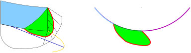 Figure 4
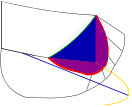 Figure 4
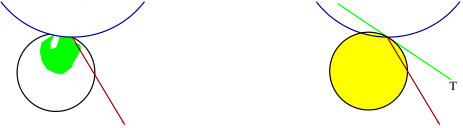 Figure 5
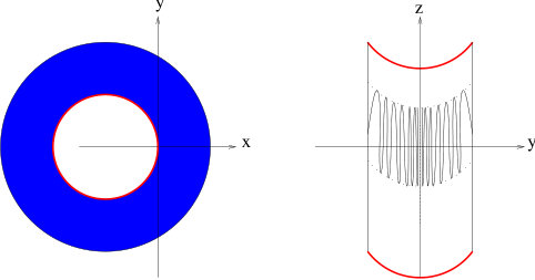 Figure 4