Universal four-dimensional representation of $H \to \gamma \gamma$ at two loops through the Loop-Tree Duality
Felix Driencourt-Mangin, German Rodrigo, German F. R. Sborlini,, William J. Torres Bobadilla

TL;DR
This paper extends the Loop-Tree Duality formalism to two-loop level for the $H\to\gamma\gamma$ process, demonstrating universality, providing a local renormalisation algorithm, and enabling fully four-dimensional numerical computations.
Contribution
It introduces a two-loop extension of the Loop-Tree Duality method with a local renormalisation algorithm, maintaining universality and facilitating 4D numerical calculations.
Findings
Perfect numerical agreement with existing analytic results.
Successful local renormalisation at the integrand level.
Foundation for a 4D framework for higher-order computations.
Abstract
We extend useful properties of the unintegrated dual amplitudes from one- to two-loop level, using the Loop-Tree Duality formalism. In particular, we show that the universality of the functional form -- regardless of the nature of the internal particle -- still holds at this order. We also present an algorithmic way to renormalise two-loop amplitudes, by locally cancelling the ultraviolet singularities at integrand level, thus allowing a full four-dimensional numerical implementation of the method. Our results are compared with analytic expressions already available in the literature, finding a perfect numerical agreement. The success of this computation plays a crucial role for the development of a fully local four-dimensional framework to compute physical observables at Next-to-Next-to Leading order and beyond.
Click any figure to enlarge with its caption.
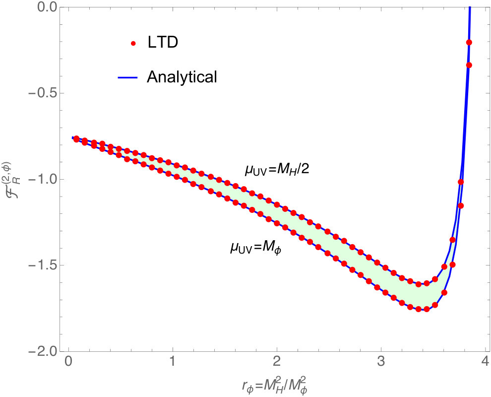 Figure 1
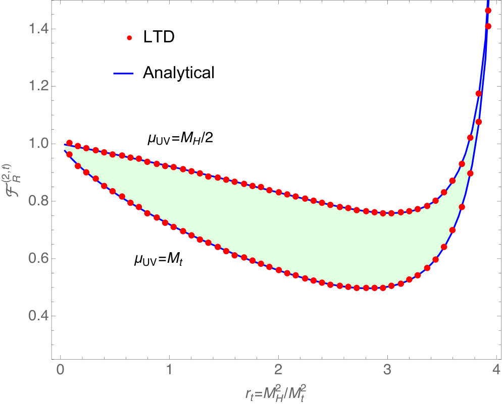 Figure 2
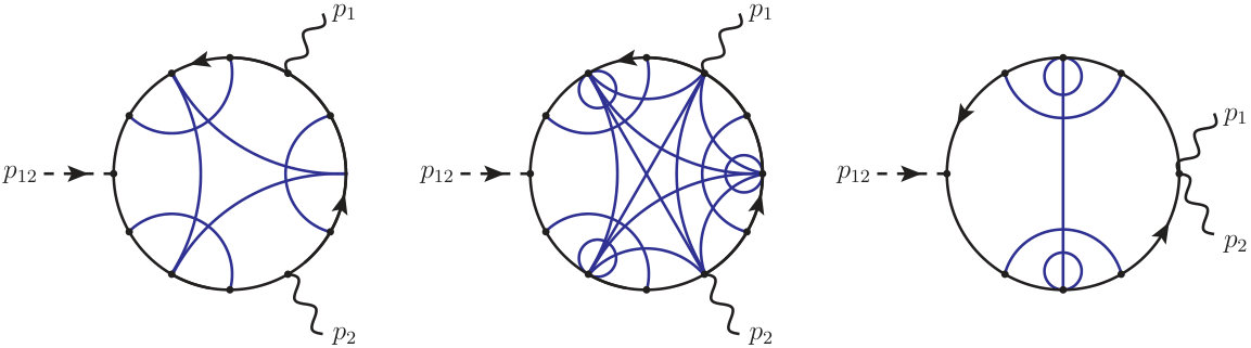 Figure 3
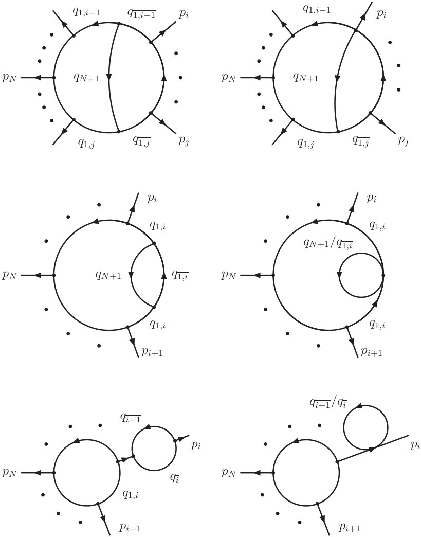 Figure 4
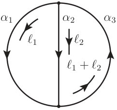 Figure 5
| 1 |
Peer Reviews
No public reviews on file for this paper yet. If you reviewed it on a platform where reviews are public (OpenReview, ICLR, NeurIPS, ICML), you can paste yours below so the community can read it here.
Videos
No videos yet. Explain this paper in a talk, walkthrough, or lecture? Add one.
aainstitutetext: IFIC, Universitat de València-CSIC, Apt. Correus 22085, E-46071 València, Spainbbinstitutetext: Dipartimento di Fisica, Università di Milano and INFN Sezione di Milano, I-20133 Milano, Italyccinstitutetext: International Center for Advanced Studies (ICAS), ECyT-UNSAM, Campus Miguelete, 25 de Mayo y Francia, (1650) Buenos Aires, Argentina.
Universal four-dimensional representation of at two loops through the Loop-Tree Duality
Félix Driencourt-Mangin a
Germán Rodrigo a,b,c
Germán F. R. Sborlini a
and William J. Torres Bobadilla
Abstract
We extend useful properties of the unintegrated dual amplitudes from one- to two-loop level, using the Loop-Tree Duality formalism. In particular, we show that the universality of the functional form – regardless of the nature of the internal particle – still holds at this order. We also present an algorithmic way to renormalise two-loop amplitudes, by locally cancelling the ultraviolet singularities at integrand level, thus allowing a full four-dimensional numerical implementation of the method. Our results are compared with analytic expressions already available in the literature, finding a perfect numerical agreement. The success of this computation plays a crucial role for the development of a fully local four-dimensional framework to compute physical observables at Next-to-Next-to Leading order and beyond.
††preprint: IFIC/18-31 , TIF-UNIMI-2018-6
1 Introduction
The calculation of observables the physics the LHC delivers has nowadays been improved with several techniques to make predictions at the Next-to-Leading order (NLO) accuracy. In general, it is aimed at reducing the scale uncertainties from to , and to even less for some specific processes such as Drell-Yan. In order to provide these observables, we rely our prediction on the calculations of scattering amplitudes through perturbation theory. For the calculation of the latter at NLO, apart from evaluating Feynman integrals, we also need to deal with the evaluation of integrals in the momentum space. At one-loop level, the basis of integrals is known and their evaluation has been implemented in several codes (for instance, in refs. vanHameren:2010cp ; Carrazza:2016gav ). Nevertheless, the evaluation of multi-loop integrals still remains a work in progress Borowka:2015mxa ; Smirnov:2015mct . On top of it, depending on the process under consideration, there may appear infrared (IR) and ultraviolet (UV) singularities that are canceled out by adding real corrections and proper counter-terms.
The two-loop QCD corrections to the decay process have been first evaluated in the heavy-top limit Harlander:2005rq ; Zheng:1990qa ; Djouadi:1990aj ; Dawson:1992cy and with the full top-mass dependence Fleischer:2004vb ; Aglietti:2006tp . The two-loop electroweak corrections have been investigated in refs. Actis:2008ts ; Passarino:2007fp ; Degrassi:2005mc ; Fugel:2004ug . Combining the two-loop QCD and electroweak corrections, it is possible to observe a nearly complete cancellation between these two contributions for GeV Maierhofer:2012vv . At Next-to-Next-to-Leading order (NNLO) the non-singlet Steinhauser:1996wy and singlet QCD contributions Maierhofer:2012vv have been calculated in the heavy top quark limit.
In view of the enormous success of the Standard Model (SM) of particle physics with the detection of the Higgs boson, new directions have been taken to discuss in more details the consequences of this discovery. In particular, from the phenomenological point of view, the background of the experiment has to be removed. Hence, QCD predictions up to the Next-to-Next-to-Next-to-Leading order (N3LO) have been provided in an effective theory Anastasiou:2016cez . Also, it has been shown that the mixed effects of QCD-electroweak contribution to the amplitude are relevant Bonetti:2018ukf .
Nevertheless, hidden mathematical properties of the amplitudes and have been extensively studied in the full theory at Leading order (LO) in ref. Driencourt-Mangin:2017gop , in which, it was showed that these amplitudes exhibited remarkable properties when computed using the Loop-Tree Duality (LTD) theorem Catani:2008xa ; Bierenbaum:2010cy ; Bierenbaum:2012th . The dual contributions we have obtained for different internal particles – charged electroweak gauge bosons, massive fermions and charged scalars – featured the very same functional forms, and could be written in a universal way using scalar parameters depending only on the space-time dimension (), and the mass of the particles involved in the process. We also obtained a pure four-dimensional () representation of the renormalised amplitude and recovered the well-known results found in the literature Wilczek:1977zn ; Georgi:1977gs ; Rizzo:1979mf ; Ellis:1975ap ; Ioffe:1976sd ; Shifman:1979eb .
In this manuscript we push the computation further by considering the process at two-loop level, and show that the above-mentioned properties are still present. To this end, we make use of the LTD theorem, which converts loop integrals into phase-space ones. In order to provide the renormalised amplitude, we perform a local UV renormalisation that leads to a finite integrand in four space-time dimensions. This algorithm is based on the refinement of the expansion around the UV propagator Becker:2010ng ; Sborlini:2016gbr ; Sborlini:2016hat to account for the different singular behaviours of the internal loop momenta in the UV region. Furthermore, since this amplitude is IR safe, we can directly treat the virtual integrand in four dimensions. We remark that the calculation of this amplitude is the first two-loop application to a physical process done through LTD, and it is computed below the mass threshold limit in the renormalisation scheme. We note that for individual diagrams, unphysical threshold singularities appear but they cancel among themselves when the full amplitude is considered.
In the same spirit of the universality that these amplitudes exhibit at LO, we consider as internal particles charged scalars and top quarks. While we only consider QED corrections, they can be straightforwardly promoted to QCD ones by replacing the couplings accordingly. We compare our results with known results Fleischer:2004vb ; Aglietti:2006tp finding full agreement.
With this paper we verify that the LTD approach holds also at multi-loop level and, therefore, NkLO predictions involving virtual amplitudes can be achieved by means of the former. Additionally, we remark that the traditional approach based on the use of integration-by-parts identities Chetyrkin:1981qh ; Laporta:2001dd is not needed to evaluate the actual amplitude. In fact, we overcome the calculation of the latter making our procedure much lighter as we shall describe here.
The paper is organised as follows. In section 2, we recall the basics of the LTD formalism, at one- and two-loop level. We introduce there the notations used in this paper, and provide the master formula for obtaining the dual representation of a two-loop Feynman integral. In section 3, we sketch the algorithm to algebraically reduce the integrand-level expressions of two-loop dual amplitudes, and rewrite every scalar product involved in terms of denominators. We provide the tensor structure of the amplitude in section 4, and briefly recall the one-loop result obtained in ref. Driencourt-Mangin:2017gop . Then, in section 5, we collect and write the universal coefficients involved in the universal structure of the two-loop dual expressions. We discuss in section 6 the cancellations of unphysical threshold singularities that appear among the dual contributions, and we explicitly show how they occur. In section 7, we discuss an algorithmic approach to locally renormalise two-loop amplitudes within the LTD formalism. In particular, we focus on the determination of the scheme-fixing parameters in the scheme. In section 8, we present our numerical results and show there is a complete agreement with the analytical expressions. We draw our conclusions and discuss future directions of this work in section 9.
Algebraic manipulations have been carried out by using an in-house implementation of LTD which is based on the Mathematica packages FeynArts Hahn:2000kx and FeynCalc Mertig:1990an ; Shtabovenko:2016sxi .
2 The Loop-Tree Duality at two loops
The Loop-Tree Duality (LTD) theorem Catani:2008xa ; Bierenbaum:2010cy ; Bierenbaum:2012th transforms any loop integral or loop scattering amplitude into a sum of tree-level like objects that are constructed by setting on shell a number of internal loop propagators equal to the number of loops. Explicitly, LTD is realised by modifying the prescription of the Feynman propagators that remain off shell
[TABLE]
with , and an arbitrary future-like vector. The most convenient choice is , which is equivalent to integrate out the loop energy components of the loop momenta through the Cauchy residue theorem. The left-over integration is then restricted to the Euclidean space of the loop three-momenta. The dual prescription can hence be either for some dual propagators or for the others, since indeed only the sign matters. In fact, this prescription encodes in a compact and elegant way the contribution of the multiple cuts that are introduced by the Feynman tree theorem Feynman:1963ax . The on-shell condition is given by , and determines that the loop integration is restricted to the positive energy modes, , of the on-shell hyperboloids (light-cones for massless particles) of the internal propagators. We also introduce the short-hand notation for the loop integration measure in dimensions,
[TABLE]
where is an arbitrary mass scale to compensate the extra dimensions generated by -dimensional integration measure. In the following, we use according to the convention of ref. Gnendiger:2017pys .
In order to generalise LTD to higher orders, we introduce the following functions Bierenbaum:2010cy
[TABLE]
where labels all the propagators, Feynman or dual, of a given subset. An interesting identity fulfilled by these functions is the following
[TABLE]
involving the union of two subsets and . These are all the ingredients necessary to iteratively extend LTD to multi-loop level. For example, at one loop, the Feynman and the dual representations of a -leg scattering amplitude are
[TABLE]
respectively, where is the numerator that depends on the loop momentum and the four-momenta of the external partons . In the absence of multiple powers of the Feynman propagators, the numerator is not altered by the application of the Cauchy theorem. However, the calculation of the residues of multiple poles to obtain the corresponding LTD representation requires the participation of the numerator. This is represented in eq. (5) by the symbol .
At two-loop level, all the internal propagators can be classified into three different subsets (e.g. those depending on , and their sum , as shown in figure 1). Starting from the Feynman representation of a two-loop scattering amplitude
[TABLE]
by applying LTD to one of the loops (eq. (5)), we obtain in a first step:
[TABLE]
Before applying LTD to the second loop, it is necessary to use eq. (4) to express the dual function in a suitable form. The identity in eq. (4) splits the dual integrand into a first term that contains two dual functions – and therefore two internal lines on shell – and two more terms with a single dual function and Feynman propagators involving the other two sets of propagators, to which we can recursively apply LTD. The final dual representation of the two-loop amplitude in eq. (6) is
[TABLE]
In eq. (8), it is necessary to take into account that the momentum flow in the loop formed by the union of and occurs in opposite directions. Therefore, it is compulsory to change the direction of the momentum flow in one of the two sets. This is represented by adding a sign in front of e.g. , explicitly we have
[TABLE]
Changing the momentum flow is equivalent to select the negative energy modes. For the internal momenta in the set , this means
[TABLE]
The dual representation gets its simplest form if the Feynman representation contains only single powers of the Feynman propagators. This restriction cannot be avoided anymore at two-loops where, for example, self-energy insertions in internal lines lead automatically to double powers of one propagator. However, all the double poles can be included with a clever labelling of the internal momenta in the set , exclusively, which is not integrated in the first instance. Therefore, we have assumed that the numerator in eq. (7) is not affected by the application of LTD. The final dual representation in eq. (8) depends, in general, on the explicit form of the numerator. Again, this is represented by the symbol .
The number of independent double cuts in eq. (8) per Feynman diagram is
[TABLE]
where counts the number of propagators in each set. Therefore, it is convenient to have as the set with the smallest number of propagators. For planar diagrams, the set contains one single propagator.
It is interesting to note that although the integration over the loop three-momenta is unrestricted, after analysing the singular behaviour of the loop integrand one realises that thanks to a partial cancellation of singularities among different dual components, all the physical threshold and IR singularities remain confined to a compact region of the loop three-momentum Buchta:2014dfa ; Buchta:2015wna . This relevant fact allows to construct mappings between the virtual and real kinematics, which are based on the factorisation properties of QCD, to implement the summation over degenerate soft and collinear states for physical observables in the Four-Dimensional Unsubtraction (FDU) formalism Hernandez-Pinto:2015ysa ; Sborlini:2016gbr ; Sborlini:2016hat . This framework, however, is not going to be needed in the following. This is because, as we shall see in section 6 where we analyse the cancellation of singularities at two loops, no infrared singularities remain when considering the full amplitude.
3 Algebraic reduction of two-loop dual amplitudes
In order to make the two-loop expressions more compact, we perform an algebraic reduction of the dual amplitudes to dual integrals that involve both positive and negative powers of dual propagator denominators. We analyse only the case of planar diagrams that are those that appear in the practical example that we present.
Let us first consider scattering amplitude with external legs and ordered external momenta. At one-loop, we have different propagators and independent scalar products (indeed, because of momentum conservation, , with the loop four-momentum). In the Feynman representation, the propagators are quadratic in , while in LTD the dual propagators are linear. In both formalisms, however, it is possible to write numerators in terms of propagators diagram by diagram.
Now, we consider the set of two-loop planar Feynman diagrams constructed from the ordered one-loop seed diagram – that is, all the two-loop diagrams that have one loop line involving one single propagator (see figure 2 for the assignment of momenta). These planar two-loop Feynman diagrams can be constructed from the sets of propagators
[TABLE]
with , , and . These propagators are constructed by attaching in all possible ways while keeping the same ordering of the external momenta in the loop formed by the other two loop lines and . This sums to possible propagators. If there are only three-point interactions, each Feynman diagram contains propagators from these sets. If there are four-point interaction vertices, each individual Feynman diagram contains only propagators.
Because of momentum conservation, there are independent scalar products that are
[TABLE]
In LTD at two loops, two internal particles are set on shell, which means that only dual propagators remain for a given double cut. Moreover, dual propagators are linear in each of the loop momenta, and the dual numerators do not involve squared loop-momenta. Therefore, for each double cut, and considering all the Feynman diagrams with the same ordering of the external particles, it is possible to rewrite all the scalar products involved (and thus the numerators) in terms of dual propagators, and this in a unique way. Due to the assignment of the loop momenta, all the required irreducible scalar products (ISP) are automatically introduced. This is because the set of Feynman diagrams contains all the necessary propagators to perform the complete algebraic reduction.
The algebraic reduction of a planar two-loop dual amplitude with external legs, and at most squared propagators in one single loop line, leads to
[TABLE]
with111At this point is is not necessary to make the distinction, because… or , and
[TABLE]
The scalar coefficients depend only on the external momenta, and are not necessarily independent. Our purpose is to rearrange the expressions for the dual amplitudes in order to obtain the minimal set of independent coefficients . Another relevant issue to obtain the most compact integrand expressions is to label the internal momenta in the most symmetric way. In figure 2, we show the assignments that we use in the most general case for planar two-loop diagrams. Computer algebra programs for the automatic generation of two-loop amplitudes, like FeynArts Hahn:2000kx , might use a different criteria which require a relabelling of the internal propagators to achieve the most suitable assignment. In the next sections, we shall illustrate the full procedure with the benchmark amplitude .
4 Tensor projection and at one loop
The scattering amplitude describing the Higgs boson decay to two photons is given by
[TABLE]
with the electromagnetic coupling, (respectively ) the electric charge (respectively the number of colours) of the virtual particle , and the polarisations vectors of the external photons. Here, we assume that the two photons are coupled to the same flavour. We are interested in the QED corrections at two-loop level with . The tensor amplitude fulfils the perturbative expansion
[TABLE]
where is the one-loop amplitude, and is the two-loop QED correction. The tensor amplitudes can be decomposed through Lorentz and gauge invariance as
[TABLE]
in terms of the tensor basis
[TABLE]
The tensor structure may appear for the first time at two-loop, because of the potential presence of a , but its interference with the one-loop amplitude vanishes. As in ref. Driencourt-Mangin:2017gop , we use the projectors
[TABLE]
to extract the scalar amplitudes and . There is no need to compute , for , as they vanish after contracting with the polarisation vectors, and therefore do not contribute to the scattering amplitude for on-shell photons. Moreover, because of gauge invariance, is expected to vanish after integration, which leaves as the only relevant physical term. It is still interesting to consider and get integrand expressions for , though, as it can be used to simplify expressions.
The dual representations of the one-loop amplitudes and were calculated in ref. Driencourt-Mangin:2017gop in terms of the global factor and scalar coefficients , which have the form with and . For the three different virtual particles that we considered, these coefficients are given by
[TABLE]
The vanishing one-loop amplitude is given by
[TABLE]
where , with . The on-shell loop energies are given by
[TABLE]
As stated above, we know that after integration due to gauge invariance. Therefore, we can use this feature to simplify the expression for . Already at one loop (), we showed that the following transformation Driencourt-Mangin:2017gop
[TABLE]
with , and
[TABLE]
reduces the number of necessary independent scalar coefficients to describe from three to two. Notice that while they are labelled differently because they do not have the same integrand-level expressions, we have after integration222Note that integrates to 0 in dimensions, whereas in four space-time dimensions it is only the case after local renormalisation.. For the complete expression of the amplitude, we obtain
[TABLE]
It is remarkable to note that the dependence on the nature of the internal particle appears in eq. (22) and eq. (26) only through the scalar coefficients , defined in eq. (21).
Although is UV finite, because there is no direct coupling of the Higgs boson to photons at tree level, its integrand expression still exhibits a local UV behaviour. For that reason, we defined in ref. Driencourt-Mangin:2017gop the UV counter-term
[TABLE]
with . The UV counter-term in eq. (27) integrates to zero in -dimensions, though, it is used to cancel the local UV behaviour of eq. (26) in such a way that the locally renormalised one-loop amplitude can be obtained without altering the dimensions of the space-time
[TABLE]
5 Dual amplitude for at two loops
At two-loop level, there are 12 Feynman diagrams contributing to the scattering amplitude with internal top quarks. For internal charged scalars, there are 37 Feynman diagrams. The corresponding two-loop diagrams are drawn in figure 3 where all those that share the same global topology are superimposed in the so-called mandala diagrams. In this paper, we only consider QED corrections, and therefore photons as the extra internal particle, and do not take into account “mixed” diagrams where different massive particles may appear. In the traditional approach, massless snail diagrams are usually ignored, since they integrate to zero. However, within our approach, we need them to preserve the universal structure of the integrands.
All the diagrams are planar and can be constructed from the following internal momenta:
[TABLE]
Only (and ) is massless (it labels the photon), while all the other internal momenta have mass .
If the Higgs boson is on shell, the loop amplitude is below threshold and is therefore purely real. In that kinematical regime the dual prescriptions become irrelevant, and the dual functions fulfil the identity
[TABLE]
Hence, the LTD representation in eq. (8) adopts the simpler form
[TABLE]
Following the algebraic reduction defined in section 3,
[TABLE]
with ,
[TABLE]
For a given dual or Feynman propagator, we have defined the dimensionless denominator . For example, in terms of these dimensionless denominators, the one-loop amplitude in eq. (26) takes the form
[TABLE]
with
[TABLE]
From now on, we use a different global factor depending on whether the expressions it multiplies has been algebraically reduced or not. The usual will be used for unreduced expressions, and for reduced ones.
5.1 The two-loop amplitude
The two-loop amplitude is obtained by projecting using the projector defined in eq. (20), namely . Due to gauge invariance, it has to vanish after integration. Still, it is interesting to obtain an explicit expression because it establishes a useful integrand relation that can be used afterwards. Remarkably, it can be written in a very compact form for :
[TABLE]
where
[TABLE]
and where the coefficients and can be found in eqs. (5.2) and (5.2). Notice there is a difference in mass dimensions between and . This is due to the presence of the second loop measure and the additional , whose product has dimension of mass squared. The following contribution
[TABLE]
vanishes irrespective of the rest of the expression for because the following subintegrals, with , are equivalent
[TABLE]
Consequently, the sum over integrals in eq. (38) vanishes.
5.2 The two-loop amplitude
In this section, we apply the same transformation in eq. (24) at two-loop () to simplify the expressions for the amplitude . Then, and as explained in section 3, we perform an algebraic reduction to express the dual representation in the form eq. (32) and extract the scalar coefficients . As very few of them are indeed independent, they are simply relabeled as . We obtain very compact expressions for all the double cuts of the LTD representation. The full expressions for the unrenormalised amplitude are collected in appendix A. As for the one-loop case, the same expressions are valid regardless of the virtual particle circulating in the loop as a function of the flavour-dependent coefficients .
For the top quark and the scalar, the two independent coefficients that appeared at one loop are (see eq. (21))
[TABLE]
At two loops, they are still present, along with the following extra coefficients:
[TABLE]
Notice that these coefficients can be highly simplified in the particular case , motivating further the study of a full four-dimensional representation of this process at two-loop level.
6 Cancellation of integrand singularities at two loops
In addition to be infrared safe, the scattering amplitude for is purely real if the Higgs boson is on shell. It is therefore completely free of soft and physical threshold singularities. Still, some of the dual propagators might go on shell inside the integration domain, leading to singularities of the integrand. As we demonstrated in refs. Buchta:2014dfa ; Buchta:2015wna at one-loop level, one of the advantages of LTD is the partial cancellation of potential singularities of the integrand. In this section, we extend the analysis of the integrand singularities of at two-loop level.
If a dual propagator becomes on shell where both internal momenta and belong to the same loop line , then the corresponding singular behaviour is equivalent to the one-loop case. For example, consider the dual propagator . A physical threshold (forward-backward singularity333A forward-backward singularity in the loop momentum space arises in the intersection of the forward on-shell hyperboloid or positive energy mode of one propagator with the backward on-shell hyperboloid or negative energy mode of another propagator.) occurs if (see ref. Buchta:2014dfa )
[TABLE]
with and . Therefore, but for . An integrand singularity (forward-forward singularity) occurs if
[TABLE]
This would be the case of, e.g., because , but this integrand singularity cancels in the sum of the two dual contributions involving and . The analysis can be extended easily to the other dual cuts, and similar conclusions are found.
Now, we consider the genuine two-loop case where a dual propagator becomes on shell in the double cut of two propagators that do not belong to the same loop line. For the rest of this section, we consider
[TABLE]
We study study the quantity444A rigorous analysis would require to consider either or . For the sake of simplicity, denotes the dual propagator obtained by ignoring the imaginary dual prescription, with both and on shell. This simplification is valid because we are dealing with a real scattering amplitude.
[TABLE]
where indicates that we reverse the momentum flow of , as explained in section 2, namely
[TABLE]
We therefore have
[TABLE]
where
[TABLE]
only depends on external momenta. The quantity becomes singular in the limits summarised by the condition , with
[TABLE]
Accorded to eq. (49), only four independent solutions have to be considered, namely , , and . For two of these limits, there is a perfect cancellation of the integrand singularities, as indeed
[TABLE]
while for the remaining two limits,
[TABLE]
Although these singularities remain in the general case, it is possible to show that (resp. ) can only cancel if, in the particular case where and ,
[TABLE]
Because of the fact does not depend on the loop momenta, the highest possible value of is , reached for instance when considering . This means the second condition of eq. (54) reduces to
[TABLE]
which is not fulfilled if, as stated above, the Higgs boson is assumed to be on shell, i.e. .
Now, we consider the possibility to encounter soft singularities as one of the internal particles is massless. The integrand becomes soft in the loop momentum if . In that case, the analysis of the singular behaviour is very similar to the one-loop case. We should solve the condition
[TABLE]
in . If the three propagators are attached to the same vertex, then and . In that case and can vanish, then enhancing the integrand singularity in , but the overall singularity cancels between dual contributions. The other solution, with , is not possible because . If the three propagators do not interact in the same vertex, then . This configuration includes the cases where and belong to the same or to different loop lines. There are solutions to eq. (56), but again either they cancel among dual contributions or eq. (44) is not fulfilled. In all the cases, the soft singularities of the integrand in do not translate into soft singularities of the amplitude because of the integration measure.
7 Algorithmic approach to two-loop local UV renormalisation
Let us consider a generic unrenormalised two-loop amplitude , written as
[TABLE]
which we will assume to be completely free of any infrared singularity. Thus, only UV singularities may appear when either or both of and go to infinity. The local two-loop UV counter-terms are built recursively by first fixing one of the two loop momenta, say , and expanding the integrand up to logarithmic order around the UV propagator Becker:2010ng
[TABLE]
where the arbitrary scale represents the renormalisation scale, and . For simplicity, we take . The quantity
[TABLE]
where denotes the two-loop amplitude in the limit , is not necessarily UV finite when both loop momenta are simultaneously large. It is necessary to subtract also the double UV behaviour of eq. (59). With this contribution, which is represented by , the final renormalised amplitude reads
[TABLE]
and is UV safe in all the limits. As an example, we consider
[TABLE]
This integrand produces a UV singularity when , but it is superficially regular in , meaning . Computing the remaining counter-term gives
[TABLE]
which effectively removes the UV behaviour in , but at the same time also introduces a singularity in . It is therefore necessary to introduce the additional counter-term to fix the UV behaviour when both loop momenta go to infinity. This is done by expanding eq. (59) for very high values of and , while never neglecting one compared to the other. In this example, we get
[TABLE]
Then, the renormalised amplitude, as defined in eq. (60), is finite in the UV. It is still necessary, though, to introduce subleading contributions to fix the renormalisation scheme. This is better explained in the following for the two-loop amplitude.
With the labelling of the internal momenta that we have adopted for the amplitude, it is more convenient to express the UV behaviour at two loops in terms of and , with . Explicitly, the single and double UV behaviours are implemented by making use of the following transformations
[TABLE]
then expanding for and truncating the corresponding series in up to logarithmic degree. This last operation is represented by the function . In particular, the UV counter-terms are defined as
[TABLE]
where is the unintegrated one-loop amplitude written in terms of ( or ) with , and where and are scalar coefficients used to fix the renormalisation scheme. Note that the integrals they multiply integrate to finite quantities. The factor 4 appearing in the second line of eq. (66) is arbitrary and has been introduced to conveniently rescale .
7.1 Higgs boson vertex renormalisation
In the Feynman gauge, the one-loop QED correction to the Higgs boson vertex exhibits the UV behaviour
[TABLE]
where and are the tree-level vertex interactions, and . The coefficients are subleading and are necessary to fix the renormalisation scheme. The values of these coefficients in the renormalisation scheme555We distinguish from the usual scheme factor or as used in ref. Bolzoni:2010bt . At NLO all these definitions lead to the same expressions. At NNLO, they lead to slightly different bookkeeping of the IR and UV poles at intermediate steps, but physical cross-sections of infrared safe observables are the same. are summarised in table 1, and they are related to the coefficient of the integrated vertex counter-term through
[TABLE]
From the expression of the vertex counter-term in eq. (67) we can construct the UV counter-term of the two-loop scattering amplitude in the limit with fixed. It reads
[TABLE]
where is the unrenormalised one-loop amplitude in eq. (26). Note that is locally divergent and should be renormalised as well in eq. (69). However, by definition, we want to exactly cancel the singularities arising when . Putting instead of in eq. (69) would therefore alter the UV behaviour of the single counter-term and not properly remove the corresponding infinities. It is only when considering the double UV counter-term (section 7.4) that the one-loop amplitude implicitly gets renormalised.
The corresponding dual representation is
[TABLE]
where . Since the diagrams (2 for the top quark, 3 for the charged scalar) that contribute to the Higgs vertex correction are the only ones that are divergent when , we directly have .
7.2 Photon vertex renormalisation
The one-loop correction to the photon interaction vertex to top quarks in the UV is given in the Feynman gauge by
[TABLE]
with
[TABLE]
In eq. (71), the term proportional to integrates to zero in space-time dimensions. Similarly to eq. (68), the coefficient of the integrated vertex counter-term is given by
[TABLE]
Although the integrated UV vertex correction is proportional to the tree-level vertex , thanks to the replacement , we cannot use this replacement in the unintegrated form because it would alter the local UV behaviour. We must keep the full expression in eq. (71), including especially the term proportional to , to construct the local UV counter-term of the two-loop scattering amplitude.
For charged scalars as internal particles, we need to consider both the three-point and the four-point interaction vertices. For the three-point vertex there are three contributing diagrams, and the corresponding counter-term reads
[TABLE]
where
[TABLE]
with and , where and are the outgoing and incoming internal momenta, respectively. For example, and for the vertex correction with emission of a photon with momentum in the lower corner of the two-loop Feynman diagram.
For the four-point interaction vertex, there are nine contributing diagrams666Note that these diagrams include the ones contributing to the Higgs vertex correction. However, the singular regime considered here is different since we study the limit ., and we have
[TABLE]
where
[TABLE]
with . Remarkably, the coefficient is the same as for the three-point interaction vertex. Again, in eq. (74) and eq. (76), we cannot apply the replacement at integrand level even though the terms in eq. (74) and in eq. (76) integrate to zero. Also notice that it was not necessary to introduce subleading terms for the scalar vertices because the finite part of the corresponding integrated counter-term is already 0.
The integrated counter-term reads
[TABLE]
where is the sum of the two one-loop amplitudes involving triangle diagrams and is the one-loop bubble amplitude (which appears only for the charged scalar). The relative factors 2 in eq. (78) comes from the fact there are two three-point vertices to renormalise for each contributing diagram.
The corresponding dual representations are
[TABLE]
where .
7.3 Self-energies renormalisation
With our labelling of the momenta the self-energy insertions are defined in terms of the internal momenta and , with . Explicitly, in the Feynman gauge we have (notice the relative sign in with respect to Sborlini:2016hat because of the fact the momentum flows in the opposite direction)
[TABLE]
The UV expansion of eq. (82) reads
[TABLE]
with
[TABLE]
where the coefficients are subleading contributions to be fixed through the renormalisation scheme. It is remarkable that it has been possible to write the quark self-energy in terms of the same coefficients that appear in the Higgs boson and photon vertices. Notice that the expression in eq. (83) is simpler than the corresponding expression provided in ref.Sborlini:2016hat and only differs at , which does not have any consequence at the considered order.
The scalar self-energy corrections, which also include the snail diagrams, is written
[TABLE]
where , or, equivalently, . One possibility would be to subtract the contribution which is proportional to before expanding in the UV, which would be equivalent to subtract a zero (actually this would not only work for the term generated by the snail diagrams, but also for any term that exclusively contains propagators depending only on ). However, it would modify only the double cuts . The UV expansion of eq. (85) reads
[TABLE]
with
[TABLE]
[TABLE]
The terms and integrate to zero independently in dimensions. In the latter, i.e. eq. (88), it was necessary to include a subleading contribution, proportional to . We will not provide the integrated and dual expressions for because they are quite heavy.
Finally, the counter-term is simply obtained by considering the photon vertex and self-energy contributions together, namely
[TABLE]
7.4 The double UV counter-term
While it is entirely possible to compute by directly taking the sum of all contributions, it is more interesting to consider well-chosen subsets of diagrams – it also lightens intermediate expressions. For the top as the internal particle, it is logical to consider all the contributions to the Higgs boson vertex corrections, all the contributions to the photon vertex corrections and all the contributions to the self-energy corrections, as there is no ambiguity or cross-contributions for the process at two-loop. They will be written , , , and account for 2, 4 and 6 diagrams, respectively. For the charged scalar as an internal particle, there is a subtlety. The three diagrams that contribute to the Higgs vertex correction also contribute to the vertex correction. For this reason, if we want to split , we have to consider both corrections together. For the photon and self-energy corrections, though, there is no ambiguity whatsoever. Thus, we define , , , that account for 9, 12 and 16 diagrams, respectively.
According to eq. (66), the unintegrated double UV counter-terms have the form
[TABLE]
where
[TABLE]
and with being positive integers. Note that even though should be expected to also depend on the external momenta and , it is a remarkable feature that, thanks to welcome cancellations, it does not when considering the sum of all contributing diagrams. The expression in eq. (90) is therefore free of irreducible scalar products and can very easily be reduced through integrations by parts to the form
[TABLE]
where
[TABLE]
with
[TABLE]
where is the Clausen function of order 2, is the sunrise scalar integral with missing external momenta and all the internal masses equal, and
[TABLE]
is the massive tadpole. Because of the presence of the double pole inside eq. (93), it is, in the general case, necessary to keep track of the different normalisations as choosing one over another could lead to a shift in the finite part. As we are working in the scheme, we should rather factorise the usual , but doing so, a global factor equal to would appear. We will see that in the end considering one normalisation over the other does not introduce any mismatch, so we chose to keep for simplicity.
These two master integrals (MI) are the only ones needed to evaluate and fix the subleading terms . Note that in eq. (92), the dependence in is implicitly included in .
The unintegrated double UV counter-term for the diagrams with loop corrections in the Higgs boson vertex and internal top quarks reads
[TABLE]
and gives
[TABLE]
where the parameter has been replaced by its value, given in table 1. After integration, we have
[TABLE]
The unintegrated expressions for the double UV counter-term for the photon and self-energy corrections are a bit heavy, so we will only provide the MI coefficients. For the photon vertex corrections, they read
[TABLE]
while for the self-energy corrections, they read
[TABLE]
where once again we replaced and by their value. Integrating the counter-terms gives
[TABLE]
and
[TABLE]
leading to
[TABLE]
where we used .
For the scalar, the unintegrated double UV counter-term for the Higgs and corrections read
[TABLE]
which after IBP reduction gives
[TABLE]
We obtain
[TABLE]
As for the top, the unintegrated expressions for and are a bit heavy. Their corresponding MI coefficients are
[TABLE]
and
[TABLE]
After integration, we find
[TABLE]
and
[TABLE]
leading to
[TABLE]
The coefficients can now be very easily be adjusted to obtain the desired part. Their value in the scheme are listed in table 2.
It is remarkable that for both particles, the full double UV counter-terms does not exhibit any -poles, justifying in the mean time that using instead of does not introduce any discrepancy in the final result. While for the top quark each intermediate double UV counter-terms are all finite, for the charged scalar the cancellation of divergences only occurs when taking into account the sum of all 37 diagrams. This is due to the fact there are more subtle interplays between different contributing topologies, because of the more complex gauge structure. In both cases, the absence of divergences after integration means that in the traditional approach, these double UV counter-terms should not be needed. In our formalism however, they are essential in order to cancel local divergent behaviours appearing inside the amplitude and the single UV counter-terms. Note also that the unintegrated counter-terms exhibit terms proportional to that vanish when taking the four-dimensional limit at integrand level, even though they still lead to finite parts when keeping the dependence, because they multiply quantities that exhibit -poles. This means that while the counter-terms are finite, they will not lead to the same result if computed in or 4 dimensions. It is only when considering the renormalised amplitude that we have a strict and rigorous commutativity between integrating and taking the limit . The same happens at one-loop level Driencourt-Mangin:2017gop , where the counter-term would not be needed (it integrates to 0 in the ) in dimensions. One can wonder if this property holds at three-loop order and beyond, if it is exclusive to the process and why, and if there is an underlying reason behind it.
8 Numerical integration
The renormalised unintegrated amplitude is completely free of local UV (and IR) singularities and can safely be evaluated in four dimensions. In the centre-of-mass frame of the decaying Higgs boson, we parametrise the three-momenta as
[TABLE]
Note that we can assume , for instance, to belong to the plane, as there is a global rotational symmetry; this means we can trivially perform the integration over one azimuthal angle – leading to a factor – and set to 0. Furthermore, it is better to use instead of as integration variable, because of the way the UV counter-terms have been defined. We therefore integrate over the two three-momenta
[TABLE]
which leads to five integration variables, namely , and . In addition, the usual compactification of the integration domain is performed, where the domains of and are mapped from onto to , thanks to the change of variables
[TABLE]
with , and . This increases the stability of the numerical integration for very high energies, because it restricts the local cancellation of UV singularities to a compact region. The integration measure, after applying this change of variables and in four dimensions, reads
[TABLE]
Directly writing all the dual cuts explicitly in terms of the integration variables would not lead to a reasonable computational time, as the integration would be too heavy numerically speaking. Moreover, it would be far from being optimal, since many identical terms would have to be evaluated more than once. Instead, we take advantage of the fact it was possible to write all dual cuts in terms of the reduced denominators , as explained in section 3 and shown in appendix A. The first step, which only needs to be done once, is to express all the reduced denominators in terms of the 5 integration variables, and this for each dual cut777Recall that the expression of a given differs from dual cut to dual cut.. We can then compute their numerical values for a given point in the integration domain, which allows us to quickly evaluate the integrand at this very point by appropriately replacing each . Thus, regardless of the complexity of a given integrand, only a limited amount of objects have to be numerically evaluated. Although quite simple to implement, this strategy helped decreasing the integration time by more than one order of magnitude. To perform the actual integration, we used the in-built Mathematica function NIntegrate. Our results are shown in figure 4, where they are compared with the analytical results given in appendix B. The integration time is of a few minutes for each point. The biggest source of numerical error comes from the cancellation, between the amplitude and the double UV counter-term, of the non-decoupling term going as . For for example, the part being removed from the amplitude by the counter-term is two orders of magnitude higher than the actual result, effectively multiplying the relative numerical error by a factor 100, roughly. Note that this error is twice as big for the top quark as for the charged scalar, because of the relative factor -2 between their respective terms. Nevertheless, the agreement with the analytical result is excellent for all values of the internal and renormalisation masses considered. Numerical instabilities may however appear when considering very close to 4 (or equivalently very close to ), as we approach the mass threshold. Beyond this limit (), contour deformation would be needed. Within the LTD formalism, numerical implementations of contour deformation have already been successfully implemented in Buchta:2015wna .
9 Conclusion
In this paper, we have studied a purely four-dimensional representation of the renormalised Higgs boson decay amplitudes at two-loop order, so that it can directly be evaluated numerically. For this purpose, we have applied the Loop-Tree Duality (LTD) theorem to the process, where internal particles are charged scalars and fermions. Working at the two-loop level within this formalism involves performing double-cuts and several algebraic manipulations of the expressions. This has been done through a fully automatised Mathematica code which can be adapted to deal with any two-loop scattering amplitude.
Once the full sets of double-cuts were generated, we have taken advantage of the previously known one-loop results Driencourt-Mangin:2017gop , in order to infer the universal integrand-level structure of the two-loop expressions. Surprisingly, we have found many similarities between both cases, which has allowed us to write the full two-loop amplitude at integrand level using the same functional forms independently of the nature of the particles circulating inside the loop. As in the one-loop case, the explicit process dependence is codified inside specific scalar coefficients.
We have kept the dependence in all intermediate steps, although a noticeable simplification of the universal coefficients takes place in the limit . We have studied the singular structure of the two-loop amplitudes to understand how to achieve a purely four-dimensional representation of the finite parts. In the first place, we have studied the cancellation of spurious threshold singularities that appear as a consequence of splitting the different cuts. When considering below the physical threshold, the amplitude is guaranteed to be infrared safe as well as free of any physical threshold singularity. In fact, we have managed to prove that all the spurious singularities vanish in this configuration after putting together all possible double cuts.
Then, we have developed a fully local framework to remove ultraviolet singularities. We have implemented an algorithmic approach to renormalise, at integrand level, the two-loop amplitudes. It is based on the refinement of the expansion around the UV propagator strategy Driencourt-Mangin:2017gop ; Sborlini:2016gbr ; Sborlini:2016hat , including an iteration to remove all the possible UV divergences. A careful study of the UV structure of vertices and self-energies has been performed, which allowed to impose constraints on the finite remainder containing the specific renormalisation scheme dependence. Furthermore, we have also shown that the UV scale we used in the derivation of the local counter-terms corresponds to the renormalisation scale used in the traditional approach. These last two points allowed to build the required counter-terms at integrand level to reproduce the results.
Finally, we have proceeded to combine the universal dual representations of the amplitudes together with the local UV counter-terms, achieving a fully renormalised integrand in four space-time dimensions. This has allowed a purely numerical implementation which fully agrees with the available results in the literature. On top of that, intermediate checks with the scalar sunrise diagram were implemented, in order to test the reliability of the codes.
The results presented in this paper constitutes a major advance into the extension of the Four-Dimensional Unsubtraction (FDU) formalism Sborlini:2016gbr ; Sborlini:2016hat to NNLO accuracy, paving the way for a more efficient and purely numerical implementation of currently relevant physical processes.
Acknowledgements
This work is supported by the Spanish Government (Agencia Estatal de Investigación) and ERDF funds from European Commission (Grants No. FPA2017-84445-P and SEV-2014-0398), by Generalitat Valenciana (Grant No. PROMETEO/2017/053) and by Consejo Superior de Investigaciones Científicas (Grant No. PIE-201750E021). FDM acknowledges support from Generalitat Valenciana (GRISOLIA/2015/035) and GFRS from Fondazione Cariplo under the Grant No. 2015-0761. WJT acknowledges support from the Spanish government (FJCI-2017-32128). Also, FDM and GFRS were supported by a STSM Grant from the COST Action CA16201 PARTICLEFACE.
Appendix A Unrenormalised two-loop dual amplitudes for
In this appendix, we collect the explicit expressions for the unrenormalised two-loop dual amplitudes for . The subindices take the values and , with . The functions and have been defined in eq. (LABEL:eq:FG). Here, we introduce the auxiliary function
[TABLE]
For example
[TABLE]
[TABLE]
[TABLE]
with (recall that ). It is very important to note that the permutation inside the following expressions have to be applied on the parameters of , instead of the expression of itself after derivation, as the symmetry is not any more explicit.
A.1 Double cuts from
This is the only set with direct snail contributions for scalars, the only terms that do not depend on are those proportional to and . This subset generates 4 different double cuts that are obtained from the following expressions:
[TABLE]
and
[TABLE]
A.2 Double cuts from
There are also 4 double cuts in this subset that are obtained from the expressions:
[TABLE]
and
[TABLE]
A.3 Double cuts from
In this subset there are 14 double cuts. The terms that do not depend on or integrate to a massive snail. The generating expressions are:
[TABLE]
[TABLE]
[TABLE]
[TABLE]
and
[TABLE]
Appendix B Known analytic results for at two loops
In this appendix, we write the analytical results obtained from ref. Aglietti:2006tp , for the top quark and the charged scalar in the scheme. We first define
[TABLE]
where we recall . We also write the auxiliary function
[TABLE]
where the standard harmonic polylogarithm notations Remiddi:1999ew have been used. For the top quark,
[TABLE]
whereas for the charged scalar,
[TABLE]
with
[TABLE]
The reference list from the paper itself. Each links out to its DOI / PubMed record.
- 1(1) A. van Hameren, One L Oop: For the evaluation of one-loop scalar functions , Comput.Phys.Commun. 182 (2011) 2427–2438 , [ 1007.4716 ]. · doi ↗
- 2(2) S. Carrazza, R. K. Ellis and G. Zanderighi, QCD Loop: a comprehensive framework for one-loop scalar integrals , Comput. Phys. Commun. 209 (2016) 134–143 , [ 1605.03181 ]. · doi ↗
- 3(3) S. Borowka, G. Heinrich, S. P. Jones, M. Kerner, J. Schlenk and T. Zirke, Sec Dec-3.0: numerical evaluation of multi-scale integrals beyond one loop , Comput. Phys. Commun. 196 (2015) 470–491 , [ 1502.06595 ]. · doi ↗
- 4(4) A. V. Smirnov, FIESTA 4: Optimized Feynman integral calculations with GPU support , Comput. Phys. Commun. 204 (2016) 189–199 , [ 1511.03614 ]. · doi ↗
- 5(5) R. Harlander and P. Kant, Higgs production and decay: Analytic results at next-to-leading order QCD , JHEP 0512 (2005) 015 , [ hep-ph/0509189 ]. · doi ↗
- 6(6) H.-Q. Zheng and D.-D. Wu, First order QCD corrections to the decay of the Higgs boson into two photons , Phys. Rev. D 42 (1990) 3760–3763 . · doi ↗
- 7(7) A. Djouadi, M. Spira, J. J. van der Bij and P. M. Zerwas, QCD corrections to gamma gamma decays of Higgs particles in the intermediate mass range , Phys. Lett. B 257 (1991) 187–190 . · doi ↗
- 8(8) S. Dawson and R. P. Kauffman, QCD corrections to H —¿ gamma gamma , Phys. Rev. D 47 (1993) 1264–1267 . · doi ↗