This paper proves Fukaya's conjecture by connecting Witten's deformed equivariant de Rham complexes with Morse theoretical $A_
ablafty$ structures involving gradient trees, advancing understanding of equivariant symplectic cohomology.
Contribution
It extends and proves Fukaya's conjecture, linking Witten's deformation of equivariant complexes to Morse theory and gradient trees, revealing new structures in equivariant symplectic cohomology.
Findings
01
Established the equivalence between Witten's deformed complexes and Morse $A_
ablafty$ complexes.
02
Introduced counting of gradient trees with jumping to define new $A_
ablafty$ structures.
03
Connected equivariant de Rham complexes with symplectic cohomology via Morse theory.
Abstract
Getzler-Jones-Petrack introduced A∞ structures on the equivariant complex for manifold M with smooth S1 action, motivated by geometry of loop spaces. Applying Witten's deformation by Morse functions followed by homological perturbation we obtained a new set of A∞ structures. We extend and prove Fukaya's conjecture relating this Witten's deformed equivariant de Rham complexes, to a new Morse theoretical A∞ complexes defined by counting gradient trees with jumping which are closely related to the S1 equivariant symplectic cohomology proposed by Siedel.
No public reviews on file for this paper yet. If you reviewed it on a platform where reviews are public (OpenReview, ICLR, NeurIPS, ICML), you can paste yours below so the community can read it here.
Videos
No videos yet. Explain this paper in a talk, walkthrough, or lecture? Add one.
Taxonomy
TopicsHomotopy and Cohomology in Algebraic Topology · Topological and Geometric Data Analysis · Geometric and Algebraic Topology
Full text
\stackMath
Fukaya’s conjecture on S1-equivariant de Rham complex
Ziming Nikolas Ma
The Institute of Mathematical Sciences and Department of Mathematics
Getzler-Jones-Petrack [7] introduced A∞ structures on the equivariant complex for manifold M with smooth S1 action, motivated by geometry of loop spaces. Applying Witten’s deformation by Morse functions followed by homological perturbation we obtained a new set of A∞ structures. We extend and prove Fukaya’s conjecture [6] relating this Witten’s deformed equivariant de Rham complexes, to a new Morse theoretical A∞ complexes defined by counting gradient trees with jumping which are closely related to the S1 equivariant symplectic cohomology proposed by Siedel [15].
1. Introduction
In the influential paper [17] by Witten, harmonic forms on a compact oriented Riemannian manifold (M,g) are related to the Morse complex CMf∗:=⨁p∈Crit(f)C⋅p on M with a Morse function f 111Here Crit(f) refers to set of critical points of f, and the differential δ is given by counting gradient flow lines.. More precisely, Witten introduced the twisted Laplacian
Δf,λ:=df,λ∗∘d+d∘df,λ∗ 222We let df,λ∗ to be the adjoint of d, and Gf,λ to be Witten’s Green function of Δf,λ w.r.t. volume form e−2λfvolM. with a large real parameter λ, and an isomorphism
[TABLE]
where Ωf,<1∗(M) refers to the small eigensubspace of Δf,λ (see Section 2.2). The detailed analysis of ϕ is later carried out in [9, 11, 10, 12] and readers may also see [18] for this correspondence.
In [6], Fukaya conjectured that Witten’s isomorphism (1.1) can be enhanced to an isomorphism of A∞ algebras (or categories), a generalization of differential graded algebras (abbrev. dga), encoding rational homotopy type by work of Quillen [14] and Sullivan [16]. The A∞ structures mk(λ)’s on Ωf,<1∗(M) are obtained by pulling back the structures of the de Rham dga (Ω∗(M),d,∧) using the homological perturbation lemma (see e.g. [13]) with homotopy operator Hf,λ=df,λ∗Gf,λ. The Morse A∞ structures mkMorse’s are defined via counting gradient flow trees of Morse functions as in [5]. Fukaya conjectured that they are related by
[TABLE]
via the Witten’s isomorphism (1.1). This conjectured is proven in [3] by extending the analytic technique in [12] to incorporate the homotopy operator Hf,λ.
When M is equipped with a smooth S1 action, motivated by the geometry of loop space S1↷LX for some X, Getzler-Jones-Petrack [7] introduced an enhancement of the equivariant de Rham complex on M. They defined new A∞ algebra structures consisting of
[TABLE]
by adding higher order (in u) operations uPk’s (see Section 2.1) to ordinary de Rham dga structures. Witten’s deformed A∞ structures mk(λ)’s are constructed from m~k’s in (1.3) using the technique of homological perturbation as in original Fukaya’s conjecture.
Inspired by Fukaya’s correspondence, we define new Morse theoretic type counting structures mkeMorse’s (where m1eMorse is known before in [2]) associated to S1↷M, counting of Morse flow trees with jumpings coming from the S1 action (see the following Section 1.1). We prove the generalization of (1.2) for S1↷M relating these two structures.
To describe mkeMorse’s, we fix a generic sequence (see Definition 2.8) of functions (f0,…,fk) such that their differences fij:=fj−fi are assumed to be Morse-Smale as in Definition 2.5. The Morse theoretical A∞ product mkeMorse’s take the form
[TABLE]
which is a summation over directed labeled ribbon k-tree T with k-incoming edges and 1 outgoing edge, where internal vertices are either labeled by 1 or by u. For example (see Section 2.3 for details), if we take the tree T to be the one with two incoming edges e12 and e01 joining the vertex vr connected to the outgoing edge e02, with vr being labeled by u. The gradient flow trees with type T will be consisting of gradient flow lines of f12, f01 and f02 which ending at critical points q12, q01 and q02 respectively, that can be joined together at a point xvr∈M with further help of the S1 action σt:M→M (for some t) as shown in the Figure 1. As a consequence of the above Theorem 1.1, the Morse (pre)-category (here pre-category means this operation only defined for generic sequence (f0,…,fk)) on S1↷M is an A∞ (pre)-category.
Corollary 1.2**.**
The operations mkeMorse’s satisfy the A∞ relation for generic sequences of functions.
Remark 1.3**.**
In [15, Section 8b], Seidel proposed the A∞ operators mkFloer on the symplectic cochain complex for a Liouville domain X, which corresponds to mkeMorse’s if we think of M as a finite dimensional analogue of LX. The corresponding m1Floer operation is studied in details in [19]. The above Theorem 1.1 suggest how Witten deformation can provide a linkage between the Getzler-Jones-Petrack’s operation m~k on LX and the Floer theoretical operations introduced by Seidel through the investigation of the corresponding finite dimensional situation.
This paper consists of three parts. In Section 2 we set up the Witten deformation of Getzler-Jones-Petrack’s A∞ operations m~k’s, the definition of counting gradient flow trees with jumping, and state our Main Theorem 2.11. In Section 3.1, we recall the necessary analytic result by following [3]. The rest of Section 3 will be a proof of Theorem 2.11 by figuring out the exact relations between the operations mk,T(λ) and counting of gradient trees.
Acknowledgement
The work in this paper is inspired by a talk of Naichung Conan Leung given at the Southern University of Science and Technology, and I would like to express my gratitude to Kwokwai Chan and Naichung Conan Leung for useful conversations when writing this paper.
2. Witten’s deformation of S1-equivariant de Rham complex
We always let (M,g) to be an n-dimensional compact oriented Riemannian manifold, and denote it volume form by volM (or simply vol). We assume there is an smooth S1 action σ:S1×M→M on M preserving (g,vol). We should write σt:M→M to be the action for a fixed t∈S1.
2.1. S1-equivariant de Rham complex and category
We begin with recalling the Definition of S1-equivariant de Rham A∞ algebra introduced in [7], which is reformulated to be A∞ category as follows for the convenient of presentation of this paper.
Definition 2.1**.**
The S1-equivariant de Rham A∞ category dR(M) consisting of object being smooth functions f:M→ℜ, with morphism Hom(f,g):=Ω∗(M)[[u]] where u is a formal variable. The A∞ operations m~k:Hom(fk−1,fk)⊗⋯⊗Hom(f0,f1)≅(Ω∗(M)[[u]])⊗k→Hom(f0,fk)≅Ω∗(M)[[u]] is defined by m~1(α01)=d(α01)+uP1(α01), m~2(α12,α01)=(−1)∣α12∣+1α12∧α01+uP2(α12,α01) and m~k(α(k−1)k,…,α01)=uPk(α(k−1)k,…,α01) for αij∈Hom(fi,fj).
Here the operator Pk is defined by the action P1(αij)=∫S1(ι∂t∂σ∗(αij))dt, and for k≥2 we use
[TABLE]
The fact that the about operations m~k’s form an A∞ category is proven in [7, Theorem 1.7].
2.2. Homological perturbation via Witten’s deformation
We follow [3, Section 2.2.] to introduced the Witten deformation with a real parameter λ>0, which is orignated from [17]. For each fi and fj, we twist the volume form vol by fij:=fj−fi as volij=e−2λfijvol, and let dij∗:=e2λfijd∗e−2λfij=d∗+2λι∇fij to be the adjoint of d with respect to the volume form volij. The Witten Laplacian is defined by
Δij:=ddij∗+dij∗d,
acting on the complex Ω∗(M)[[u]] 333Stictly speaking, the differential forms here depend on the real parameter λ while we prefer to subpress the dependence in our notation.. We denote the span of eigenspaces with eigenvalues contained in [0,1) by Ωij,<1∗(M)[[u]], or simply Ωij,<1∗[[u]]. We use construction in [3] originated from [6] using homological perturbation lemma [13], which obtain a new A∞ structure from mk’s as follows.
Definition 2.2**.**
A (directed) k-tree labeled T consists of a finite set of vertices Tˉ[0] together with a decomposition
Tˉ[0]=Tin[0]⊔T[0]⊔{vo},
where Tin[0], called the set of incoming vertices, is a set of size k and vo is called the outgoing vertex (we also write T∞[0]:=Tin[0]⊔{vo} and Tni[0]:=T[0]∪{vo}), a finite set of edges Tˉ[1], two boundary maps ∂in,∂o:Tˉ[1]→Tˉ[0] (here ∂in stands for incoming and ∂o stands for outgoing), and a labeling of every internal vertices T[0] by either 1 or u, satisfying the following conditions:
(1)
Every vertex v∈Tin[0] has valency one, and satisfies #∂o−1(v)=0 and #∂in−1(v)=1; we let T[1]:=Tˉ[1]∖∂in−1(Tin[0]).
2. (2)
Every vertex v∈T[0] has an unique edge ev,o∈Tˉ[1] such that ∂in(ev,o)=v, and only trivalent vertices in T[0] can be labeled with 1.
3. (3)
For the outgoing vertex vo, we have #∂o−1(vo)=1 and #∂in−1(vo)=0; we let eo:=∂o−1(vo) be the outgoing edge and denote by vr∈Tin[0]⊔T[0] the unique vertex (which we call the root vertex) with eo=∂in−1(vr).
4. (4)
The topological realization∣Tˉ∣:=(∐e∈Tˉ[1][0,1])/∼
of the tree T is connected and simply connected; here ∼ is the equivalence relation defined by identifying boundary points of edges if their images in T[0] are the same.
By convention we also allow the unique labeled 1-tree with T[0]=∅. Two labeled k-trees T1 and T2 are isomorphic if there are bijections Tˉ1[0]≅Tˉ2[0] and Tˉ1[1]≅Tˉ2[1] preserving the decomposition Tˉi[0]=Ti,in[0]⊔Ti[0]⊔{vi,o} and boundary maps ∂i,in and ∂i,o and the labelling of T[0]. The set of isomorphism classes of labeled k-trees will be denoted by Tk. For a labeled k-tree T, we will abuse notations and use T (instead of [T]) to denote its isomorphism class.
A labeled ribbon k-tree is a k-tree T with a cyclic ordering of ∂in−1(v)⊔∂o−1(v) for each trivalent vertex v∈T[0], and isomorphism of labeled ribbon k-trees are further required to preserve this ordering. A labeled ribbon k-tree can have its topological realization ∣Tˉ∣ being embedded into the unit disc D, with T∞[0] lying on the boundary ∂D such that the cyclic ordering of ∂in−1(v)⊔∂o−1(v) agree with the anti-clockwise orientation of D. The set of isomorphism classes of labeled ribbon k-trees will be denoted by LTk.
Notations 2.3**.**
For each T∈LTk, we can associated to each edge e∈Tˉ[1] a numbering by pair of integer ij using the embedding ∣Tˉ∣→D by the rules: there are k+1 connected components of D∖∣Tˉ∣, and we assign each component by integers 0,…,k; each (directed) edge e∈Tˉ[1] with region numbered by i on its left and region numbered by j on its right is numbered by ij; the incoming edges numbered by e(k−1)k,…,e01 and the outgoing edge e0k are in clockwise ordering of ∂D.
A pair of v∈T[0]∪{vo} attached to an edge e∈Tˉ[1] is called a flag, and we will let ϝ(T) to be the set of all flags. For every flag (e,v), we let Te,v to be the unique subtree with outgoing vertex being v if ∂o(e)=v, and we let Te,v to be the unique subtree with outgoing edge being e if ∂in(e)=v.
Definition 2.4**.**
Given a labeled ribbon k-tree T∈LTk with an embedding ∣Tˉ∣→D, we assoicate to it an operation mk,T(λ):Ω(k−1)k,<1∗[[u]]⊗⋯⊗Ω01,<1∗[[u]]→Ω0k,<1∗[[u]] by the following rules :
(1)
aligning the inputs φ(k−1)k,⋯,φ01 at the incoming vertices Tin[0] according to the clockwise ordering induced from D;
2. (2)
if a vertex v∈T[0] has incoming edges ev,1,…,ev,l and outgoing edge ev,o attached to it such that ev,l,…,ev,1,ev,o is in clockwise orientation, we apply the operation ∧ if v is labeled with 1 (and hence trivalent) and the operation Pl if v is labeled with u;
3. (3)
for an edge e∈T[0] which is numbered by ij, we apply the homotopy operator Hij:=dij∗Gij where Gij is the Witten’s twisted Green operator associated to the Witten Laplacian Δij;
4. (4)
for the unique outgoing edge eo, we apply the operator P0k which is the orthogonal projection P0k:Ω∗[[u]]→Ω0k,<1∗[[u]] with respect to the twisted L2-norm obtained from the volume form vol0k.
By convention, we define m1,T(λ) for the unique tree with T[0]=∅ to be the restriction of d on Ωij,<1∗[[u]]. For each labeled ribbon k-tree T, we assign nT to be the number of vertices in T[0] labeled with u, and we let mk(λ):=∑T∈LTkunTmk,T(λ) to be the homological perturbed A∞ strucutre.
It is well-known that (see e.g. [1, Chapter 8]) the perturbed A∞ structure mk(λ)’s satisfy the A∞ relation. And we obtain a new category dR<1(M) via Witten deformation.
2.3. Relation with S1-equivariant Morse flow trees
In [12, 17, 18], a relation between the Morse complex CMfij and Ωij,<1∗ is established when fij is a Morse-Smale function in following Definition 2.5. Following [18], it is an isomorphism
[TABLE]
where Crit(fij) is the finite set of critical points of fij (with Morse index of p given by number of negative eigenvalues of ∇2fij(p)), and Vp− (Notice that we further choose an orientation of Vp− by choosing a volume element of the normal bundle NVp+) is the unstable submanifold associated to p which is the union of all gradient flow lines γ(s) of ∇fij which limit toward p as s→∞. Furthermore, the de Rham differential is identified with the Morse differential δ1 defined via counting Morse flow lines.
Definition 2.5**.**
A Morse function fij is said to satisfy the Morse-Smale condition if Vp+ and Vq− intersecting transversally for any two critical points p=q of fij.
We illustrate how the technique in [3] can be used to establish a relation between λ→∞ limit of the operation mkT(λ) with a new Morse-theoretical counting for S1→M defined as follows.
Notations 2.6**.**
A metric labeled k-tree (ribbon) T is a labeled (ribbon) k-tree together with a length function l:T[1]∖{eo}→(0,+∞). For each e∈Tˉ[1], we let Ie=(−∞,0] if e∈Tin[1], Ie=[0,l(e)] for e∈T[1]∖{eo} and Ieo=[0,∞). The space of metric structure on T, denoted by S(T), is a copy of (0,+∞)∣T[1]∣−1. The space S(T) can be partially compactified to a manifold with corners (0,+∞]∣T[1]∣−1, by allowing the length of internal edges going to be infinity. In particular, it has codimension-1 boundary ∂S(T)=∐T=T′⊔T′′S(T′)×S(T′′).
For every vertex v∈Tˉ, we use ν(v)+1 to denote the valency of v. We write ▲l:={(tl,…,t1)∈[0,1]l∣0≤tl≤⋯≤t1≤1} for l>1, and ▲1=S1 444This is not the 1-simplex, but we would like to unify our notation in this way., and attach to each vertex v labeled with u a simplex ▲ν(v). Writing LT[0] to be the collection of all vertices with label u, we let S(T):=∏v∈LT[0]▲ν(v)×S(T).
Definition 2.7**.**
Given a sequence f=(f0,…,fk) such that all the difference fij’s are Morse, with a sequence of points q=(q(k−1)k,…,q01,q0k) such that qij is a critical point of fij, and a metric labeled ribbon k-tree T, a gradient flow tree (with jumping) Γ (readers may see Figure 1 for an example) of type (T,f,q) consisting of a gradient flow line γij:Ieij→M of the Morse function fij for each edge eij∈Tˉ[1] numbered by ij, and a point tv=(tv,ν(v),…,tv,1)∈▲ν(v) for every v∈LT[0] satisfying:
(1)
lims→−∞γei(i+1)(s)=qi(i+1)* for the incoming edges ei(i+1)∈Tin[1], and lims→∞γe0k(s)=q0k for the unique outgoing edge eo;*
2. (2)
for a trivalent vertex v∈T[0] labeled by 1 with two incoming edges ejl, eij and outgoing edge eil, we require that γij(l(eij))=γjl(l(ejl))=γil(0);
3. (3)
for a vertex v∈LT[0] with incoming edges eil−1il,…,ei0i1 and outgoing edge ei0il, we require that σ(−tv,l,γil−1il(l(eil−1il)))=⋯=σ(−tv,1,γi0i1(l(ei0i1)))=γi0il(0), where l=ν(v) and σ is the S1 action map in the beginning of Section 2.
We will let MT(f,q) to denote the moduli space (as a set) of gradient flow lines of type T. For the unique tree with T[0]=∅, we let MT(f,q) to be the moduli space of gradient flow lines quotient by the extra symmetry by convention.
Similar to the moduli space of gradient flow trees without S1 action (see e.g. [3, Section 2.1.]), we can describe MT(f,q) as intersection of stable and unstable submanifolds.
Definition 2.8**.**
Given the sequence f and q as in the above Definition 2.7, we define a smooth map fT,i(i+1):Vqi(i+1)+×S(T)→M for each i=0,…,k−1 as follows. Given a incoming edge ei(i+1), there is a unique sequence of edges ei0j0=ei(i+1),ei1j1,…,eimjm,eim+1jm+1=eo with vd:=∂o(eidjd) forming a path from the incoming vertex vi(i+1) to the outgoing vertex vo. Fixing a point x0∈Vqi(i+1)+ and a point ((tv)v∈LT[0],(l(e))e∈T[1]∖{eo})∈S(T), we determind a point xd∈M inductively for 0≤d≤m+1 by the rules:
(1)
if vd is labeled with 1, we simply take xd+1 to be the image of xd under l(eid+1jd+1) time flow of ∇fid+1jd+1 for d<m, and xd+1=xd for d=m;
2. (2)
and if vd is labeled with u, we take xd+1 to be the image of σ(−tvd,l,xd) under the l(eid+1jd+1) time flow of ∇fid+1jd+1 if d<m, and xd+1=σ(−tvd,l,xd) for d=m, where eidjd is the l-th incoming edge attached to vd in the anti-clockwise orientation.
These map can be put together as fT:Vq0k−×Vq(k−1)k+×⋯×Vq01+×S(T)→Mk using the natural embedding Vq0k−↪M for the first component. Therefore we see that MT(f,q)=fT−1(D) where D=M↪Mk+1 is the diagonal.
We say a sequence of function f generic if for any sequence of critical points q, any labeled tree T the associated intersection fT with D is transversal with expected dimension (meaning that it is empty when expected negative dimensional intersection), and the same hold when restricting fT on any boundary strata of Vq0k−×Vq(k−1)k+×⋯×Vq01+×S(T) (the stratification coming from that of ▲ν(v)) and for any subsequence of f.
Suppose we are given a generic sequence f with q and T as in the above Definition 2.8, then we can compute the dimension of the moduli space as
[TABLE]
Definition 2.9**.**
Given generic f, q and T as in the above Definition 2.8 such that dim(MT(f,q))=0, with a flow tree Γ∈MT(f,q), we assign a sign (−1)χ(Γ) by assigning a differential form vole,v∈⋀nT∗Mγe(v) (Here we abuse the notation to use v to stand for the corresponding point in Ie) for each flag (e,v)∈ϝ(T), inductively along the tree T as follows:
(1)
for an incoming edge ei(i+1) with v=∂o(ei(i+1)), we let volei(i+1),v to be the restriction of the volume form of the normal bundle NVqi(i+1)+ onto γei(i+1)(v);
2. (2)
for a vertex v∈T[0] with incoming edges eil−1il,…,ei0i1 and outgoing edge ei0il arranged in clockwise orientation with voleid−1id,v defined, we let volei0i2,v:=(−1)∣volei2i1,v∣+1volei2i1,v∧volei0i1,v when v is labeled with 1555Hence we have valency of v being 3., and we let volei0il,v:=σtv,l∗(ισ∗(∂tl∂)voleil−1il,v)∧⋯∧σtv,1∗(ισ∗(∂t1∂)volei0i1,v) when v is labeled with u;
3. (3)
for an edge eij with incoming vertex v0=∂in(eij) and outgoing vertex v1=∂o(eij), we let voleij,v1=(τl(eij))∗(voleij,v0) where τl(eij) is the gradient flow of ∇fij for time l(eij).
Therefore, for the outgoing edge e0k starting at the root vertex vr and ending at the outgoing vertex vo, we obtain a differential form vole0k,vr from the above construction, and we determine the sign (−1)χ(Γ) by (−1)χ(Γ)vole0k,vr∧∗volq0k=volM where volq0k is the chosen volume element in NVq0k+ for the critical point q0k. (For the case T[0]=∅, we define by convention that (−1)χ(Γ)Γ′∧volp∧∗volq=volM for a gradient flow line Γ from p to q.)
Definition 2.10**.**
Given a generic sequence of functions f=(f0,…,fk), with a sequence of critical points (q(k−1)k,…,q01) we define the operation mkeMorse(q(k−1)k,…,q01)∈CMf0k∗[[u]] by extending linearly the formula
[TABLE]
where q=((q(k−1)k,…,q01,q0k). We further let mkeMorse=∑T∈LTkunTmk,TeMorse where nT=∣LT[0]∣.
We have the following Theorem 2.11 which is the main result for this paper.
Theorem 2.11**.**
Given a generic sequence of functions f=(f0,…,fk), with a sequence of critical points q=(q(k−1)k,…,q01,q0k), then we have
[TABLE]
where ϕ:=Φ−1 666We omit the numbering ij from our notation here. is the inverse of the isomorphism in equation (2.1).
As a consequence, the Morse product mkeMorse’s satisfy the A∞-relation whenever we consider a generic sequence of functions such that every operation appearing in the formula is well-defined.
For the proof of Theorem 2.11, we assume T[0]=∅ since this is exactly the case carried out by [12]. We begin with recalling the necessary analytic results from [12, 18, 3].
3.1.1. Results for a single Morse function
We will assume that the function fij we are dealing with satisfy the Morse-Smale assumption 2.5. Due to difference in convention, e−λfijΔijeλfij is called the Witten’s Laplacian in [3], and result stated in this Section is obtain by the corresponding statements in [3] by conjugating eλfij.
For each fij, there is λ0>0 and constants c,C>0 such that we have
Spec(Δij)∩[ce−cλ,Cλ1/2)=∅,
for λ>λ0. The map Φ=Φij:Ωij,<1∗→CMfij∗ in equation (2.1) is a chain isomorphism for λ large enough. We will denote the inverse by ϕ=ϕij.
We will the asymptotic behaviour of ϕ(q) for a critical point q of fij, and we will need the following Agmon distance dij for this purpose.
Definition 3.2**.**
For a Morse function fij, the Agmon distance dij 777Readers may see [8] for its basic properties., or simply denoted by d, is the distance function with respect to the degenerated Riemannian metric ⟨⋅,⋅⟩fij=∣dfij∣2⟨⋅,⋅⟩, where ⟨⋅,⋅⟩ is the background metric. We will also write ρij(x,y):=dij(x,y)−fij(y)+fij(x).
Lemma 3.3**.**
We have ρij(x,y)≥0 with equality holds if and only if x is connected to y via a generalized flow line γ:[0,1]→M with γ(0)=x and γ(1)=y. Here a generalized flow line means that γ is continuous, and there is a partition 0=t0<t1<⋯<tl=1 such that γ∣(tr,tr+1) is a reparameterization of a gradient flow line of fij and γ(tr)∈Crit(fij) for 0<r<l.
Lemma 3.4**.**
Let γ⊂C to be a subset whose distance from Spec(Δij) is bounded below by a constant. For any j∈Z+ and ϵ>0, there is kj∈Z+ and λ0=λ0(ϵ)>0 such that for any two points x0,y0∈M, there exist neighborhoods V and U (depending on ϵ) of x0 and y0 respectively, and Cj,ϵ>0 such that
∥∇j((z−Δij)−1u)∥C0(V)≤Cj,ϵe−λ(ρij(x0,y0)−ϵ)∥u∥Wkj,2(U),
for all λ>λ0 and u∈Cc0(U), where Wk,p refers to the Sobolev norm.
We will also need modified version of the resolvent estimate for Gij, which can be obtained by applying the original resolvent estimate to the the formula
[TABLE]
Lemma 3.5**.**
For any j∈Z+ and ϵ>0, there is kj∈Z+ and λ0=λ0(ϵ)>0 such that for any two points x0,y0∈M, there exist neighborhoods V and U (depending on ϵ) of x0 and y0 respectively, and Cj,ϵ>0 such that ∥∇j(Giju)∥C0(V)≤Cj,ϵe−λ(ρij(x0,y0)−ϵ)∥u∥Wkj,2(U),
for all λ<λ0 and u∈Cc0(U), where Wk,p refers to the Sobolev norm.
For a critical point q of fij, ϕ(q), has certain exponential decay measured by the Agmon distance from the critical point q.
Lemma 3.6**.**
For any ϵ, there exists λ0=λ0(ϵ)>0 such that for λ>λ0, we have
ϕ(q)=Oϵ(e−λ(gq+(x)−ϵ)),
and same estimate holds for the derivatives of ϕij(q) as well. Here Oϵ refers to the dependence of the constant on ϵ and gq+(x)=ρij(q,x)=dij(q,x)+fij(q)−fij(x).
Remark 3.7**.**
We notice that gq+ is a nonnegative function with zero set Vq+ that is smooth and Bott-Morse in a neighborhood W of Vq+∪Vq−. Similarly, if we write gq−=dij(q,x)+fij(x)−fij(q) which is a nonnegative function with zero set Vq− and is smooth and Bott-Morse in W, and we have ∗ijϕ(q)/∥ϕ(q)e−λfij∥2=Oϵ(e−λ(gq−−ϵ)) where ∗ij=∗e−2λfij comparing to the usual star operator ∗.
Lemma 3.8**.**
The normalized basis ϕ(q)/∥ϕ(q)∥’s are almost orthonormal basis with respect to the twisted inner product ⟨⋅,⋅⟩e−2λfij. More precisely, there is a C,c>0 and λ0 such that when λ>λ0, we will have
∫M⟨∥ϕ(p)∥ϕ(p),∥ϕ(q)∥ϕ(q)⟩volij=δpq+Ce−cλ.
Restricting our attention to a small enough neighborhood W containing Vq+∪Vq−, the above decay estimate of ϕ(q) from [12] can be improved from an error of order Oϵ(eϵλ) to O(λ−∞).
Lemma 3.9**.**
There is a WKB approximation of the ϕ(q) as
ϕ(q)∼λ2deg(q)e−λgq+(ωq,0+ωq,1λ−1/2+…),888Notice that we indeed have ωq,2j+1=0 in this case while we prefer to write it in this form to unify our notations.
which is an approximation in any precompact open subset K⊂Wq of the form
[TABLE]
for any j,N∈Z+, where Wq⊃Vq+∪Vq− is an open neighborhood of Vq+∪Vq−.
Furthermore, the integral of the leading order term ωq,0 in the normal direction to the stable submanifold Vq+ is computed in [12].
Lemma 3.10**.**
Fixing any point x∈Vq+ and χ≡1 around x compactly supported in W, we take any closed submanifold (possibly with boundary) NVq,x+ of W intersecting transversally with Vq+ at x. We have
[TABLE]
for any point x∈Vq−, with NVq,x− intersecting transversally with Vq−.
3.1.2. WKB for homotopy operator
We recall the key estimate for the homotopy operator Hij proven in [3, Section 4]. Let γ(t) be a flow line of ∇fij/∣∇fij∣dij starts at γ(0)=xS and γ(T)=xE for a fixed T>0 as shown in the following figure 2.
We consider an input form ζS defined in a neighborhood WS of xS. Suppose we are given a WKB approximation of ζS in WS, which is an approximation of ζS according to order of λ of the form
[TABLE]
which means we have λj,0>0 such that when λ>λj,N,0 we have
[TABLE]
for any j,N∈Z+. We further assume that gS is a nonnegative Bott-Morse function in WS with zero set VS such that γ is not tangent to VS at xS. We consider the equation
[TABLE]
where χS is a cutoff function compactly supported in WS, Pij:Ω∗(M)→Ωij,<1∗ is the projection. We want to have a WKB approximation of ζE=Hij(χSζS)
Lemma 3.11**.**
For supp(χS) small enough (the size only depends on gS and fij), there is a WKB approximation of ζE in a small enough neighborhood WE of xE, of the form
\zeta_{E}\sim e^{-\lambda g_{\scalebox{0.7}{\scriptscriptstyle E}}}\lambda^{-1/2}(\omega_{E,0}+\omega_{E,1}\lambda^{-1/2}+\dots)
in the sense that we have λj,0>0 such that when λ>λj,N,0 we have
[TABLE]
Furthermore, the function gE (only depending on gS and fij) is a nonnegative function which is Bott-Morse in WE with zero set VE=(⋃−∞<t<+∞ςt(VS))∩WE which is a closed submanifold in WE, where ςt is the t-time ∇fij/∣∇fij∣2.
Finally, we have the following Lemma 3.12 from [3] relating the integrals of ωS,0 and ωE,0.
Lemma 3.12**.**
Using same notations in lemma 3.11 and suppose χS and χE are cutoff functions supported in WS and WE respectively, then we have
[TABLE]
Furthermore, suppose ωS,0(xS)∈⋀topN(VS)xS∗, we have ωE,0(xE)∈⋀topN(VE)xE∗. Here ⋀topE refers to ⋀rE for a rank r vector bundle E. Here NvS and NvE are any closed submanifold of WS and WE intersecting VS and VE transversally at xS and xE respectively.
3.2. Apriori Estimate
Notations 3.13**.**
From now on, we will consider a fixed generic sequence f=(f0,…,fk) with corresponding sequence of critical points q=(q(k−1)k,…,q01,q0k) and a fixed labeled ribbon k-tree T such that dim(MT(f,q))=0 (the dimension is given by formula (2.2)). We use qij to denote a fixed critical point of fij. ϕ(qij) associated to qij is abbreviated by ϕij.
Notations 3.14**.**
For T∈Tk or LTk with q, we let ▲T:=∏v∈LT[0]▲ν(v) of dimension ν(T):=∑v∈LT[0]ν(v), and we also let deg(T):=∑i=0k−1deg(qi(i+1))−∣T[1]∣−ν(T). We inductively define a volume form νT on ▲T for labeled ribbon tree T∈LTk by: letting νl=dtl∧⋯∧dt1 on the ▲l; and for vr labeled with 1 we split T at vr into T2 and T1 such that T2,T1,eo is clockwisely oriented, then we take νT=νT2∧νT1; and for vr labeled with u we split T at vr into Tl,…,T1 clockwisely, and we take νT=νTl∧⋯∧νT1∧νl. We should also write νT∨ to be the polyvector field dual to νT.
Definition 3.15**.**
Given a labeled ribbon k-tree T with f and q as above, we associate to it a length function ρ^T on M(T):=▲T×M∣Tni[0]∣→+ 999Here Tni[0] is the set of all vertices besides incoming edges introduced in Definition 2.2 with coordinates (tT,x^T) (where tT=(tv)v∈LT[0] and x^T=(xv)v∈Tni[0]) inductively along the tree by the rules:
(1)
for the unique tree with one edge e numbered by ij, we take ρ^T(xvo):=ρij(qij,xvo);
2. (2)
when vr is labeled with 1, we split T at the root vertex vr into T2,T1. We notice that M(T)=M(T2)×MM(T1)×Mvo (with coordinates tT=(tT2,tT1), and x^T=(x^T2,x^T1,xvo) such that xT2,vr=xT1,vr=xvr in M) and we let
[TABLE]
if the numbering on eo is ij;
3. (3)
when vr is labeled with u, we split T at vr into Tl,…,T1 and we can write M(T)=MTl×M⋯×MM(T1)×M(▲l×Mvr)×Mvo where l=ν(vr). By writing coordinates (tTj,x^Tj) for M(Tj), tvr=(tvr,l,…,tvr,1) for ▲l, xvr for Mvr and xvo for Mvo satisfying xTl,vr=σtvr,l(xvr),⋯,xT1,vr=σtvr,1(xvr), we let
[TABLE]
if the numbering on eo is ij.
Fixing the outgoing point xvo=q0k giving coordinates xT=(xv)v∈T[0] for M∣T[0]∣, we let ρT(tT,xT):=ρ^T(tT,xT,q0k).
Example 3.16**.**
Suppose that T is the labeled ribbon 2-tree with two incoming vertices v2 and v1 joining to v labeled with u by e12 and e01, and v is joining to the root vertex vr labeled with u via e. Then we have ▲T×M∣Tni[0]∣=▲2×S1×M3 and ρ^T(tv,2,tv,1,tvr,xv,xvr,xvo)=ρ02(xvr,xvo)+ρ02(xv,σtvr(xvr))+ρ12(q12,σtv,2(xv))+ρ01(q01,σtv,1(xv)). The following Figure 3 shows the tree T and its associated ρ^T.
From its construction and Lemma 3.3, we notice that ρT(tT,xT)≥0 and equality holds if and only if for each edge e numbered by ij with ∂in(e)=v1 and ∂o(e)=v2, there is a generalized flow line of ∇fij joining xv1 to x~v2, where x~v2=xv2 when v2 is labeled by 1; and x~v2=σtv2,j(xv2) if v2 is labeled by u with and e is the jth incoming edges of v2 in the anti-clockwise orientation. Therefore, we have a generalized flow tree (with jumping) of type (T,f,q) (which is a generalization of flow tree in Definition 2.7 by allow broken flow lines as in Definition 3.3). With the condition that dim(M(f,q))=0 as mentioned in Notation 3.13, we notice that every such generalized flow line is an actual flow line from the generic assumption 2.8 for f, because the expected dimension for flow tree with broken flow line is negative.
Notations 3.17**.**
We let Γ1,…,Γd be the gradient flow tree of type (T,f,q), such that each Γi is associated with a point tΓi,v∈▲ν(v) (for v∈LT[0]) and xΓi,v∈M (for v∈T[0]) such that
(1)
xΓi,v* is the starting point of a gradient flow line γe associated to edge e if ∂in(e)=v, and we write xΓi,e,v=xΓi,v in this case;*
2. (2)
xΓi,v* is the end point of the gradient flow line γe if v is labeled by 1 if ∂o(e)=v, and we write xΓi,e,v=xΓi,v in this case;*
3. (3)
and σtΓi,v,j(xΓi,v) is the end point of a gradient flow line γe associated to jth-edge e clockwisely if v is labeled by u and ∂o(e)=v, and we write xΓi,e,v=σtΓi,v,j(xΓi,v) in this case.
We consider a sequence of cut off functions χ:=(χv)v∈T[0] such that χv compactly supported in a ball Uv:=B(xv,r/2) of radius r centered at a fixed point xv∈M, and (ϰv)v∈LT[0] with ϰv compactly support in a small neighborhood Cv containing a fixed tv=(tv,ν(v),…,tv,1)∈▲ν(v) such that the Riemannian distance between σtj(x) and σtj′(x) is strictly less than r/2 for any j and any x∈M and any t and t′ in Cv.
Definition 3.18**.**
With χ and ϰ as above, we define mχ,ϰ(e,v)∈Ω∗(▲Te,v×M) 101010recall that Te,v is introduced in Notation 2.3 for each flag (e,v)∈ϝ(T) inductively along T by letting:
(1)
for the incoming edge eij with ∂o(eij)=v, we take mχ,ϰ(eij,v)=ϕij;
2. (2)
when we have (e,v) with ∂in(e)=v with v is labeled with 1 with, we let T2,T1 to be subtrees with outgoing edges e2,e1 ending at v such that e2,e1,e clockwisely oriented. With coordinates tTe,v=(tT2,tT1) for ▲T=▲T2×▲T1, we let
[TABLE]
where \varepsilon=\deg\big{(}\iota_{\nu_{T_{2}}^{\vee}}\mathfrak{m}^{(e_{2},v)}_{\vec{\chi},\vec{\varkappa}}(\vec{\mathbf{t}}_{T_{2}},x)\big{)}+1;
3. (3)
when we have v labeled with u, we let Tl,…,T1 be subtrees with outgoing edges el,…,e1 ending at v with el,…,e1,e clockwisely oriented. We let
[TABLE]
where tv,l,…,tv,1 is the coordinates for ▲ν(v) and tTe,v=(tTl,…,tT1,tv,l,…,tv,1), and wv,j=σ∗(∂tv,j∂);
4. (4)
for an edge e numbered by ij with ∂in(e)=v0 and ∂o(e)=v1 with v1 not being the outgoing vertex vo, we let mχ,ϰ(e,v1)=dij∗Gij(mχ,ϰ(e,v0)) where Gij is introduced in Definition 2.4;
5. (5)
for the outgoing edge eo with ∂in(eo)=vr and ∂o(eo)=vo, we take mχ,ϰT=mχ,ϰ(eo,vo)=mχ,ϰ(eo,vr).
Example 3.19**.**
We the tree T described in the previous Example 3.16, we have mχ,ϰ(e,v)(tv,2,tv,1,xv)=χv(xv)ϰv(tv,2,tv,1)dtv,2dtv,1σtv2∗(ιwv,2ϕ02)(xv)∧σtv1∗(ιwv,1ϕ01)(xv), mχ,ϰ(e,vr)=d02∗G02(mχ,ϰ(e,v)) (d02∗G02 only acting on the component M) and
[TABLE]
and finally we have mχ,ϰT=mχ,ϰ(eo,vr).
We take a collection {χi}i∈I and {ϰj}j∈J such that χi=(χi,v)i∈Ivv∈T[0] and ϰj=(ϰj,v)j∈Jvv∈LT[0] and such that every collection {χi,v}i∈Iv and {ϰj,v}j∈Jv is a partition of unity for Mv and ▲ν(v) respectively (Here we use the notation I=∏v∈T[0]Iv and J=∏v∈T[0]Jv). With the cut off construction in Definition 3.18 and the Definition 2.4, we have
[TABLE]
Lemma 3.20**.**
We fix a point (tT,xT) in M(T) with the cut off functions χ and ϰ and mχ,ϰT as before Definition 3.18, for any ϵ>0 we have λ0(ϵ) and small enough radius r=r(ϵ) of cut off functions (which is described before Definition 3.18) such that when λ>λ0 we have the norm estimate
[TABLE]
for any j∈Z+ (Here we fix an arbitrary metric on the simplices ▲l’s), where bT is a constant depending the combinatorics of T.
Proof.
We prove by induction along the tree T that for each flag (e,v) with ∂o(e)=v=vo we have
[TABLE]
where Uv=B(xv,r/2), for any points tT∈▲T, x^T∈M∣Tni[0]∣ with the assoicated cut off functions ϰ and χ with small enough r. The initial case follows from the estimate in Lemma 3.6. For induction we consider an edge e with ∂in(e)=v and ∂o(e)=v~. We take subtrees (of T) Tl,…,T1 with edges el,…,e1 attached to v such that el,…,e1,e is clockwisely oriented. There are two cases.
The first case is when v is labeled with 1 and we have l=2. In this case we have the estimate
[TABLE]
by choosing bTe,v≥bT1+bT2, where we require xT1,v=xT2,v=xv in the R.H.S. of the above equation. Assuming that e is numbered by ij, and we apply the Lemma 3.5 to the term \mathfrak{m}^{(e,\tilde{v})}_{\vec{\chi},\vec{\varkappa}}=d^{*}_{ij}G_{ij}\big{(}\chi_{v}\mathfrak{m}^{(e_{2},v)}_{\vec{\chi},\vec{\varkappa}}\wedge\mathfrak{m}^{(e_{1},v)}_{\vec{\chi},\vec{\varkappa}}\big{)} (we choose smaller r if necessary) we obtain the estimate
[TABLE]
by taking bTe,v~≥bTe,v+1 which is the desired estimate.
The second case is when v is labeled with u, and we have the estimate
[TABLE]
using the induction hypothesis and by taking bTe,v≥l+∑j=1lbTj, for (tl,…,t1) varying in small enough neighborhood Cv of (tv,l,…,tv,1) (Cv introduced in the paragraph before Definition 3.18), where we require that the identity xTj,v=σtv,j(xv) on the R.H.S. as in the Definition 3.15. By applying dij∗Gij (if e is numbered by ij) to the term \mathfrak{m}^{(e,v)}_{\vec{\chi},\vec{\varkappa}}=\nu_{T_{e,v}}\chi_{v}\varkappa_{v}\sigma^{*}_{t_{l}}\big{(}\iota_{w_{v,l}\wedge\nu_{T_{l}}^{\vee}}\mathfrak{m}^{(e_{l},v)}_{\vec{\chi},\vec{\varkappa}}\big{)}\wedge\cdots\wedge\sigma^{*}_{t_{1}}\big{(}\iota_{w_{v,1}\wedge\nu_{T_{1}}^{\vee}}\mathfrak{m}^{(e_{1},v)}_{\vec{\chi},\vec{\varkappa}}\big{)} as in Definition 3.18, and using Lemma 3.5 again we have the desired estimate
[TABLE]
where we take bTe,v~≥bTe,v+1.
To obtain the statement of the Lemma, we observe that if Tl,⋯,T1 are the incoming trees joining to the root vertex we have
[TABLE]
in a small enough neighborhood Uvr of xvr, where we have l=2 and xT2,vr=xT1,vr=xvr in R.H.S. as in the first case with vr labeled with 1, and xTj,vr=σtvr,j(xvr) in R.H.S. as in the second case that vr is labeled with u. The Lemma follows from the estimate for mχ,ϰ(eo,vo) and that for ∥e−λf0kϕ0k∥2∗e−2λf0kϕ0k in Remark 3.7.
∎
The above Lemma allows us to estimate the terms mχ,ϰT appearing in the R.H.S., and from the discussion after Example 3.16 we notice that it is closely related to gradient flow tree of type T. With the gradient flow trees Γi’s as in Notation 3.17, we assume there are open neighborhoods DΓi,v and WΓi,v of xΓi,v for v∈T[0] such that DΓi,v⊂WΓi,v together with χΓi,v≡1 on DΓi,v which is compactly supported in WΓi,v giving χΓi=(χΓi,v)v∈T[0]. Similarly, we also assume there are open neighborhoods CΓi,v and EΓi,v of tΓi,v in ▲ν(v) satisfying CΓi,v⊂EΓi,v together with ϰΓi,v≡1 on CΓi,v which is compactly supported in EΓi,v giving ϰΓi=(ϰΓi,v)v∈LT[0]. We should further prescribe the size of these neighborhood WΓi,v’s and EΓi,v in the upcoming Section 3.3 which is defined along the gradient tree Γi’s together with the WKB approximation 111111Roughly speaking, these are the open subsets that WKB approximation for mχ,ϰ(e,v) can be constructed. These open subsets does not depend on mχ,ϰ(e,v) but rather depend on the geometry of gradient flow tree Γi’s when applying Lemma 3.9 and Lemmma 3.11 along Γi’s.. By writing DΓi=∏v∈T[0]DΓi,v and CΓi=∏v∈LT[0]CΓi,v, we have ρT≥c>0 for some constant c outside ⋃i=1dCΓi×DΓi by continuity of ρT and the discussion after Example 3.16. As a result, we can fix a small enough ϵ (and the associated r(ϵ)) such that bTϵ<c/2. The following Figure 4 show the situation for these open subsets WΓi,v’s and EΓi,v’s for the tree in Example 3.16.
We can take a finite collection {χi}i∈I and {ϰj}j∈J in the paragraph before Lemma 3.20 such that {χi}i∈I∪{χΓ1,…,χΓd} forms a partition of unity of M∣T[0]∣ and finite collection {ϰj}j∈J∪{ϰΓ1,…,ϰΓd} forms a partition of unity of ▲T respectively, further satisfying \big{(}\text{Supp}(\vec{\chi}_{\mathbf{i}})\times\text{Supp}(\vec{\varkappa}_{\mathbf{j}})\big{)}\cap\overline{\vec{\mathbf{C}}_{\Gamma_{i}}}\times\overline{\vec{D}_{\Gamma_{i}}}=\emptyset for each flow tree Γi and any i,j. Therefore we have the estimate ∥mχi,ϰjT∧∥e−λf0kϕ0k∥2∗e−2λf0kϕ0k∥C0(▲T×M)≤Cϵ,χi,ϰje−λc/2. As a conclusion of this Section 3.2, we have
[TABLE]
where O(e−λc/2) refers to function in λ bounded by Ce−λc/2 for some C. This cut off the contribution to integral near the gradient flow trees Γi’s.
3.3. WKB approximation method
3.3.1. WKB expansion for mχ,ϰ(e,v)
We fix a particular gradient flow tree Γ=Γi (we omit i in our notations for the rest of this paper) and compute the contribution from the integral ∫▲T×MmχΓ,ϰΓT∧∥e−λf0kϕ0k∥2e−2λfij∗ϕ0k in the above equation 3.6 using techniques from [3, Section 3].
We inductively define the open subset We,v⊂M and Ev of tv along the tree Γ, together with a WKB expansion of mχ,ϰ(e,v) in ETe,v×We,v=∏v∈LTe,v[0]Ev×We,v 121212Here Te,v is the combinatorial subtree of T as in Notation 2.3. for each flag (e,v) of T
[TABLE]
which is a norm estimate (here we fix arbitrary metric on ▲l as before) in the sense of Lemma 3.11, where ge,v∈C∞(ETe,v×We,v) is non-negative Bott-Morse function with zero set Ve,v⊂ETe,v×We,v and ω(e,v),i∈Ω∗(ETe,v×We,v) as follows:
(1)
for the incoming edges eij with ∂o(eij)=v, we define Weij,v to be a open subset of xΓ,eij,v (We use the notation as in Notation 3.17) together with the WKB expansion for ϕij in Weij,v from Lemma 3.9, with reij,v=2deg(qij) and geij,v=gqij+. In this case we have Veij,v=Vqij+∩Weij,v being the stable submanifold;
2. (2)
for (e,v) with ∂in(e)=v with v is labeled with 1, we let T2,T1 to be subtrees with outgoing edges e2,e1 ending at v such that e2,e1,e clockwisely oriented, we let ETe,v=ET2×ET1 and We,v=We2,v∩We1,v, with the product WKB expansion as
[TABLE]
by taking λre,v=λre2,v+re1,v, ge,v=ge2,v+ge1,v and ω(e,v),l=∑i+j=lχvω(e2,v),i∧ω(e1,v),j (Here ε is given (2) in Definition 3.18). In this case we have ge,v being a non-negative Bott-Morse function in ETe,v×We,v with zero set Ve,v=(Ve2,v×ET1)∩(Ve1,v×ET1);
3. (3)
when we have v labeled with u, we let Tl,…,T1 be subtrees with outgoing edges el,…,e1 ending at v with el,…,e1,e clockwisely oriented, we let ETe,v=∏j=1lETj×Cv and take We,v (Here Cv is neighborhood of tΓ,v, and We,v is a neighborhood of xΓ,v=xΓ,e,v) such that σtj(We,v)⊂Wej,v for each j=1,…,l for (tl,…,t1)∈Cv. Therefore we have the WKB expansion \mathfrak{m}^{(e,v)}_{\vec{\chi},\vec{\varkappa}}\sim\lambda^{r_{e,v}}e^{-\lambda g_{e,v}}\big{(}\omega_{(e,v),0}+\omega_{(e,v),1}\lambda^{-\frac{1}{2}}+\cdots\big{)} by taking re,v=∑j=1lrej,v, ge,v=∑j=1lτj∗(gej,v) and
[TABLE]
where τj:∏j=1lETj×▲ν(v)×We,v→ETj×Wej,v is induced by taking product of the projection ∏j=1lETj→ETj with τj:▲ν(v)×We,v→Wej,v (here we abuse the notation) given by τj(tv,l,⋯,tv,1,x)=σtv,j(x). In this case we have Ve,v=⋂j=1lτj−1(Vej,v);
4. (4)
for an edge e numbered by ij with ∂in(e)=v0 and ∂o(e)=v1 with v1 not being the outgoing vertex vo, we apply the Lemma 3.11 by taking ζS=mχ,ϰ(e,v0) (and shrinking We,v0 if necessary) together with its WKB approximation, therefore we obtain the WKB approximation for ζE=mχ,ϰ(e,v1) in a neighborhood ETe,v1×We,v1 for some small neighborhood We,v1 of xΓ,e,v1. In this case we have V_{e,v_{1}}=\bigcup_{t\in\real}\varsigma_{t}(V_{e,v_{0}})\cap\big{(}\vec{\mathbf{E}}_{T_{e,v_{1}}}\times W_{e,v_{1}}\big{)} where ςt here is t-time flow of ∇fij/∣∇fij∣2 extended to ETe,v1×(M∖Crit(fij)) by taking product with ETe,v1;
5. (5)
for the outgoing edge eo with outgoing vertex vo, we simply take the WKB expansion of mχ,ϰ(eo,vo) to be that of mχ,ϰ(eo,vr). In this case we have Veo,vo=Veo,vr.
Having the WKB approximation of mχ,ϰ(eo,vo), together with that for
[TABLE]
from Lemma 3.9 (here we abbreviated gq0k− and ωq0k,i’s by g0k− and ω0k,i’s respectively), we obtain
[TABLE]
3.3.2. Explicit computation of the integral
From the generic assumption of f in Definition 2.8, we notice that all the points tΓ,v∈int(▲ν(v)). In the above WKB construction, by shrinking Ev’s and We,v’s if necessary, we may always assume that πe,v:ETe,v×We,v→Ve,v being identified with a neighborhood of zero section in the normal bundle NVe,v in ETe,v×We,v. We notice that the element νTe,v∧vole,v (Here vole,v is introduced in Definition 2.9 as element in ⋀∗T∗MxΓ,e,v) is a top degree element in ⋀∗NVe,v∗, serves as an orientation in the normal direction (by extending to whole Ve,v).
We show inductively along gradient tree Γ that the integration along fiber
[TABLE]
at the point (tΓe,v,xΓ,e,v) (here xΓ,e,v is introduced in Notation 3.17) in Ve,v (Here (πe,v)∗ refers integration along fibers of πe,v with respect to orientation νTe,v∧vole,v) using techniques from [3, Section 3]. Since ge,v is non-negative Bott-Morse function with zero set Ve,v, using the well known stationary phase expansion (see e.g. [4] or [3, Lemma 58]) we notice the leading order in λ−21 in above integral only depend on the values of ω(e,v),0 at (tΓe,v,xΓ,e,v), and can be computed inductively as follows (we use the same notations as in the inductive WKB construction in earlier Section 3.3):
(1)
for the incoming edges eij with ∂o(eij)=v, this is exactly Lemma 3.10;
2. (2)
for (e,v) with ∂in(e)=v with v is labeled with 1, with subtree T2,T1 and outgoing edges e2,e1 ending at v, we have Ve,v=(Ve2,v×ET1)∩(Ve1,v×ET1) and we can compute
[TABLE]
at the point (tΓe,v,xΓ,e,v) in Ve,v modulo error O(λ−21) (ε as in (2) Definition 3.18);
3. (3)
when we have v labeled with u, we let Tl,…,T1 be subtrees with outgoing edges el,…,e1 ending at v with el,…,e1,e clockwisely oriented, we notice that Ve,v=⋂j=1lτj−1(Vej,v) from WKB construction in previous Section 3.3. From the induction, we can compute the integral (\pi_{e_{j},v})_{*}\big{(}\lambda^{r_{e_{j},v}}e^{-\lambda\tau_{j}^{*}(g_{e_{j},v})}\tau_{j}^{*}(\omega_{(e_{j},v),0})\big{)}=1+\mathcal{O}(\lambda^{-1}) as function on τj−1((tΓej,v,xΓ,ej,v)) if we identify a neighborhood τj−1(ETj×Wej,v) of τj−1(Vej,v) with a neighborhood of zero section in the pull back normal bundle τj−1(NVej,v) as treat πej,v:τj−1(NVej,v)→τj−1(Vej,v) as integration along fibers. We obtain the identity
[TABLE]
at (tΓe,v,xΓ,e,v) modulo error O(λ−21);
4. (4)
for an edge e numbered by ij with ∂in(e)=v0 and ∂o(e)=v1 with v1 not being the outgoing vertex vo, we can compute (πe,v1)∗(λre,v1e−λge,v1ω(e,v1),0)=1+O(λ−21) at the point (tΓe,v1,xΓ,e,v1) using the fact that (πe,v0)∗(λre,v0e−λge,v0ω(e,v0),0)=1+O(λ−21) at the point (tΓe,v0,xΓ,e,v0) by applying Lemma 3.12 with xS=xΓ,e,v0 an xE=xΓ,e,v1 (notice that tΓe,v0=tΓe,v1);
5. (5)
for the outgoing edge eo with outgoing vertex vo, since we have Veo,vo and ET×V0k− intersecting transversally at (tΓ,xΓ,eo,xr), we can compute
[TABLE]
where the ± sign depending on whether the sign of gradient flow tree Γ obtained by comparing voleo,vr∧∗volq0k with volM as described in Definition 2.9.
The reference list from the paper itself. Each links out to its DOI / PubMed record.
1[1] P. Aspinwall, T. Bridgeland, A. Craw, M. R. Douglas, M. Gross, A. Kapustin, G. W. Moore, G. Segal, B. Szendrői, and P. M. H. Wilson, Dirichlet branes and mirror symmetry , Clay Mathematics Monographs, vol. 4, American Mathematical Society, Providence, RI; Clay Mathematics Institute, Cambridge, MA, 2009. MR 2567952 (2011 e:53148)
2[2] M. Berghoff, S 1 superscript 𝑆 1 S^{1} -equivariant Morse cohomology , ar Xiv preprint ar Xiv:1204.2802 (2012).
3[3] K.-L. Chan, N. C. Leung, and Z. N. Ma, Witten deformation of product structures on de Rham complex , preprint, ar Xiv:1401.5867 .
4[4] Mouez Dimassi and Johannes Sjostrand, Spectral asymptotics in the semi-classical limit , no. 268, Cambridge university press, 1999.
5[5] K. Fukaya, Morse homotopy, A ∞ superscript 𝐴 A^{\infty} -category, and Floer homologies , Proceedings of GARC Workshop on Geometry and Topology ’93 (Seoul, 1993), Lecture Notes Ser., vol. 18, Seoul Nat. Univ., Seoul, 1993, pp. 1–102. MR 1270931 (95e:57053)
6[6] by same author, Multivalued Morse theory, asymptotic analysis and mirror symmetry , Graphs and patterns in mathematics and theoretical physics, Proc. Sympos. Pure Math., vol. 73, Amer. Math. Soc., Providence, RI, 2005, pp. 205–278. MR 2131017 (2006 a:53100)
7[7] E. Getzler, J. D. S. Jones, and S. Petrack, Differential forms on loop spaces and the cyclic bar complex , Topology 30 , no. 3, 339–371.
8[8] B. Helffer and F. Nier, Hypoelliptic estimates and spectral theory for Fokker-Planck operators and Witten Laplacians , Lecture Notes in Mathematics, vol. 1862, Springer-Verlag, Berlin, 2005. MR 2130405 (2006 a:58039)

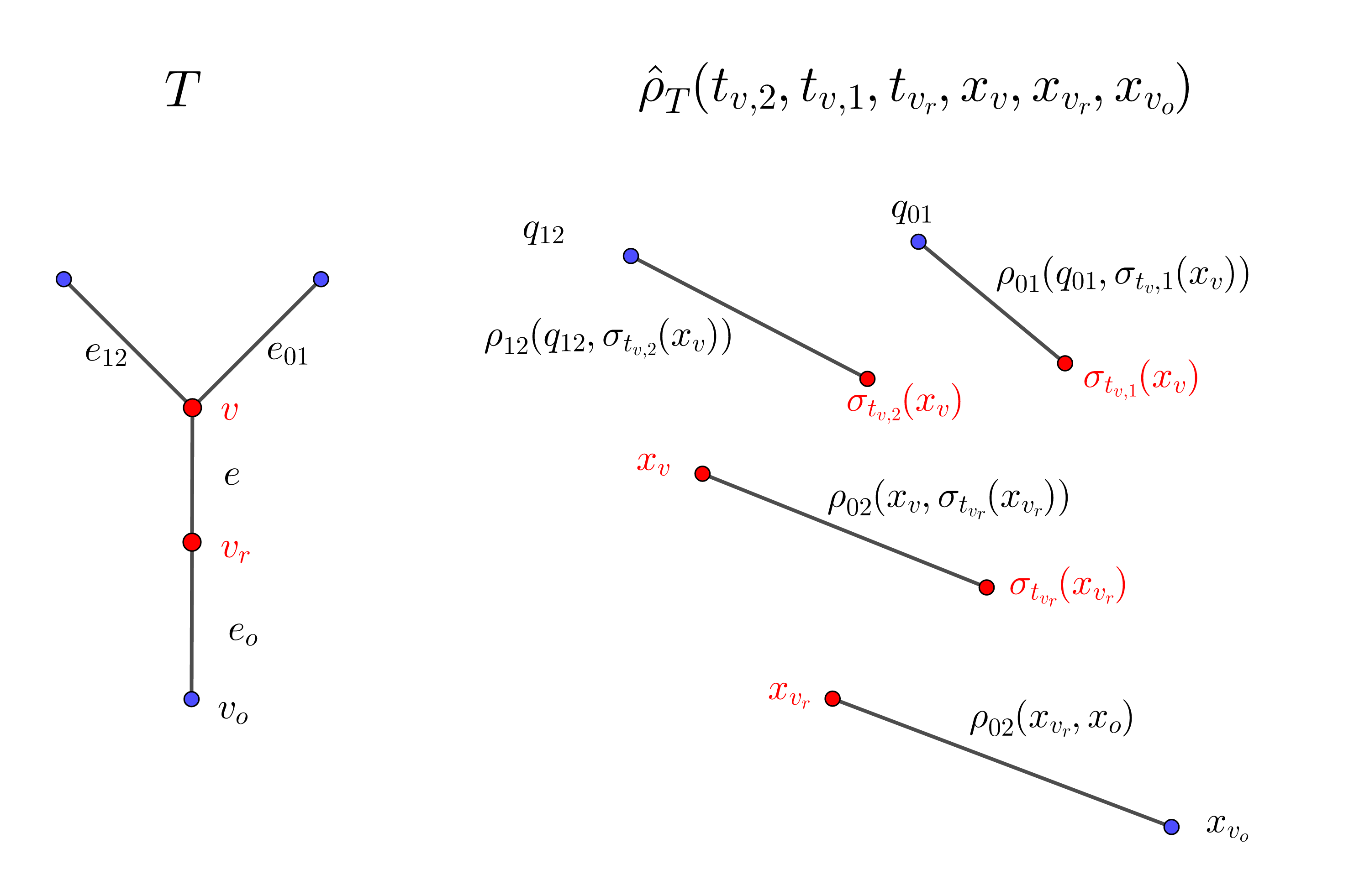 Figure 1
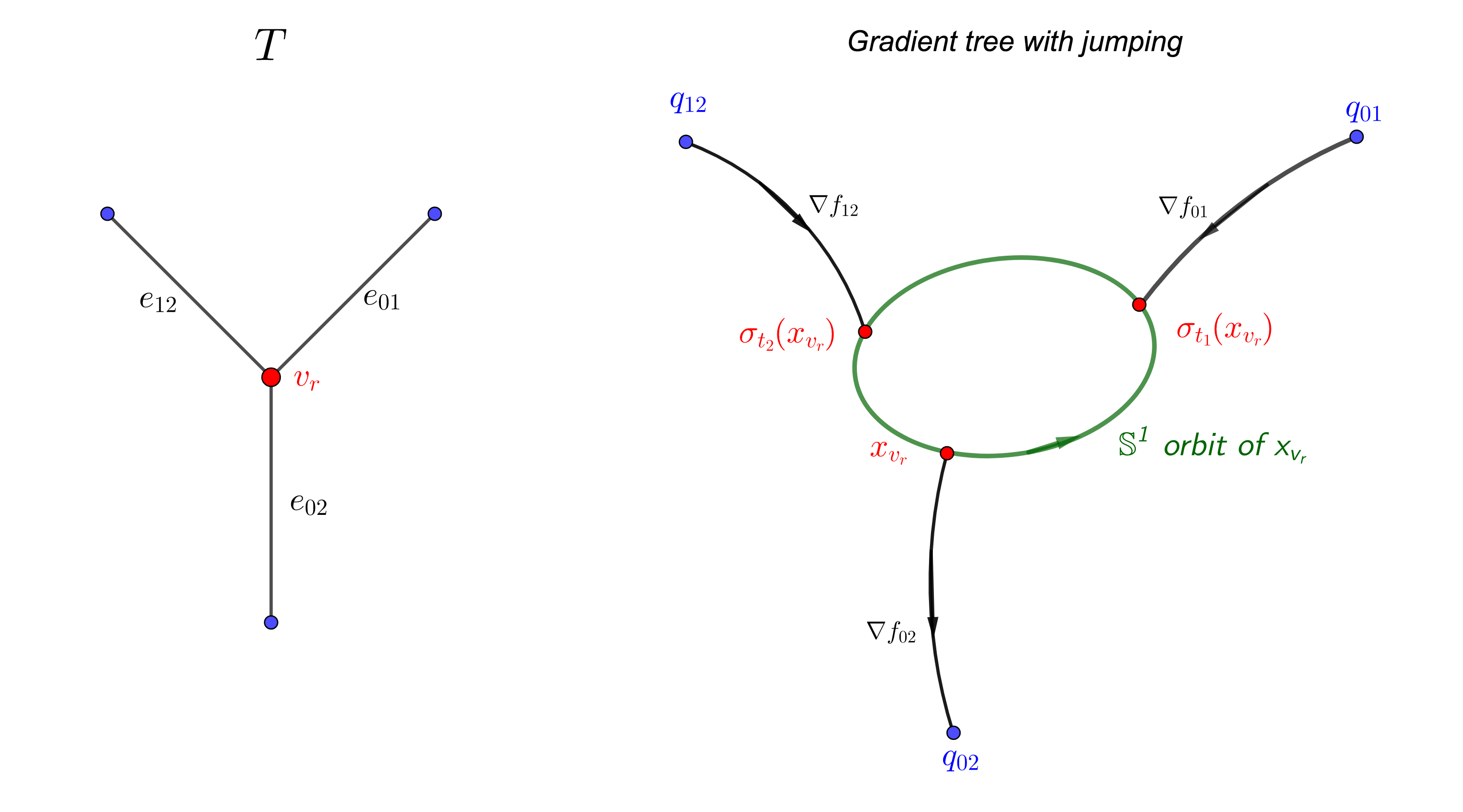 Figure 2
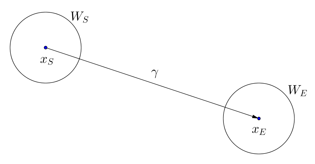 Figure 3
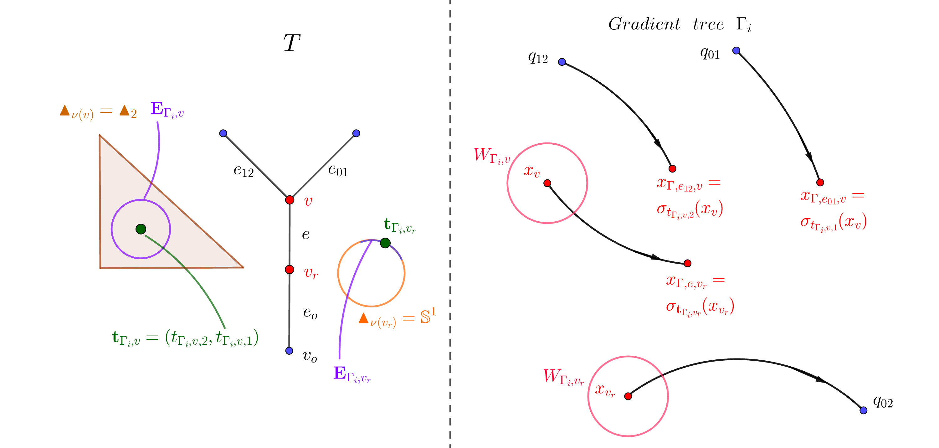 Figure 4