TL;DR
This paper introduces a computationally efficient discrete approximation to log-Gaussian Cox processes, enabling continuous spatial prediction of disease risk from aggregated count data, and demonstrates its effectiveness through simulations and real data analysis.
Contribution
The paper presents a novel discrete approximation to LGCP models that overcomes partition dependence and allows for continuous spatial prediction.
Findings
The approximation provides reliable disease risk estimates on continuous and aggregated scales.
The method outperforms traditional models in predictive accuracy.
Implementation is available in the open-source R package SDALGCP.
Abstract
In this paper, we develop a computationally efficient discrete approximation to log-Gaussian Cox process (LGCP) models for the analysis of spatially aggregated disease count data. Our approach overcomes an inherent limitation of spatial models based on Markov structures, namely that each such model is tied to a specific partition of the study area, and allows for spatially continuous prediction. We compare the predictive performance of our modelling approach with LGCP through a simulation study and an application to primary biliary cirrhosis incidence data in Newcastle-Upon-Tyne, UK. Our results suggest that when disease risk is assumed to be a spatially continuous process, the proposed approximation to LGCP provides reliable estimates of disease risk both on spatially continuous and aggregated scales. The proposed methodology is implemented in the open-source R package SDALGCP.
Click any figure to enlarge with its caption.
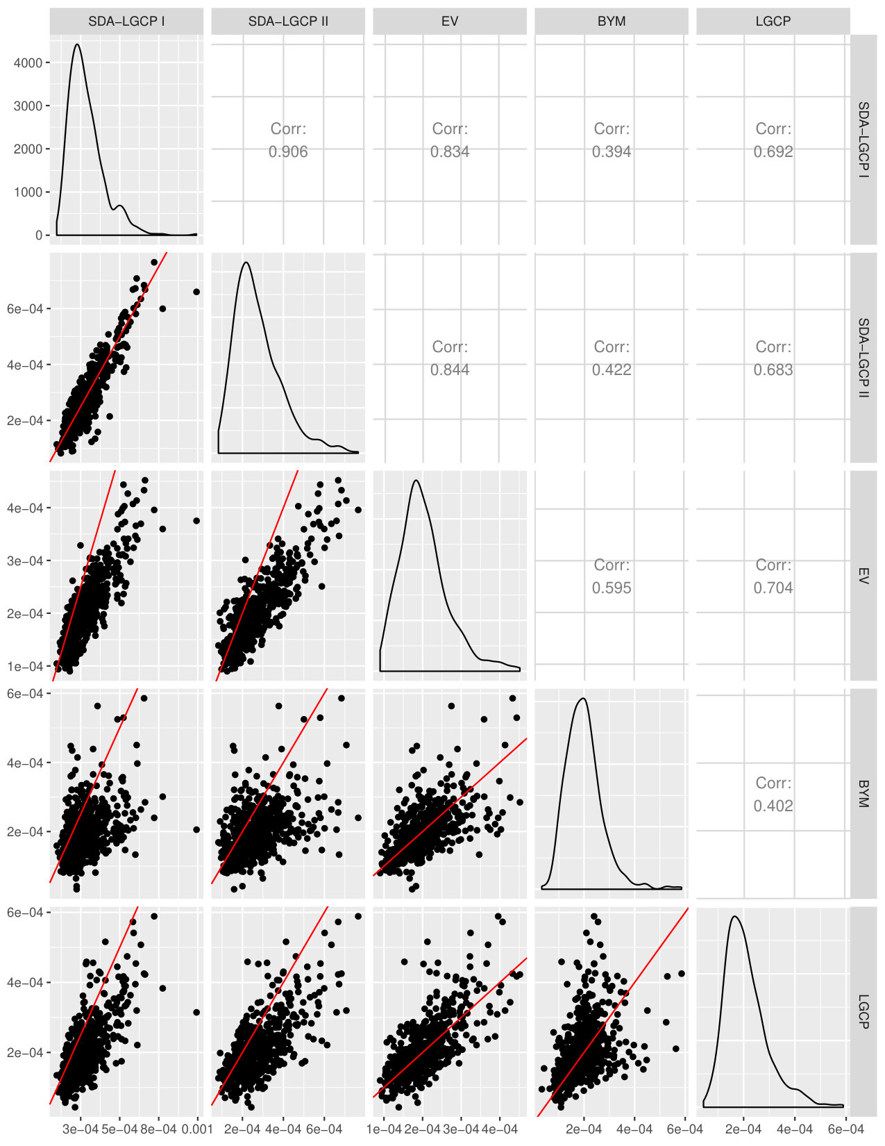 Figure 1
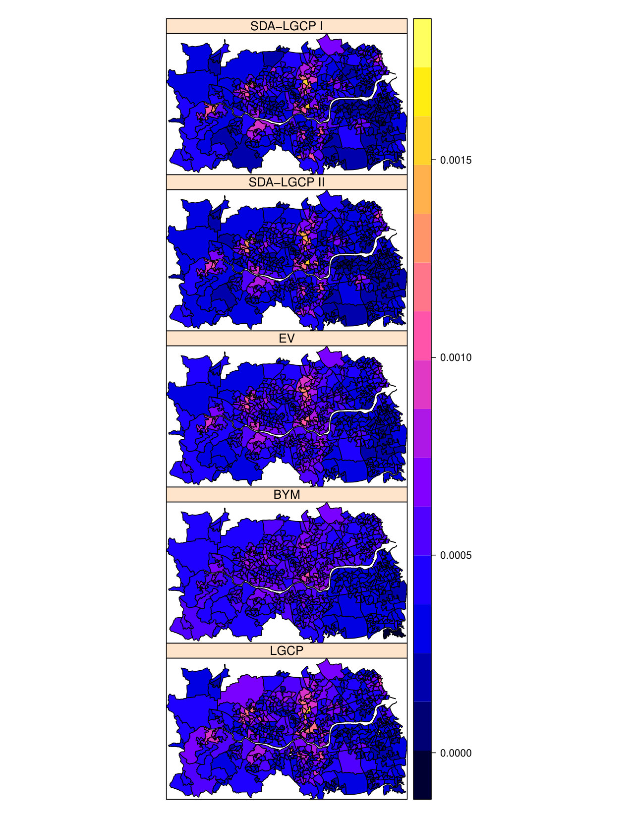 Figure 2
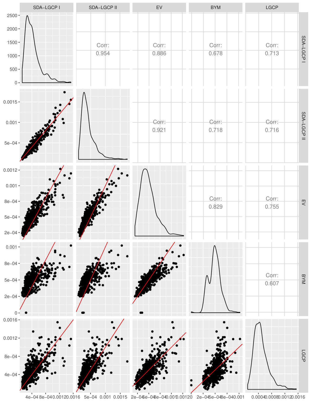 Figure 3
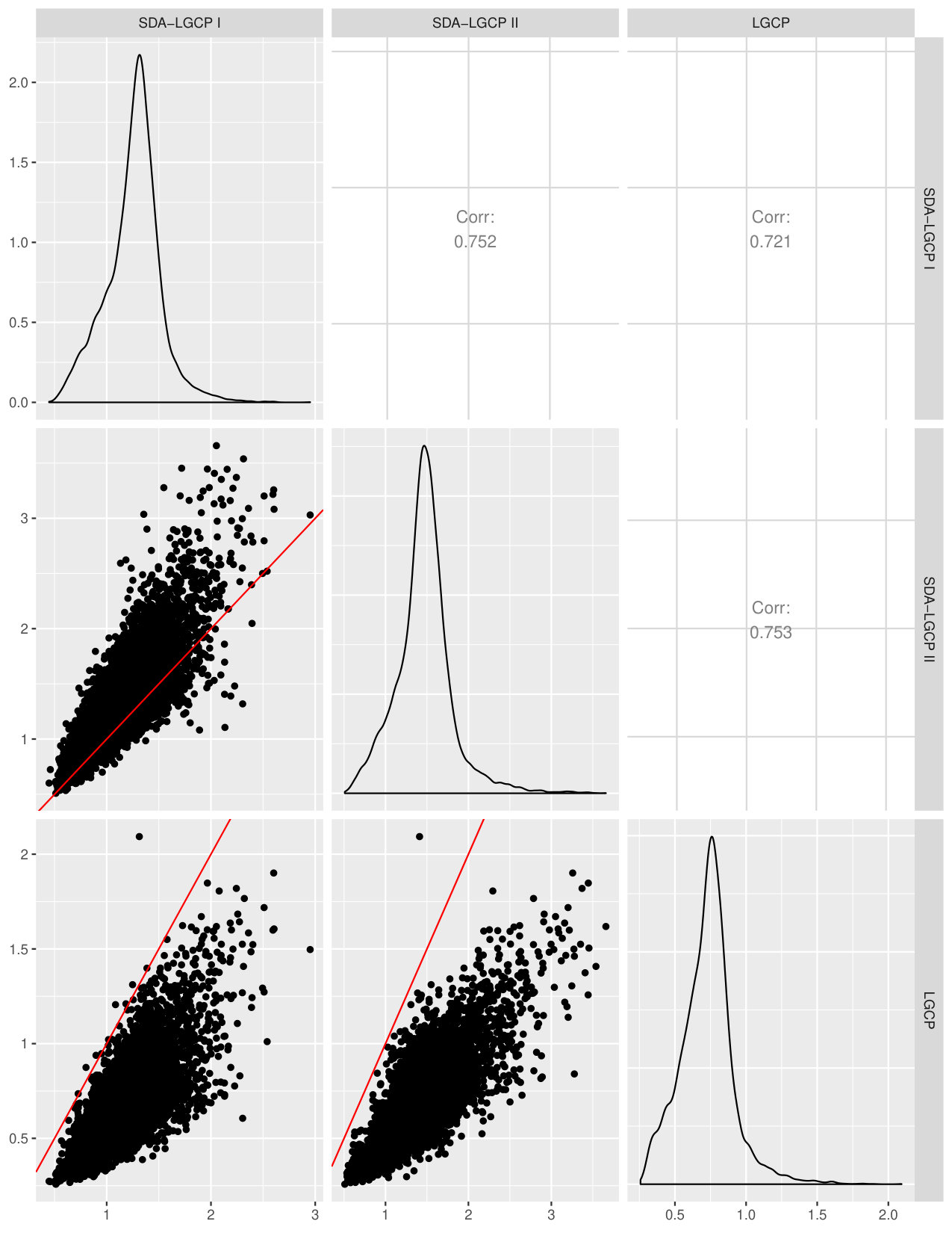 Figure 4
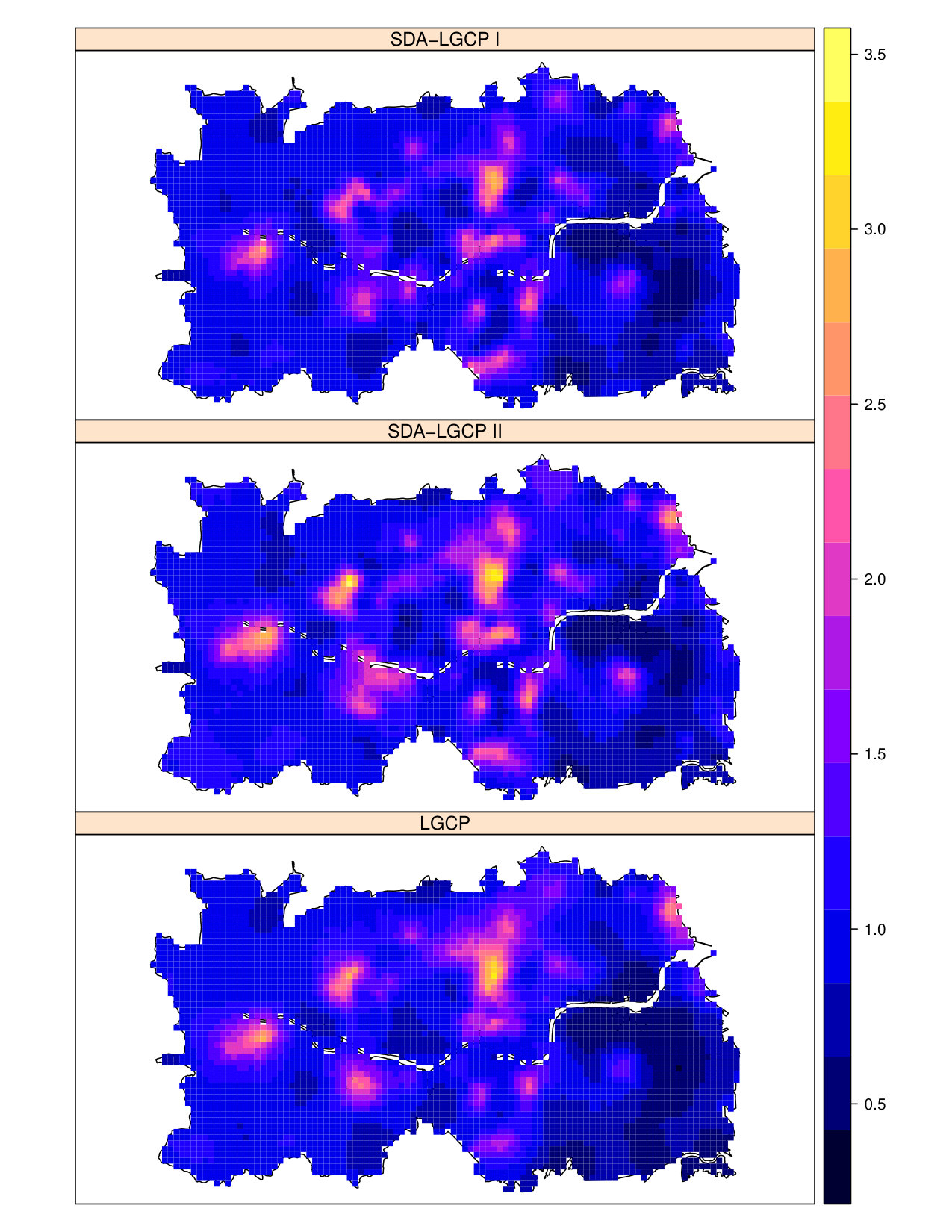 Figure 5
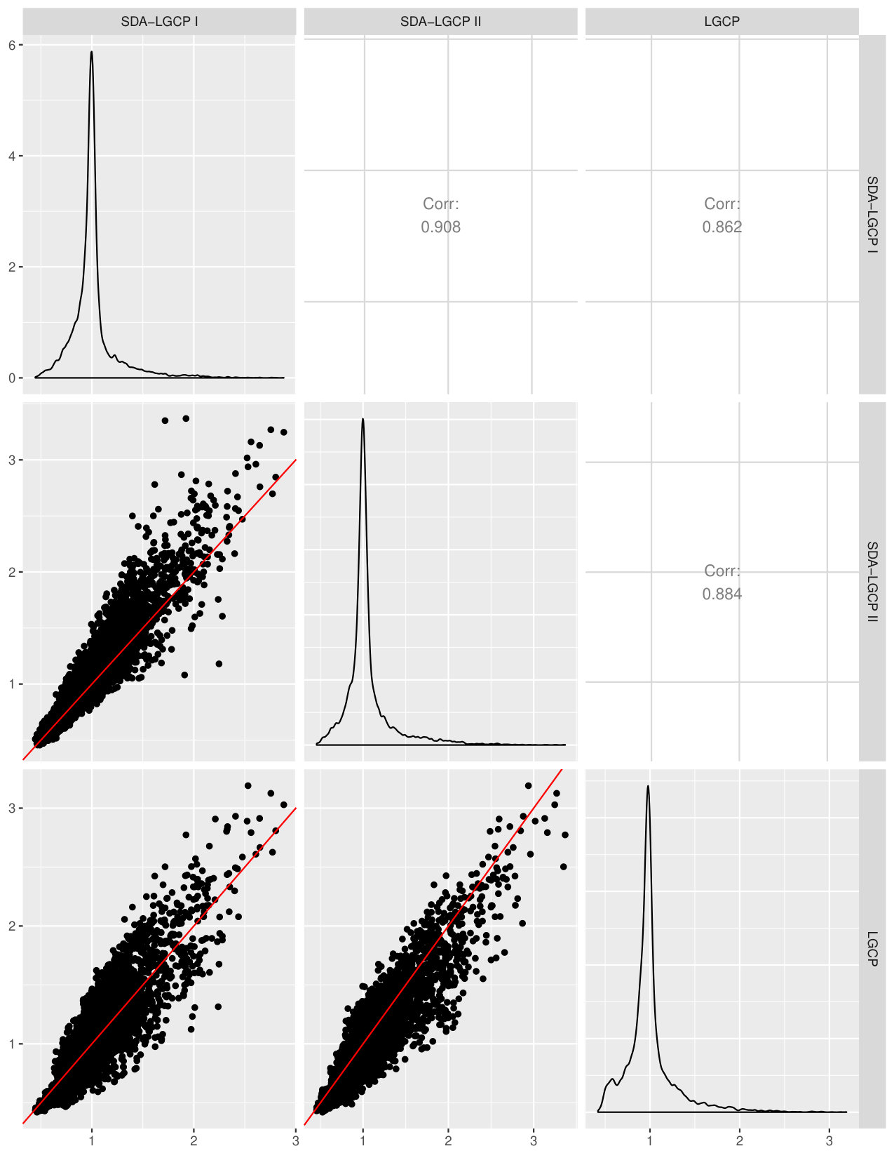 Figure 6
| SDA I | SDA II | LGCP | SDA I | SDA II | LGCP | SDA I | SDA II | LGCP | |
|---|---|---|---|---|---|---|---|---|---|
| Bias | -0.006 | -0.007 | -0.009 | -0.002 | -0.003 | -0.004 | -0.008 | -0.008 | -0.011 |
| RMSE | 0.020 | 0.021 | 0.022 | 0.003 | 0.004 | 0.006 | 0.027 | 0.029 | 0.030 |
| WPI | 0.015 | 0.016 | 0.017 | 0.002 | 0.003 | 0.004 | 0.026 | 0.028 | 0.028 |
| 95%CP | 0.940 | 0.942 | 0.948 | 0.942 | 0.943 | 0.952 | 0.943 | 0.944 | 0.945 |
| SDA I | SDA II | LGCP | SDA I | SDA II | LGCP | SDA I | SDA II | LGCP | |
|---|---|---|---|---|---|---|---|---|---|
| Bias | -0.575 | -0.582 | -0.566 | 0.842 | 0.965 | -0.108 | 0.299 | 0.316 | 0.227 |
| RMSE | 2.590 | 2.800 | 0.045 | 0.439 | 0.531 | 0.005 | 2.070 | 2.260 | 0.002 |
| WPI | 2.525 | 2.739 | 0.564 | 0.719 | 0.806 | 0.108 | 2.048 | 2.238 | 0.227 |
| 95%CP | 0.988 | 0.990 | 0.940 | 0.979 | 0.983 | 0.948 | 0.975 | 0.982 | 0.942 |
| Model | Parameter | Estimate | 95 CI |
|---|---|---|---|
| SDA I | 1.043 | (0.907, 1.180) | |
| 742.857 | (453.153, 1005.405) | ||
| -8.080 | (-8.248, -7.912) | ||
| 0.008 | (0.004, 0.011) | ||
| SDA II | 1.020 | (0.898, 1.142) | |
| 857.143 | (489.590 1037.638) | ||
| -7.876 | (-8.029, -7.722) | ||
| 0.006 | (0.002, 0.010) | ||
| EV | 0.316 | (0.246, 0.369) | |
| 525.570 | (367.719, 949.950) | ||
| -8.069 | (-8.177, -7.957) | ||
| 0.009 | (0.006, 0.011) | ||
| BYM | 0.108 | (0.012, 0.470) | |
| 0.023 | (0.003, 0.173) | ||
| -7.917 | (-8.167, -7.694) | ||
| 0.007 | (0.001, 0.014) | ||
| LGCP | 0.479 | (0.237, 0.914) | |
| 1163.877 | (528.618, 1967.756) | ||
| -19.333 | (-19.738, -19.013) | ||
| 0.008 | (0.001, 0.015) |
Peer Reviews
No public reviews on file for this paper yet. If you reviewed it on a platform where reviews are public (OpenReview, ICLR, NeurIPS, ICML), you can paste yours below so the community can read it here.
Code & Models
Videos
No videos yet. Explain this paper in a talk, walkthrough, or lecture? Add one.
A Spatially Discrete Approximation to Log-Gaussian Cox Processes for Modelling Aggregated Disease Count Data
Olatunji Olugoke Johnson, Peter Diggle and
Emanuele Giorgi
CHICAS, Lancaster Medical School,
Lancaster University, Lancaster, UK
Abstract
In this paper, we develop a computationally efficient discrete approximation to log-Gaussian Cox process (LGCP) models for the analysis of spatially aggregated disease count data. Our approach overcomes an inherent limitation of spatial models based on Markov structures, namely that each such model is tied to a specific partition of the study area, and allows for spatially continuous prediction. We compare the predictive performance of our modelling approach with LGCP through a simulation study and an application to primary biliary cirrhosis incidence data in Newcastle-Upon-Tyne, UK. Our results suggest that when disease risk is assumed to be a spatially continuous process, the proposed approximation to LGCP provides reliable estimates of disease risk both on spatially continuous and aggregated scales. The proposed methodology is implemented in the open-source R package SDALGCP.
Keywords: disease mapping; geostatistics; log-Gaussian Cox process; Monte Carlo maximum likelihood.
1 Introduction
In this paper our concern is to make inference on a spatially continuous disease risk surface using aggregated counts of reported disease cases, say , over regions forming a partition of a geographical area of interest . In this context, information on risk factors and on the population at risk may also be available, possibly at different spatial scales. We shall denote these by and , respectively, when available on a spatially continuous scale, and by and when they are spatially aggregated.
Existing methods from small area estimation (SAE) only allow spatial prediction at the aggregated level of the regions and are usually based on a Gaussian Markov random field (GMRF) structure. (Besag,, 1974; Rue and Held,, 2005) Typically, non-zero elements of the precision matrix of a GMRF are restricted to contiguous pairs of the . Hence, the formulation and interpretation of a GMRF is tied to the specific partition of , which will usually have been drawn up for administrative, historical, or other reasons unrelated to the disease aetiology. The use of such models also becomes impractical when the spatial units change over time. Wall Wall, (2004) points out that the use of GMRFs is especially problematic when dealing with irregular geometries, which can induce counter-intuitive forms for the correlation structure between variables associated with the .
The geostatistical paradigm, unlike SAE, treats disease risk as a spatially continuous phenomenon irrespective of the data-format. Diggle et alDiggle et al., (2013) argue that the analysis of spatially aggregated counts can be regarded as a special case of the class of geostatistical problems and propose to model the as an aggregated realisation of a Log-Gaussian Cox process (LGCP). Unlike GMRFs, LGCPs allow for prediction of disease risk at any spatial scale, while avoiding the ecological fallacy.(Wakefield and Shaddick,, 2006) However, fitting of LGCP models using the aggregated counts is computationally demanding due to the iterative imputation of the unobserved locations for each reported case within a region .(Li et al.,, 2012)
In this paper, our objective is to develop a computationally efficient approximation to LGCPs in order to predict disease risk at any desired spatial scale. We argue that this provides a more realistic alternative to GMRF models when LGCPs are not computationally feasible, and can also be used as an exploratory tool in order to inform more complex modelling approaches based on LGCPs.
In Section 2 of the paper, we review existing methods for modelling spatially aggregated disease counts. In Section 3, we develop a computationally efficient spatially discrete approximation to LGCP models. In Section 4 we carry out a simulation study to investigate the predictive performance of the proposed approximation and compare this with an exact fitting algorithm for LGCP models. In Section 5 we show an application of the method to a data-set on primary biliary cirrhosis (PBC) incidence in Newcastle, UK. Section 6 is a concluding discussion on the advantages and limitations of the proposed approach.
The method has been implemented in the open-source R package SDALGCP,(Johnson et al.,, 2018) available from the Comprehensive R Network Archive. The R code for reproducing the results of Section 5 is available as supplementary material.
2 Existing methods for modelling spatially aggregated disease counts data
2.1 Gaussian Markov random field models
Let denote the reported disease count in region . Conditionally on a zero-mean Gaussian process , assume that the are mutually independent Poisson random variables with expectations
[TABLE]
where is a vector of regression coefficients and is the population count or a standardised expectation of the number of cases, taking into account the demographics of the population in subregion but assuming that risk is otherwise spatially homogeneous. Spatially discrete models are then developed by specifying the precision matrix for the Gaussian process . Here, we focus on the two most commonly used formulations for , namely the conditional autoregressive (CAR) (leroux2000estimation) and intrinsic conditional autoregressive (ICAR) (Besag et al.,, 1991) models.
Let be a shorthand notation for “ and are neighbours”. A CAR model then assumes that
[TABLE]
where , is the spatial dependence parameter and are known quantities such that if and only if and . It follows from Brook’s Lemma (Brood,, 1964) and the Hammersley-Clifford Theorem (Besag,, 1974) that the joint distribution of is a multivariate zero-mean Gaussian distribution with covariance matrix
[TABLE]
where , while the specification of is generally tied to the specific arrangement of the partition of the region of interest. The most common approach is to set if and 0 otherwise. The matrix in (3) is then a valid covariance matrix if (Cressie,, 1993, pg. 472), where and are the minimum and maximum eigenvalues of , respectively. Scaling of the matrix so as to obtain a weighted average of the in (2) also implies that .
The ICAR model is a special case of the CAR model when in (2). Although this leads to an improper distribution for because of the singularity of its covariance matrix, the associated conditional distribution of given is proper.
2.2 Log-Gaussian Cox process models
A spatial point process is a stochastic mechanism that generates a countable set of events . The class of inhomogeneous Poisson processes with intensity is defined by the following postulates.
The number of events, , in any planar region follows a Poisson distribution with mean . 2. 2.
Conditionally on , each event in is an independent random sample from a distribution on with probability density function proportional to .
A Cox process (Cox,, 1955) is defined by a non-negative valued stochastic process such that, conditional on a realisation of , the process is an inhomogenous Poisson process with intensity . If we assume that is a Gaussian process, we obtain the log-Gaussian Cox process (LGCP); for more details on the theoretical properties of LGCPs, see Moller et alMøller et al., (1998)
Diggle Diggle et al., (2013) develop a modelling framework for aggregated disease count data using LGCPs. They assume that, conditionally on , the are mutually independent Poisson variables with means
[TABLE]
where is a vector of covariates at location with associated regression coefficients .
A first notable difference between (1) and (4) is that the latter uses spatially continuous information on the distribution of the expected cases, , hence, unlike (1), avoids the questionable assumption of a homogeneous distribution of the population at risk within . However, population density is often only available in the form of small-area population counts, implying a piece-wise constant surface . Note, however, that modelled spatially continuous maps for population density have been made freely available; see, for example, sedac.ciesin.columbia.edu/data/collection/gpw-v4.
Furthermore, unlike the spatially discrete models described in the previous section, LGCP is not tied to any particular partition of the area of interest and therefore provides a route to a solution to the problem of combining information at multiple spatial scales. However, this is offset by a substantial increase in the computational burden arising from the need to impute the unobserved locations for each of the reported cases within each of the , .(Li et al.,, 2012) In the next section, we circumvent this issue by proposing a spatially discrete approximation to which allows to model the counts as the realisation of a Poisson log-linear mixed model.
3 A spatially discrete approximation to Log-Gaussian Cox processes
Let be a positive function with domain , such that . Using the same notation as in Section 2.2, we approximate the conditional log-intensity of an LGCP as piecewise constant by taking its weighted average over to give
[TABLE]
where is a vector of regression coefficients for the aggregate explanatory variables and is a Gaussian process. The rationale for using the weighting function is to account for the potential non-homogeneous distribution of disease cases within a region . For example, a larger number of cases may concentrate in more densely populated areas, thus a natural choice for would be to set this equal to with , if is available. If is instead unavailable, a pragmatic approach would be to set .
Following from (5), we obtain the following approximation for the conditional mean of the counts
[TABLE]
The joint distribution of is multivariate Gaussian with zero mean and covariance function
[TABLE]
where is the Euclidean distance and is the isotropic and stationary covariance function of indexed by the parameter . Hence, the resulting model (6) falls under the class of generalized linear mixed models. Also, note that the variance of depends on the size and shape of , with larger regions leading to smaller variances.
We now provide further details on the computation of the covariance function in (7). Among the class of isotropic and stationary covariance functions for in (6), one of the most commonly used is the Matérn covariance function,(Stein,, 2012) which has expression
[TABLE]
where is the Euclidean distance between any two locations and , is the variance, is a scale parameter that regulates the rate at which the spatial correlation decays for increasing distance , is the shape parameter that determines the differentiability of the process and is the modified Bessel function of the second kind of order . Estimating reliably requires a large amount of densely sampled data, which in this context is not available. As shown by Zhang,zhang2004inconsistent not all of the three parameters , and can be consistently estimated under in-fill asymptotics, and in practice this translates to often being poorly identified. This issue is likely to be further exacerbated in this context. As a pragmatic approach, we then set which reduces (8) to
[TABLE]
corresponding to a mean-square continuous process.
We approximate (7) as a discrete sum over and randomly chosen points in and to give
[TABLE]
To attain a good spatial coverage of and , we propose to draw each of the and in the above equation using a class of inhibition processes (Diggle,, 2013, pp. 110-116) which combine simple sequential inhibition with rejection sampling. More specifically, we proceed through the following steps.
Compute . 2. 2.
Generate over from a homogeneous Poisson process with intensity . 3. 3.
Compute . 4. 4.
Generate a sample from the uniform distribution on . 5. 5.
If , set if ; for and given , set if and falls at the intersection of and . Otherwise, reject . 6. 6.
Repeat 2 to 5, until .
To identify a suitable value for (the total number of generated points within ), a possible solution is to use the packing density for a sequential inhibitory point process given by
[TABLE]
where is the minimum permissible distance between points. The maximum possible value for is obtained by close-packed discs whose centres form an equilateral triangular lattice with sides of length . Through a simulation study, Tanemura Tanemura, (1979) suggested to set in order to achieve good spatial coverage in a relatively small number of iterations. Once and are fixed, we can then obtain through equation (10).
An alternative solution is to leave choose as a function of using the following adaptive algorithm.
For a given , initialize a batch size and a relative tolerance ; 2. 2.
Locate quadrature points with packing intensity , evaluate the integral in (3) and denote its value as ; 3. 3.
Add points using a packing intensity , re-evaluate the integral and denote its value as ; 4. 4.
If , stop the algorithm. Otherwise, set , add points with and repeat until
Since is almost always unknown, the adaptive algorithm becomes more computationally demanding, especially in the case of a large number of regions in the study domain and for small values of which require a finer grid for a satisfactory approximation of (7). When fitting the model in (6) (see next section for more details), our recommendation is to use the non-adaptive algorithm first, in order to locate the likely value of , and then to run a final estimation using the adaptive algorithm. In the application in Section 5, the adaptive algorithm increases the elapsed time by about 10 minutes (592 seconds) on a laptop with 7.6GiB memory and processor. Furthermore, in order to reduce the computational burden, we propose to discretise over a finite set of values and pre-compute the covariance matrix as defined by (3) for each of the pre-defined values. To obtain a 95 confidence interval for , we then compute the profile likelihood over the discrete set and interpolate it using a natural cubic spline. In our experience, the fineness of the discretisation does not have tangible effects on the spatial predictions but, instead, directly affects the goodness of the numerical approximation of the confidence interval based on the profile likelihood.
3.1 Monte Carlo maximum likelihood
We carry out parameter estimation for the model in (6) using the Monte Carlo maximum likelihood (MCML) method.(Christensen,, 2012)
Let be a shorthand notation for “the density function of ”. Let and linear predictor ; it then follows that conditionally on , the joint distribution of is
[TABLE]
where
[TABLE]
Let denote the vector of the model parameters, then the likelihood function for is obtained by integrating out , i.e.
[TABLE]
In (11) is a multivariate Gaussian distribution function with mean , where denotes a matrix of explanatory variables, and covariance matrix , whose -th entry is given by (7). To reduce the computational burden accrued from the numerical approximation (3), we restrict the maximization of (11) to a finite set of predefined values for and, for each of these, pre-compute the covariance matrix together with its inverse, determinant and Cholesky decomposition.
Since the high-dimensional integral in (11) cannot be solved analytically, we use Monte Carlo methods for the approximation of the likelihood. Let denote our best guess of . We re-write (11) as
[TABLE]
where the expectation is taken with respect to the conditional distribution of given with parameters vector . We provide the proof of this in Appendix A of the supplementary material.
To generate samples, say , from the conditional distribution of given , we use a Monte Carlo Markov chain (MCMC) algorithm implemented in the Laplace.sampling.MCML function in the PrevMap package.(Giorgi and Diggle,, 2017) This function uses a Metropolis-adjusted Langevin MCMC algorithm to update the standardised vector of random effects, , where and are the mode and the inverse of the negative Hessian of at . We can then approximate the likelihood function in (12) as
[TABLE]
As , in the above equation, converges to . Geyer and Thompson, (1992); Geyer, (1994, 1996)
Finally, we maximize (13) using a constrained quasi-Newton optimization algorithm, implemented in the nlminb function in the R software environment, by providing analytical expressions for the first and second derivatives of (13) with respect to . If denote the resulting MCML estimate, we then set and repeat the previous steps until convergence.
3.2 Continuous spatial prediction
We now consider the problem of carrying out spatial prediction of at a pre-defined location within the study area . Using the same notation as in the previous section, we first note that
[TABLE]
Hence, we sample from using the following two-step procedure: (1) draw samples , for from using the MCMC algorithm described in the previous section; (2) for each , for simulate from , a Gaussian distribution with mean and variance where , and we use (3) to approximate the integral. The resulting samples from can then be used to compute non-linear properties of and to summarise these using, for example, predictive means and standard errors.
4 Simulation Study
We now conduct a simulation study to assess the predictive performance of the proposed approximation in (3) when the underlying process is an LGCP model.
We simulate data-set of counts using the administrative boundaries of the lower layer super output areas (LSOAs) in Newcastle-Upon-Tyne, UK, as in the application of Section 5. We specify the offsets using population density estimates from the OpenPopGrid database (Murdock et al.,, 2015) and simulate the locations of the events using an inhomogeneous Poisson process with intensity . We define three scenarios by setting the standard deviation of the Gaussian random field to and let (whose unit of measure is metres) vary over the set , which correspond to a case of small, medium and large spatial correlation, respectively. The value of the standard deviation corresponds to the posterior mean obtained from the fitted LGCP in the application to primary biliary cirrhosis data described in the next section. Finally, for each of the simulated data-sets of aggregated counts at LSOA level, we fit the following models.
- •
LGCP. We use a Bayesian data augmentation technique implemented in the lgcp package.(Taylor et al.,, 2015) We overlay a computational grid at a spacing of of metres onto the area of interest and fit the model in (4). We run 3,100,000 iterations of the MCMC algorithm with a burn-in of 100,000 samples and then retain every 300-th sample.
- •
Spatially discrete approximation (SDA) to LGCP. We fit the approximation in (3) using a population weighted average (SDA I, with ) and simple average (SDA II, with ) of the log-intensity. For both, we use the MCML method described in Section 3.1 and run 110,000 iterations of the MCMC algorithm with a burn-in of 10,000 samples and then retain every 10-th sample.
We summarise the results from the simulation study through the bias, root-mean-square-error (RMSE), width of the predictive interval (WPI) and the 95 coverage probability (CP) for the incidence at LSOA level, , and for the spatially continuous relative risk, . Let denote the true simulated incidence for at the -th simulation; hence
[TABLE]
[TABLE]
[TABLE]
[TABLE]
where is the mean of the predictive distribution for , is an indicator function that takes value 1 if falls inside the 95 prediction interval and 0 otherwise, and and are the upper and lower limits of the 95 prediction interval, respectively. Similarly, we compute the three indices for the relative risk by averaging each of these over the regular grid at a spacing of metres covering the whole of Newcastle-Upon-Tyne, UK.
Table 1 reports the results for the prediction of , the incidence at LSOA level. We observe that SDA I and II have a slightly lower bias and RMSE than LGCP in all three scenarios, with SDA I having the best performance. The coverage probability is close to the nominal level and the WPI is comparable for all three models.
The results for the spatially continuous relative risk, , are shown in Table 2. LGCP has the lowest bias and RMSE followed by SDA I in all three scenarios, with larger differences for and . Both SDA I and II are more conservative than LGCP and provide prediction intervals with a larger coverage than the nominal level, as the result of a large RMSE. We also observe that the use of the population weighted average in SDA I leads to a tangible reduction in RMSE and bias with respect to SDA II.
5 Application: mapping of primary biliary cirrhosis risk
We analyse incidence data on primary biliary cirrhosis (PBC) in Newcastle-Upon-Tyne, UK, obtained from the original study carried out by Princ et al.Prince et al., (2001); the data-set is freely available from the lgcp R package. The data consist of geo-referenced cases of definite or probable PBC between 1987 and 1994. The objective of this analysis is to quantify the difference in the predictive inferences between the gold-standard LGCP model and the proposed spatially discrete approximation (or SDA), on PBC incidence at LSOA level and the spatially continuous relative risk surface. In the case of SDA, we fit the population weighted (SDA I) and simple average (SDA II) versions described in the previous section. We also consider the exponential variogram (EV) model proposed by WallWall, (2004) consisting of a geostatistical Poisson model for the counts whose spatial structure is defined using the centroids of each LSOA. Finally, we fit the Besag, York and Mollié Besag et al., (1991) (BYM) model, one of most commonly used approaches in small area estimation, with linear predictor
[TABLE]
where is a zero-mean intrinsically autoregressive process with variance and is Gaussian noise with variance .
In all five models, we use the index of multiple deprivation (IMD) as a covariate of the linear predictor. The IMD is publicly available from the UK Government online archives (webarchive.nationalarchives.gov.uk). The regression coefficients for the IMD are denoted by in the LGCP model and by in the BYM, EV and SDA models, with corresponding to the intercept and the effect of IMD.
For the SDA models, we run 110,000 iterations of the MCMC algorithm with a burn-in of 10,000 samples, and then retain every 10-th sample. We discretise using 100 equally spaced values between 50 and 2000 meters.
For the LGCP model, we specify independent priors as follows: , and . We run 3,100,000 iterations of the MCMC algorithm with a burn-in of 100,000 samples and retain every 3000-th sample so as to obtain a set of 1,000 weakly dependent samples.
Fitting of the BYM model using CARBayescarbayes is carried out by iterating the MCMC algorithm 1,100,000 times with a burn-in of 100,000 samples and retaining every 100-th sample.
Finally, for the EV model which fit using the spBayes spbayes R package, we specify an inverse-Gamma prior on the variance parameter with shape parameter 1 and scale parameter 2. The spatial scale parameter is assigned a uniform prior in the interval . For the regression coefficients , we use a flat prior. We run 1,100,000 iterations of the MCMC algorithm with a burn-in of 100,000 samples and retain every 40-th sample.
Trace-plots and correlograms are used to assess convergence of the MCMC algorithms in each of the fitted models. These are reported in the Appendix, from section B to E, and all indicate a good mixing of the resulting MCMC samples.
Tables 3 reports the point and interval estimates for the parameters of each of the fitted models. We observe that the differences amongst the point estimates of the regression coefficients from the five models are small.
Figure 1 shows a map of the estimated PBC incidence at LSOA level from the five models. The spatial spatial pattern estimated by each of these is comparable, as indicated by the scatter plots of Figure 2. The same consideration holds for the predictive standard errors (Figure 3). More specifically, the estimated incidence from the LGCP model has a correlation of about 0.7 with the other models, expect the BYM model for which the correlation is about 0.6. The good performance of the EV model can be explained by the fact that, in this scenario, the size of most of the LSOAs is small relative to the range of the spatial correlation, hence the use of the centroid becomes less problematic.
Figure 4 shows the map of the estimated continuous relative risk surface over a meters regular grid covering the whole of the study area. The scatter plots (Figures 5 and 6) indicate that the point estimates from the LGCP and the SDA approach are strongly similar, with a correlation of 0.862 between SDA I and LGCP and of 0.884 between SDA II and LGCP. However, we also observe that the standard errors from SDA, both I and II, are larger than those from LGCP. This is consistent with our results from the simulation study of the previous section.
6 Discussion
In this article we have developed a spatially discrete approximation (SDA) to log-Gaussian Cox process (LGCP) models in order to carry out spatial prediction of disease risk at any desired spatial scale using spatially aggregated disease count data.
As variation in disease risk occurs in a spatial continuum irrespective of the format in which the data are available, we consider the LGCP framework to be a natural statistical paradigm for modelling aggregated disease count data. However, when computational constraints make the fitting of an LGCP infeasible, we argue that SDA provides a computationally efficient solution while respecting the spatially continuous nature of disease risk. SDA also overcomes some of the limitations inherent to other spatially discrete models, such as CAR models. In addition to providing spatially continuous predictions, SDAs can also deal with the issue of changing administrative boundaries over time and allow incorporation of covariates available at any spatial scale.
Kelsall et al Kelsall and Wakefield, (2002) developed a similar approach to the proposed SDA for modelling count data available at areal level. Specifically, by assuming an intercept-only model, they approximate (4) using a multivariate log-Gaussian distribution with mean
[TABLE]
and covariance
[TABLE]
Kelsall et alKelsall and Wakefield, (2002) then advocate the use of the log-Gaussian approximation as a Bayesian prior for spatial smoothing but no reference is made to the LGCP framework. In this paper, instead, our objective was to develop a computationally efficient approximation to the LGCP model which, in Bayesian terms, is our chosen prior for modelling disease risk.
In fitting SDA models, most of the computational burden is due to the approximation of the integral in (7), which defines the area-level correlation between the spatial random effects. In our example, the SDA model is about 5 to 15 times faster to fit than the LGCP model, depending on the number of values used to discretise the scale of the spatial correlation . To make SDA even faster, efficient approximations to Gaussian processes should also be considered (see, for example, Lindgren et allindgren2011explicit). These could be used to sample from the predictive distribution of in (5) and avoid computation of the integral in (7).
We conclude that SDA is a reliable approximation to LGCP for carrying out predictions at areal-level, both in terms of point predictions and in the quantification of uncertainty. It also provides spatially continuous predictions in disease risk that are comparable to those from LGCP, but with larger standard errors and more conservative predictions intervals.
Finally, extension to the spatio-temporal case of the method discussed in this paper is possible and is work in progress. For example, let us consider counts for the region over the time interval . Let be a spatio-temporal Gaussian process with covariance function
[TABLE]
By modelling the as realisations of a spatio-temporal log-Gaussian Cox process with conditional intensity , we can then approximate this with a spatio-temporally discrete Gaussian process , such that
[TABLE]
where the temporal innovation is modelled as a multivariate Gaussian distribution with covariance matrix given by (7). Preliminary results suggest that the reduction in computing time with respect to a spatio-temporal LGCP model is substantially larger than that observed for the purely spatial scenario presented in this paper.
Acknowledgements
We thank Dr Benjamin Taylor for his useful comment on the draft of this manuscript. We also acknowledge the travel grant from African Institute for Mathematical Sciences to OOJ.
Funding
OOJ holds a Connected Health Cities funded PhD studentship.
The reference list from the paper itself. Each links out to its DOI / PubMed record.
- 1Besag, (1974) Besag, J. (1974). Spatial interaction and the statistical analysis of lattice systems. Journal of the Royal Statistical Society. Series B (Methodological) , pages 192–236.
- 2Besag et al., (1991) Besag, J., York, J., and Mollié, A. (1991). Bayesian image restoration, with two applications in spatial statistics. Annals of the institute of statistical mathematics , 43(1):1–20.
- 3Brood, (1964) Brood, D. (1964). On the distinction between the conditional probability and the joint probability approaches in the specification of nearest-neihbor systems. Biometrika , 51:481–483.
- 4Christensen, (2012) Christensen, O. F. (2012). Monte carlo maximum likelihood in model-based geostatistics. Journal of computational and graphical statistics .
- 5Cox, (1955) Cox, D. R. (1955). Some statistical methods connected with series of events. Journal of the Royal Statistical Society. Series B (Methodological) , pages 129–164.
- 6Cressie, (1993) Cressie, N. A. (1993). Statistics for spatial data: Wiley series in probability and mathematical statistics. Applied probability and statistics, rev. edn, New York: Wiley.
- 7Diggle, (2013) Diggle, P. J. (2013). Statistical analysis of spatial and spatio-temporal point patterns . CRC Press.
- 8Diggle et al., (2013) Diggle, P. J., Moraga, P., Rowlingson, B., and Taylor, B. M. (2013). Spatial and spatio-temporal log-gaussian cox processes: extending the geostatistical paradigm. Statistical Science , pages 542–563.
