
TL;DR
This paper introduces a novel approach to causal discovery using a mixture of directed cyclic graphs (DAGs) to model complex, evolving, and population-specific causal processes, with an algorithm leveraging longitudinal data for inference.
Contribution
It proposes modeling causation with a mixture of DAGs and introduces the Causal Inference over Mixtures algorithm for longitudinal data analysis.
Findings
Improved causal inference performance over prior methods.
Effective modeling of cyclic, evolving, and population-specific causal processes.
Algorithm successfully infers causal relations from complex data.
Abstract
Causal processes in biomedicine may contain cycles, evolve over time or differ between populations. However, many graphical models cannot accommodate these conditions. We propose to model causation using a mixture of directed cyclic graphs (DAGs), where the joint distribution in a population follows a DAG at any single point in time but potentially different DAGs across time. We also introduce an algorithm called Causal Inference over Mixtures that uses longitudinal data to infer a graph summarizing the causal relations generated from a mixture of DAGs. Experiments demonstrate improved performance compared to prior approaches.
Click any figure to enlarge with its caption.
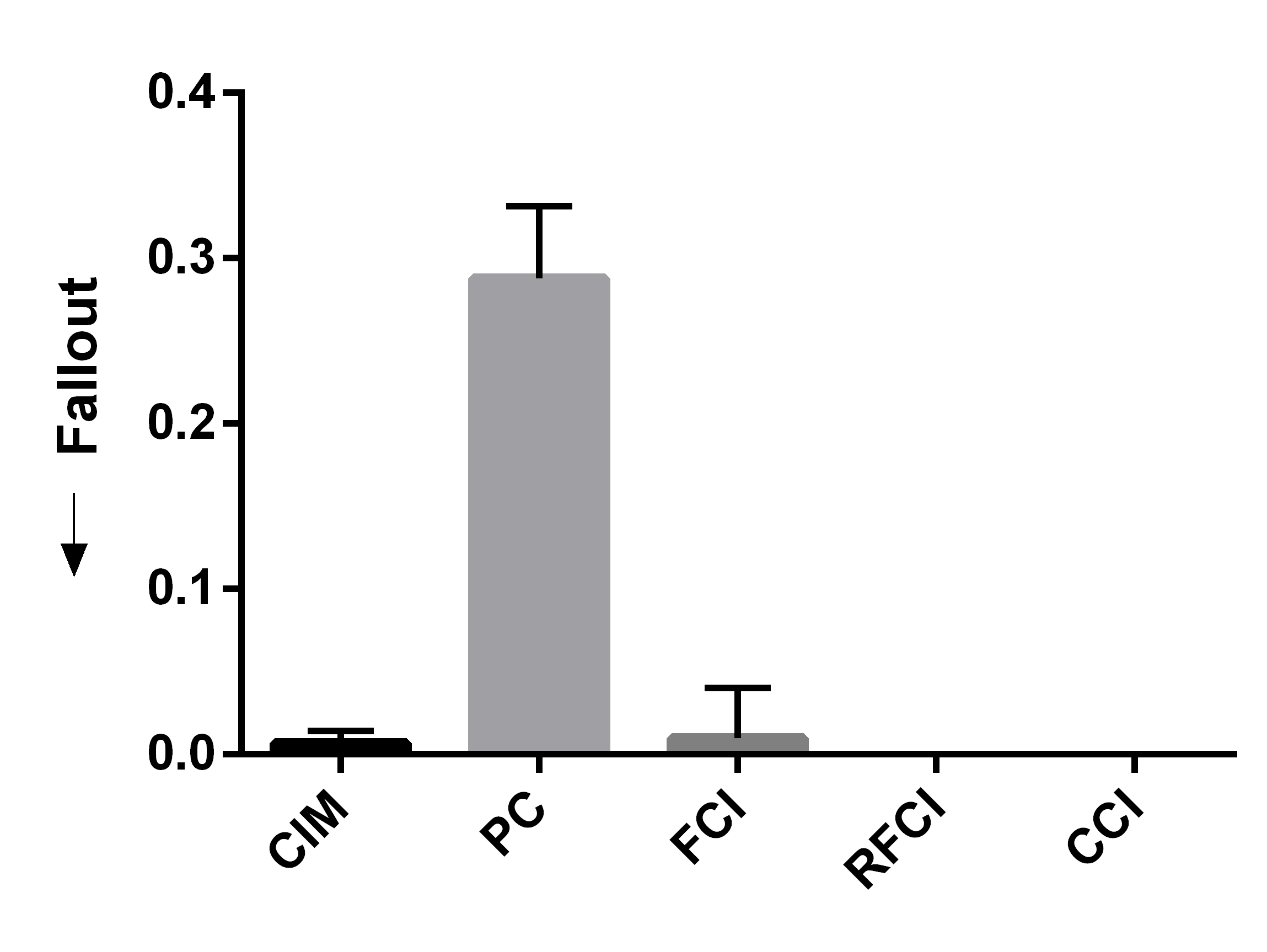 Figure 1
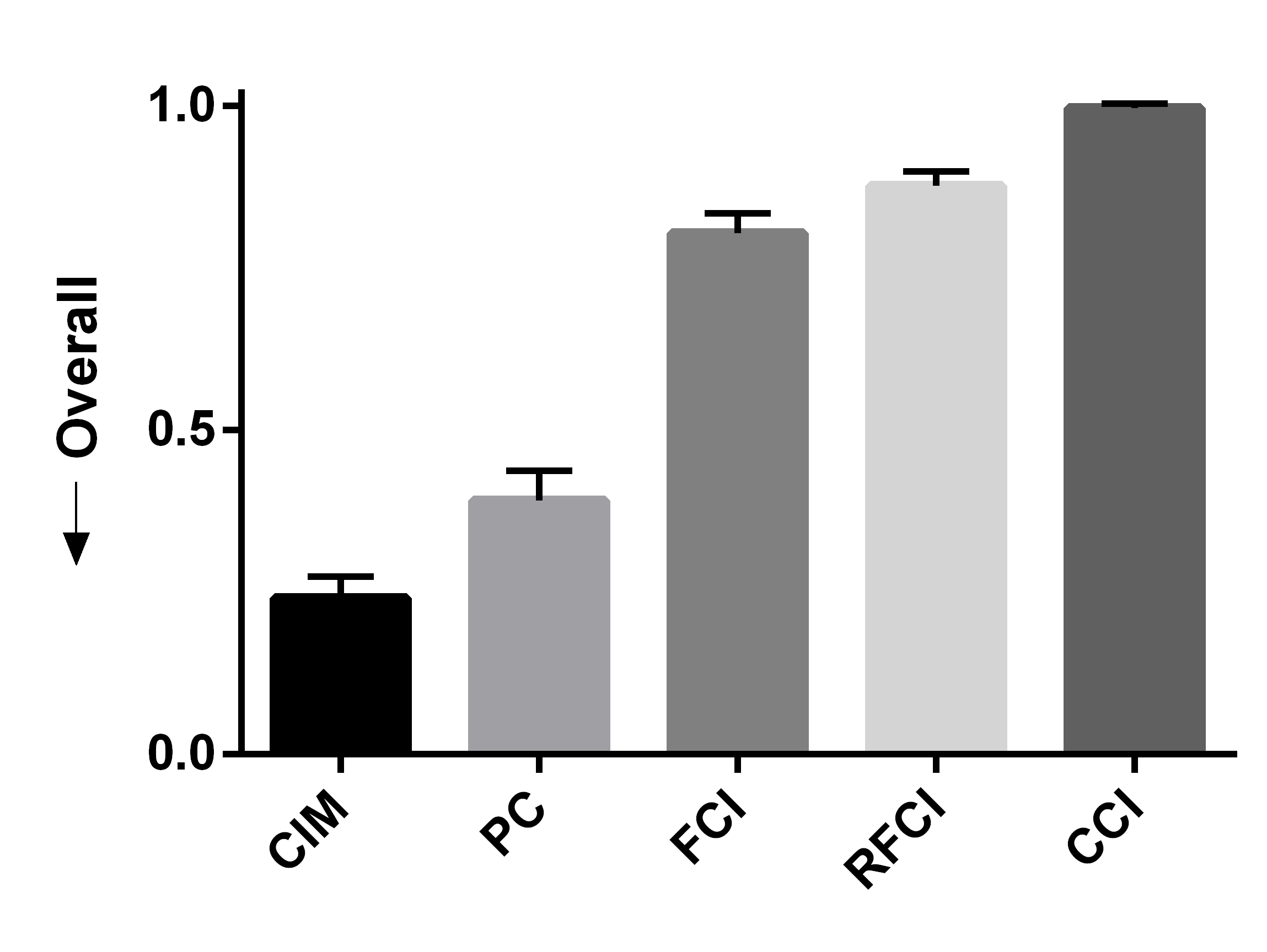 Figure 2
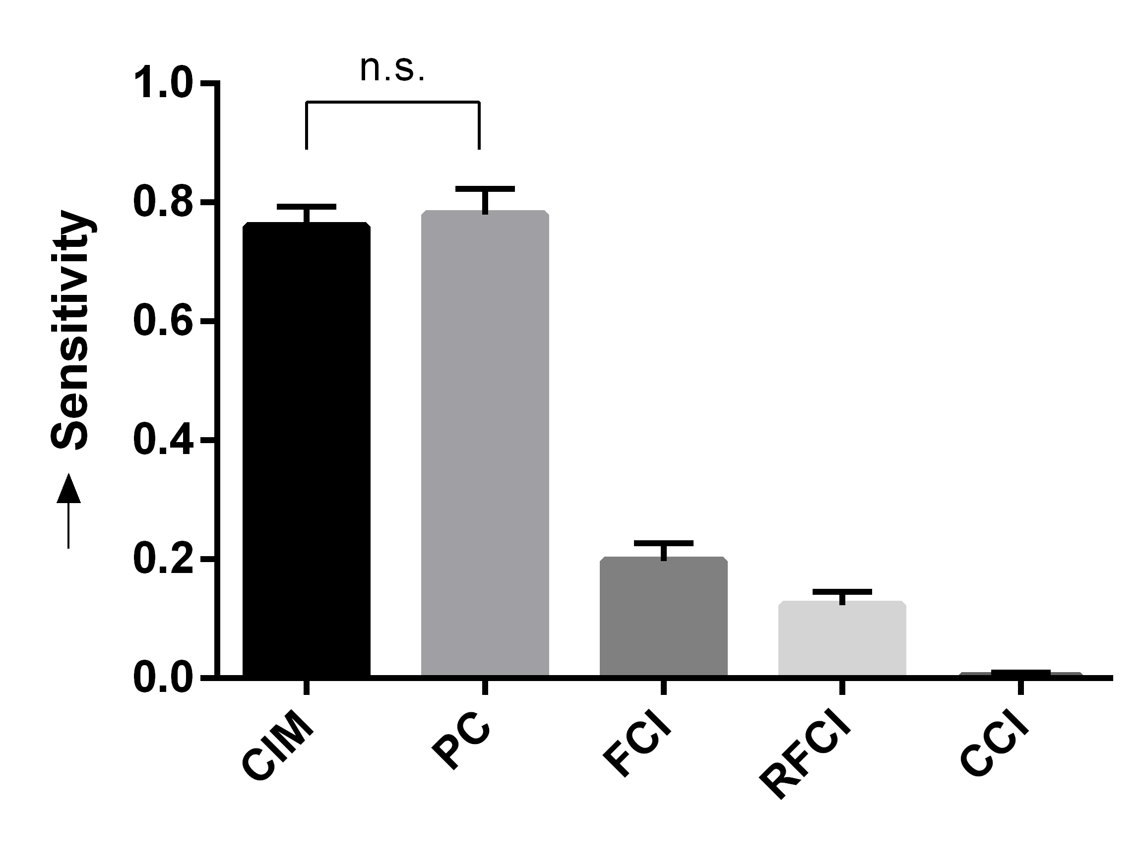 Figure 3
 Figure 4
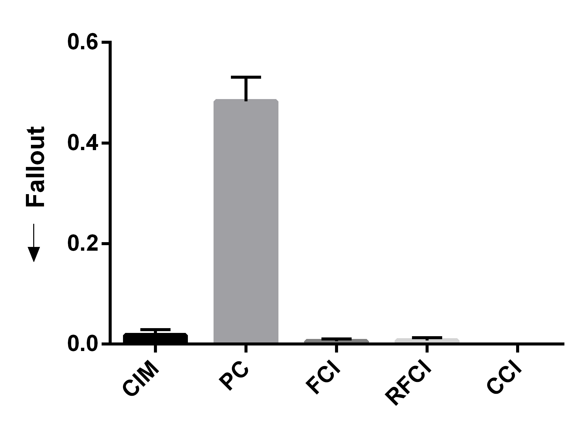 Figure 5
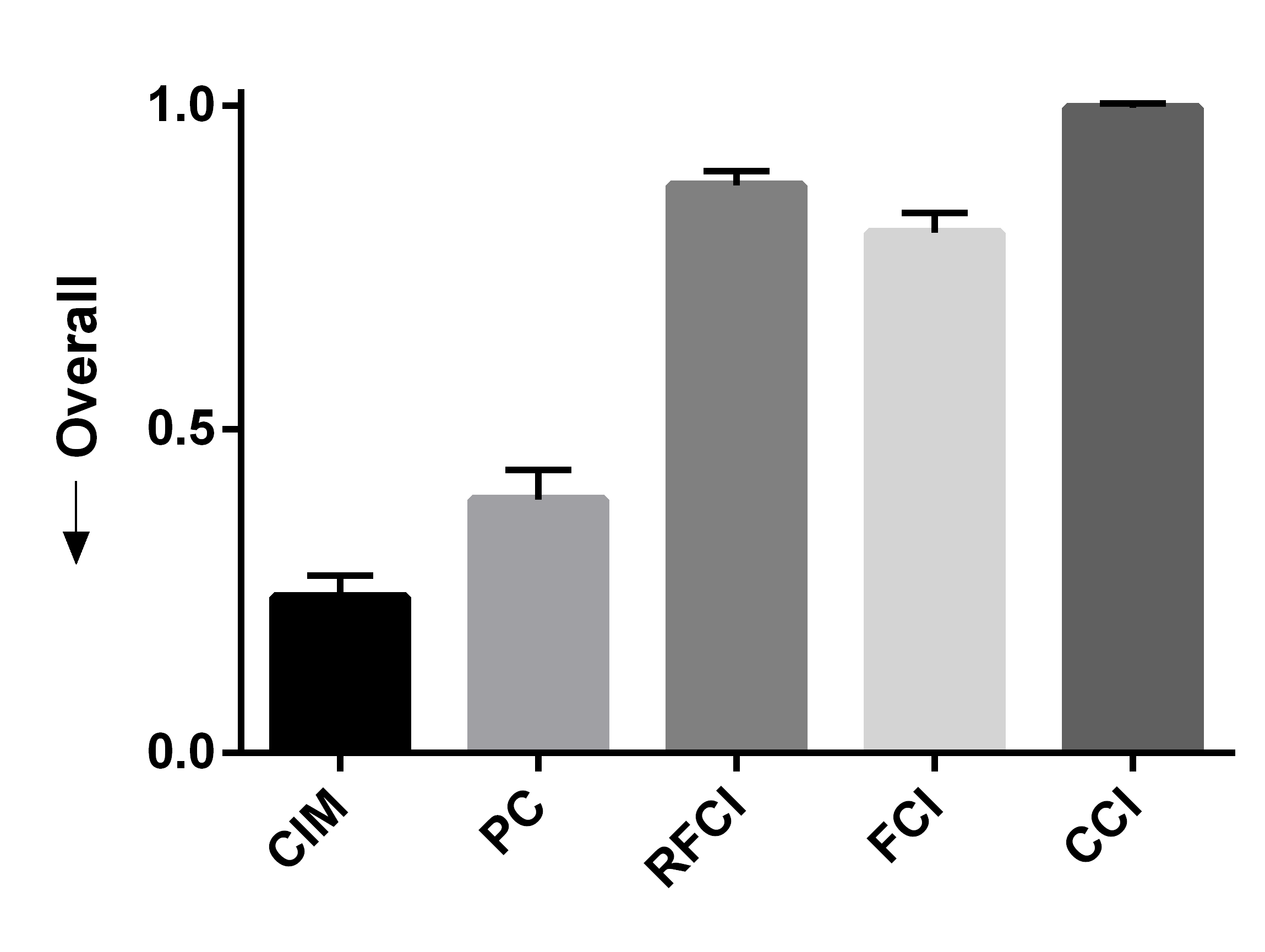 Figure 6
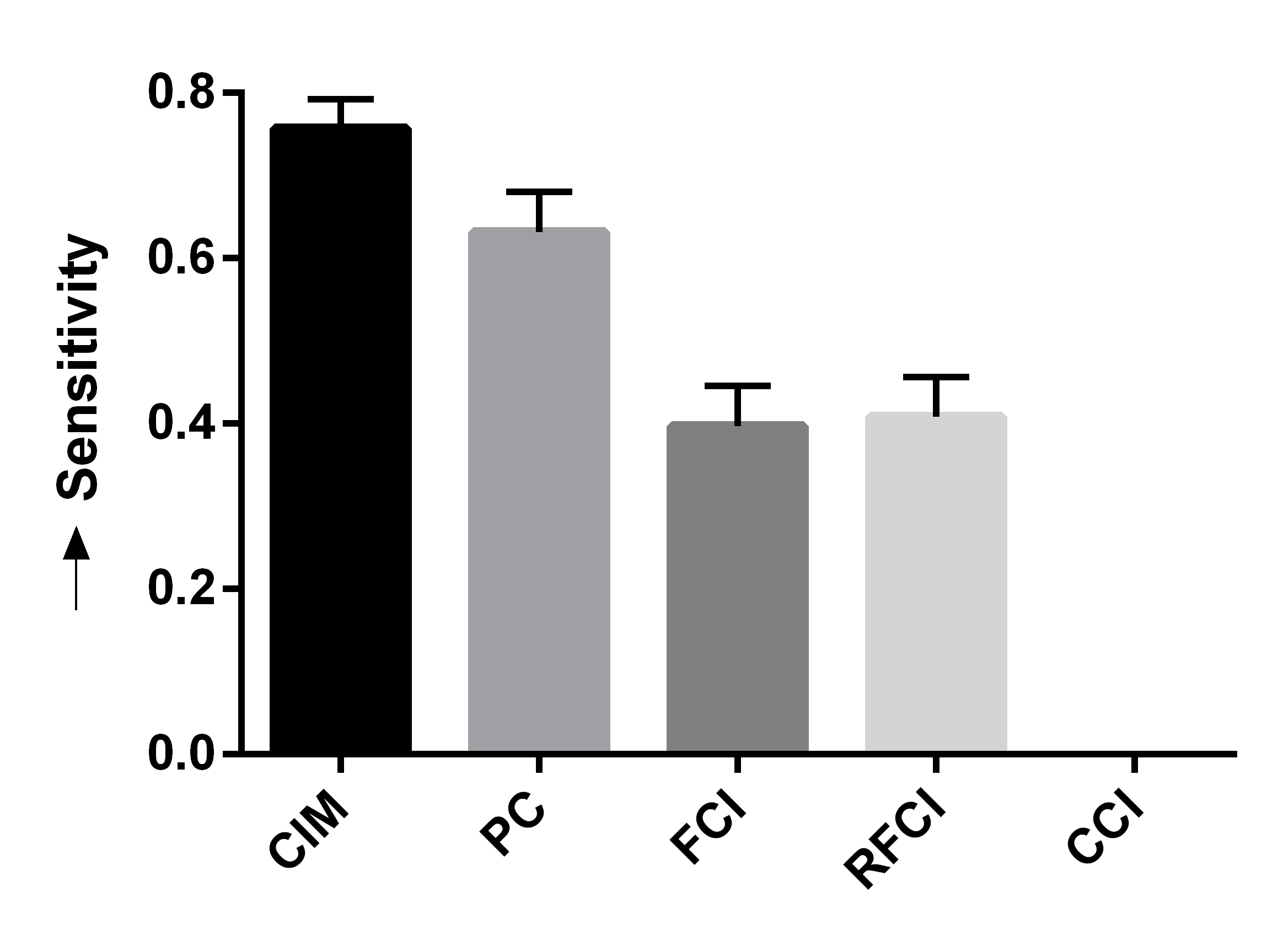 Figure 7
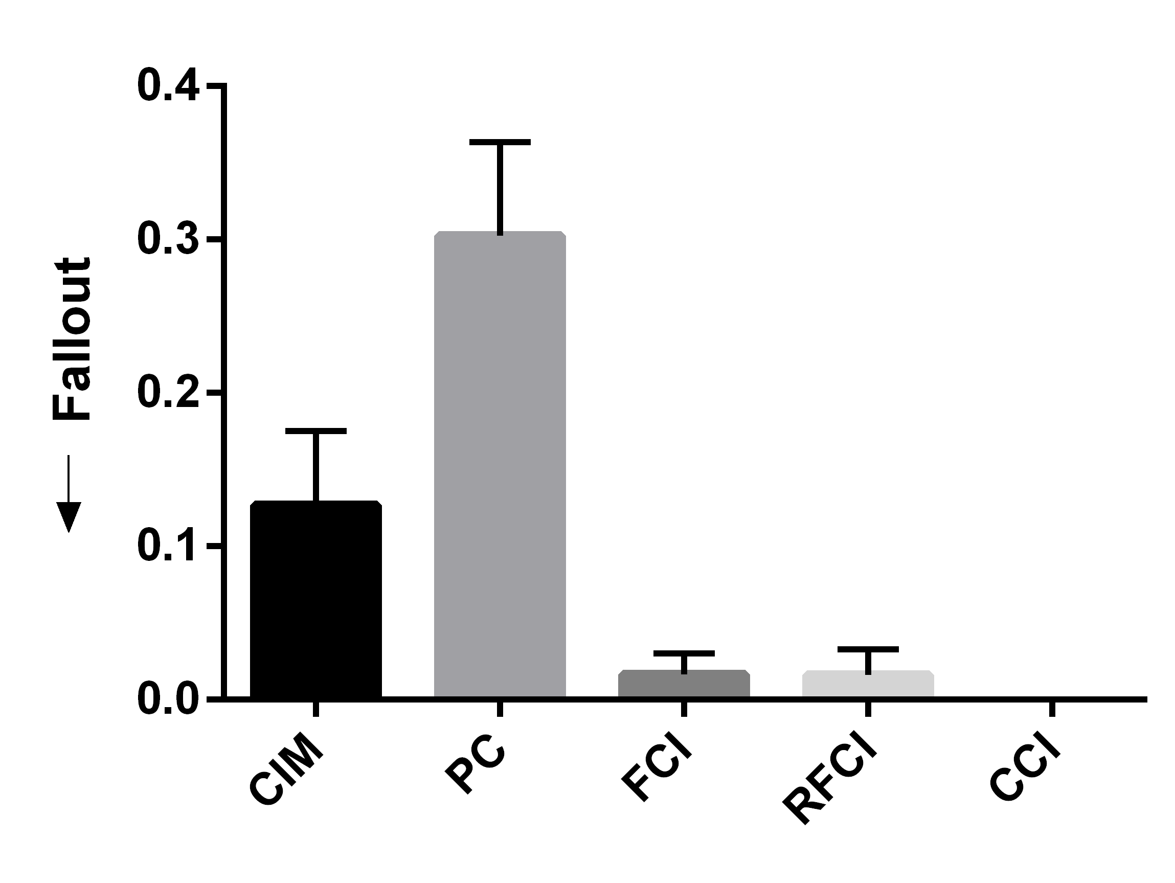 Figure 8
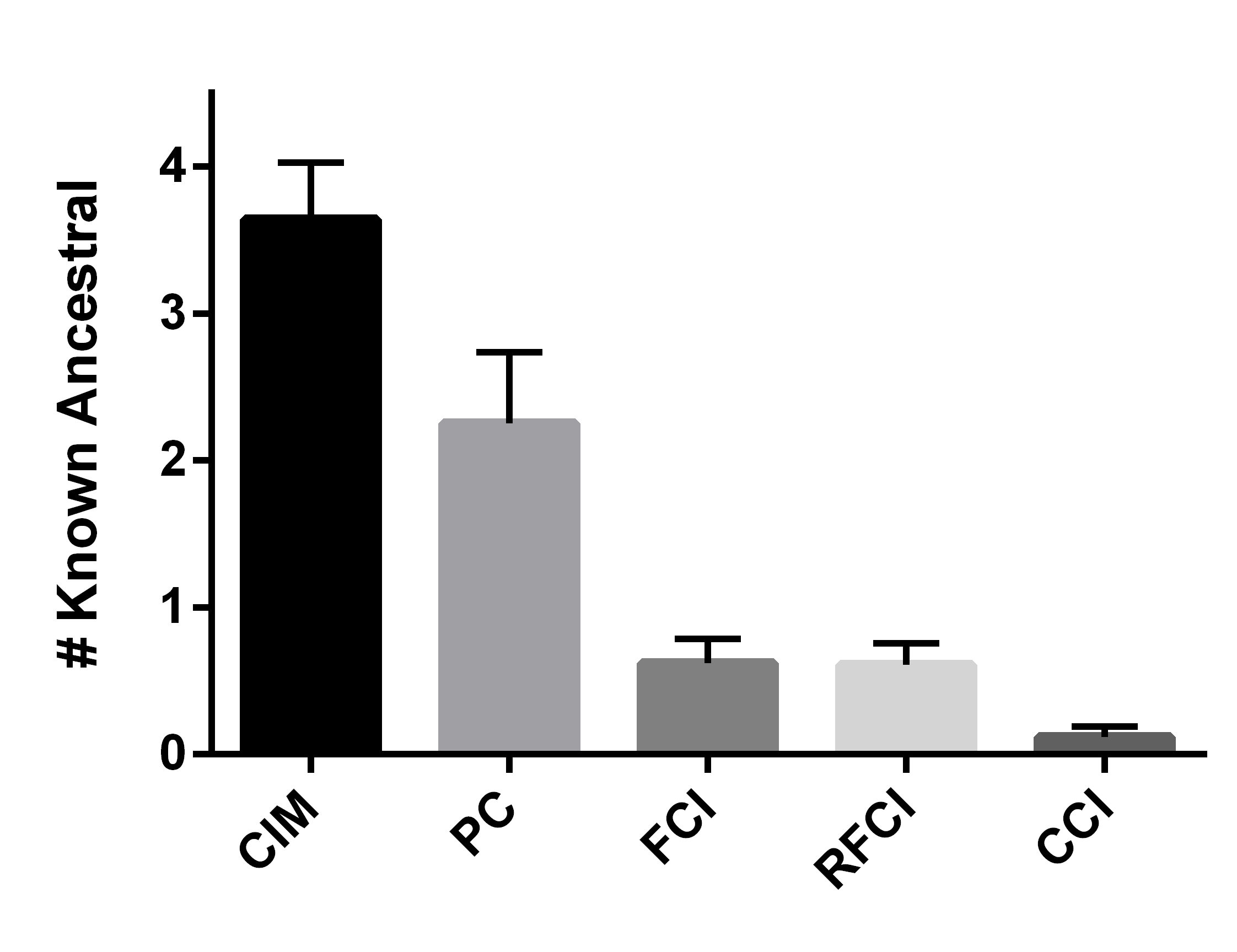 Figure 9
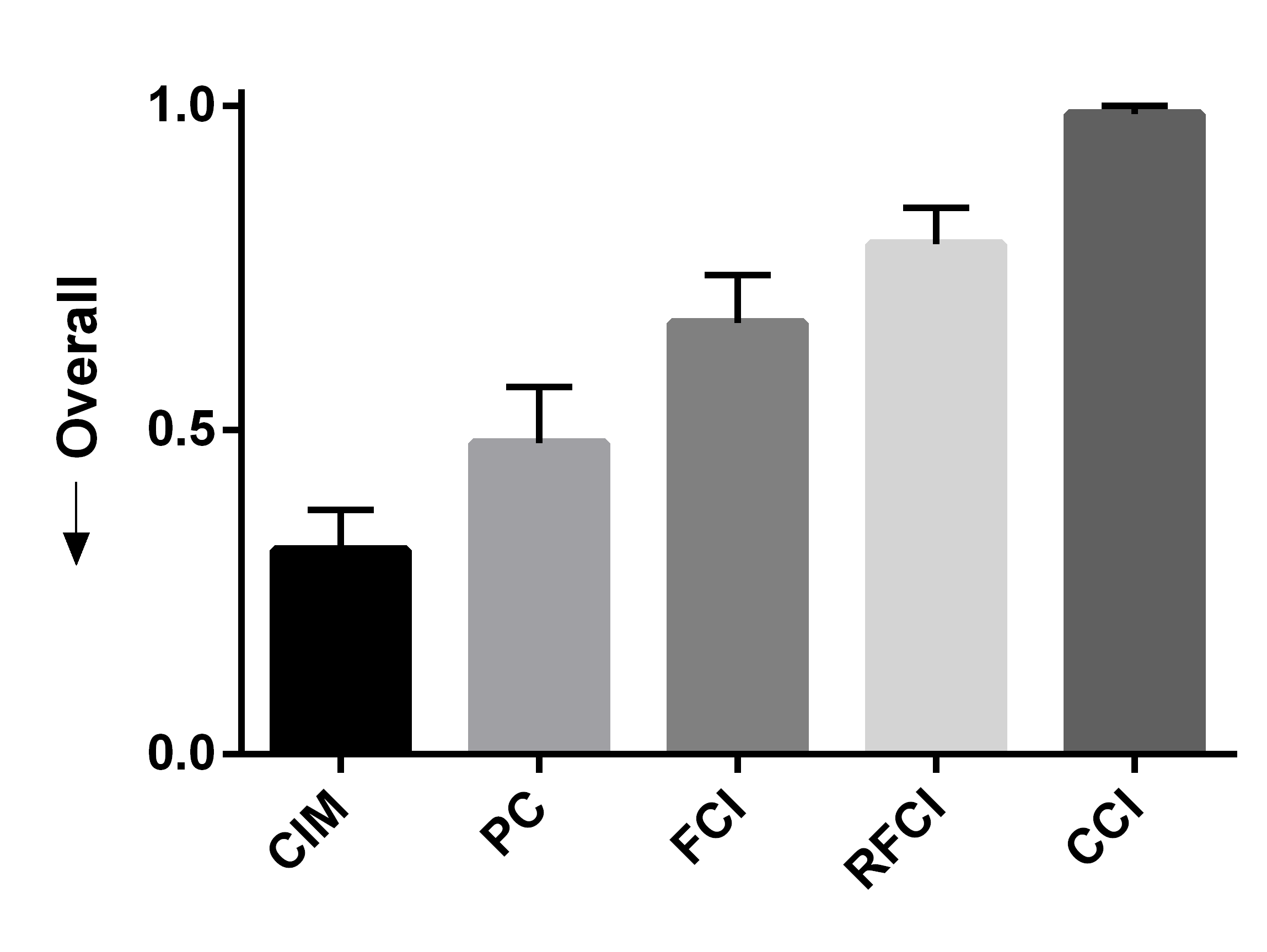 Figure 10
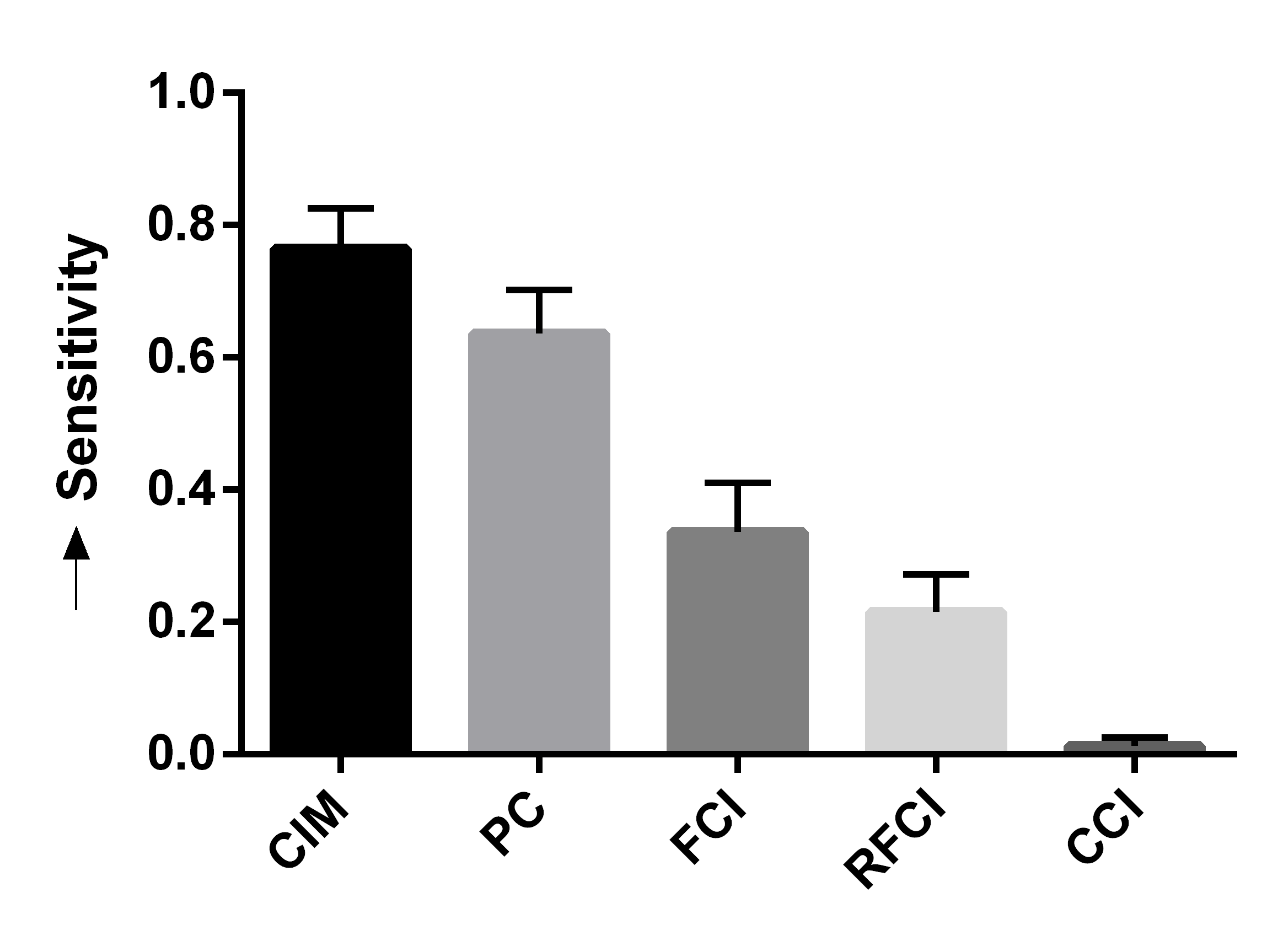 Figure 11
 Figure 12
| 0.21 | -0.20 | 1.29 |
| 0.68 | -0.47 | 7.30 |
| 1.05 | -0.19 | 4.33 |
| 0.72 | -1.40 | 0.10 |
| 0.13 | -0.56 | 2.91 |
| 0.31 | -1.01 | 5 | 0 | 1.29 | |
| 0.89 | -0.58 | 6 | 0 | 7.30 | |
| 1.11 | -0.79 | 2 | 1 | 4.33 | |
| 0.14 | -1.23 | 5 | 0 | 0.10 | |
| 0.21 | -0.20 | 4 | 1 | 2.91 | |
Peer Reviews
No public reviews on file for this paper yet. If you reviewed it on a platform where reviews are public (OpenReview, ICLR, NeurIPS, ICML), you can paste yours below so the community can read it here.
Videos
No videos yet. Explain this paper in a talk, walkthrough, or lecture? Add one.
Taxonomy
MethodsCausal inference
Causal Discovery with a Mixture of DAGs
Eric V. Strobl
Psychiatry & Behavioral Sciences
Vanderbilt University Medical Center
Tennessee, United States
Abstract
Causal processes in biomedicine may contain cycles, evolve over time or differ between populations. However, many graphical models cannot accommodate these conditions. We propose to model causation using a mixture of directed cyclic graphs (DAGs), where the joint distribution in a population follows a DAG at any single point in time but potentially different DAGs across time. We also introduce an algorithm called Causal Inference over Mixtures that uses longitudinal data to infer a graph summarizing the causal relations generated from a mixture of DAGs. Experiments demonstrate improved performance compared to prior approaches.
keywords:
Causal discovery, Longitudinal data, Directed acyclic graph, Mixture of DAGs
1 Introduction
Causal discovery refers to the process of inferring causation from data. Investigators usually perform causal discovery in biomedicine using randomized controlled trials (RCTs). However, RCTs can be impractical or unethical to perform. For example, scientists cannot randomly administer illicit substances or traumatize healthy subjects. Many investigators therefore experiment with animals knowing that the derived results may not directly apply to humans.
In this paper, we develop an algorithm that discovers causation directly from human observational data, or data collected without randomization. Denote the variables in an observational dataset by . We summarize the causal relations between variables in using a directed graph, where the directed edge with means that is a direct cause of . Similarly, is a cause of if there exists a directed path, or a sequence of directed edges, from to . We want to recover the directed graph as best as possible using the observational dataset.
Directed graphs in nature often contain feedback loops, or cycles, where causes and directly causes . For example, Figure 1 (a) depicts a portion of the thyroid system where denotes the thyroid stimulating hormone (TSH) and the T4 hormone (T4). TSH released from the thyroid gland regulates T4 hormone release, while T4 feeds back to inhibit TSH release. Cycles such as these abound in biomedicine, so we must develop algorithms that can accommodate them in order to accurately model causal processes.
We propose to model a potentially cyclic causal process using multiple directed acyclic graphs (DAGs), or graphs with directed edges but no cycles. The causal process is represented as a DAG at any single point in time, but the DAG may change across time to accommodate feedback. We illustrate the idea by decomposing the cycle in Figure 1 (a) into two DAGs: TSH T4 and T4 TSH. For each sample, TSH first causes T4 release at time point and then T4 inhibits TSH release at time point . We however can only measure each sample at a single point in time, so the observational dataset in Figure 1(a) contains some samples in blue when TSH causes T4 and others in grey when T4 causes TSH. If we do not observe the time variable , then the observational dataset arises from a mixture of DAGs where the mixing occurs over time: . We must infer the directed graph in Figure 1 (a) using the samples from and alone. In practice, we observe more than two random variables without color coding and mixing occurs over a subset of variables denoting entities such as time, gender, income and disease status. Figure 1(b) therefore depicts a more realistic dataset.
We also develop a method for recovering a directed graph summarizing the causal relations arising from a mixture of DAGs. We do so by first reviewing related work in Section 2. We then provide background in Section 3. Section 4 introduces the mixture of DAGs framework. In Section 5, we detail the algorithm called Causal Inference over Mixtures (CIM) to infer causal relations using longitudinal data. We then report experimental results in Section 6 highlighting the superiority of CIM compared to prior approaches on both real and synthetic datasets. We finally conclude the paper in Section 7. We delegate all proofs to the Appendix.
This paper improves upon a previous conference paper [1]. We made the following changes: (1) simplified exposition, (2) improved characterization of a mixture of DAGs, (3) corrected theoretical results, (4) an enhanced CIM algorithm, (5) experiments with better evaluation metrics. This report therefore provides more convincing material compared to the conference paper.
2 Related Work
Several algorithms perform causal discovery with cycles. Most of these methods assume stationarity, or a stable distribution over time and populations. The Fast Causal Inference (FCI) algorithm for example infers causal relations when cycles exist [2, 3]. The algorithm was initially developed for the acyclic case, but it can infer the acyclic portions of a cyclic graph by ignoring the independence relations within cycles. Other algorithms attempt to recover within-cycle causal relations. The Cyclic Causal Discovery (CCD) algorithm for instance works well when no selection bias or latent variables exist. The Cyclic Causal Inference (CCI) algorithm extends CCD to handle selection bias and latent variables, but both algorithms require linear or discrete variables for correctness [4, 5, 6].
Investigators have extended FCI, CCD and CCI with answer set programming (ASP). ASP algorithms allow the user to easily incorporate prior knowledge and infer causal relations more accurately. These methods however only apply to datasets with less than 10-20 variables due to scalability issues with a conventional laptop [7, 8].
Another set of methods focus on non-stationarity, but most of them require a single underlying directed graph [9, 10, 11, 12, 13]. Two methods exist for recovering causal processes with multiple graphs [14, 15], but they assume a mixture of parametric distributions. CIM improves upon all of these methods by allowing non-linearity, cycles, non-stationarity, non-parametric distributions, changing graphical structure, latent variables and selection bias.
3 Background
We now delve into the background material required to understand the proposed methodology.
3.1 Terminology
In addition to directed edges, we consider other edge types including: (bidirected), — (undirected), (partially directed), (partially undirected) and (nondirected). The edges contain three endpoint types: arrowheads, tails and circles. We say that two vertices and are adjacent if there exists an edge between the two vertices. We refer to the triple as a collider or v-structure, where each asterisk corresponds to an arbitrary endpoint type. A collider or v-structure is said to be unshielded when and are non-adjacent. The triple is conversely a triangle if and are adjacent. Unless stated otherwise, a path is a sequence of edges without repeated vertices. is an ancestor of if there exists a directed path from to or . We write when is an ancestor of in the graph . We also apply the definition of an ancestor to a set of vertices as follows:
[TABLE]
If , and are disjoint sets of vertices in , then and are said to be d-connected by in a directed graph if there exists a path between some vertex in and some vertex in such that, for any collider on , is an ancestor of and no non-collider on is in . We also say that and are d-separated by if they are not d-connected by . For shorthand, we write to denote d-separation and to denote d-connection. The set is more specifically called a minimal separating set if we have but , where denotes any proper subset of .
A mixed graph contains edges with only arrowheads or tails, while a partially oriented mixed graph may also include circles. We focus on mixed graphs that contain at most one edge between any two vertices. We can associate a mixed graph with a directed graph as follows. We first partition denoting observed, latent and selection variables, respectively. We then consider a graph over summarizing the ancestral relations in with the following endpoint interpretations: in if , and in if .
3.2 Probabilistic Interpretation
We associate a density to a DAG by requiring that the density factorize into the product of conditional densities of each variable given its parents:
[TABLE]
Any distribution which factorizes as above also satisfies the global Markov property w.r.t. where, if we have in , then and are conditionally independent given [16]. We denote the conditional independence (CI) as for short. We refer to the converse of the global Markov property as d-separation faithfulness. An algorithm is constraint-based if it utilizes CI testing to recover some aspects of as a consequence of the global Markov property and d-separation faithfulness.
4 Mixture of DAGs
We introduce the framework with univariate and then generalize to multivariate because the univariate case is simpler.
4.1 Univariate Case
We consider the set of vertices . We divide into three non-overlapping sets , and denoting observed, latent and selection variables, respectively. At each time point , we consider the joint density and assume that it factorizes according to a DAG over :
[TABLE]
where refers to for shorthand, the parent set of at time point . We analyze the following density:
[TABLE]
where . The above equation differs from Equation (1) for a single DAG; the parent set remains constant over time in Equation (1), but the parent set may vary over time in Equation (2).
Let correspond to all those variables in where , so that for all . We can then rewrite Equation (2):
[TABLE]
The left hand term corresponds to the stationary component and the right hand to the non-stationary component. We assume that we can sample from the mixture density :
[TABLE]
where mixing occurs over time in the integration if . We refer to the above equation as the mixture of DAGs framework.
4.2 Multivariate Case
We generalize the mixture of DAGs framework to a multivariate set of mutually independent mixture variables . For example, we may let , where denotes time and gender. Gender is instantiated independent of time, but the causal process can change over time and differ by gender. We may also observe gender but not observe time so that but . The set can therefore encompass a wide range of variables.
We consider the set of vertices instead of the original . We divide into three non-overlapping sets , and . We assume a joint density that factorizes according to a DAG over :
[TABLE]
where . The above equation mirrors Equation (2).
For each , let denote the largest set such that . This implies . We then rewrite Equation (4):
[TABLE]
so that is stationary over but non-stationary over . Setting and for and vice versa for recovers Equation (3). We finally sample from the mixture density :
[TABLE]
4.3 Global Markov Property
The factorization in Equation (5) implies certain CI relations. In this section, we will identify the CI relations by deriving a global Markov property similar to the traditional DAG case.
There exists a DAG for each instantiation of because is defined for all . Consider the collection consisting of all DAGs indexed by . The number of DAGs over is finite, so . Let denote the values of corresponding to any member of , and to those for . We can then rewrite Equation (5) as:
[TABLE]
where refers to the parents of in , and the children. If , then we use to more directly refer to the vertices corresponding to . We let .
We adopt the following procedure:
Plot each of the DAGs in adjacent to each other. 2. 2.
Combine the vertices into a single vertex for each . 3. 3.
Add additional directed edges so that the children of correspond to for each .
Denote the resultant graph as the mixture graph . If , then in due to step 2 above. We can read off the implied CI relations from by utilizing d-separation across groups of vertices rather than just singletons.
Theorem 1**.**
(Global Markov property) Let denote disjoint subsets of . If in , then .
We refer to the reverse direction as d-separation faithfulness with respect to . The result improves that of [17] (Appendix 8.3) and extends that of [18] when is partially observed, continuous or multivariate. We provide an example in Figure 2. Suppose indexes two DAGs. We plot the two DAGs next to each other in Figure 2 (a) and combine the vertices associated with as in Figure 2 (b). We have in the first DAG and in the second; however, we do not have the directed path in either DAG. We also have the relation , so implies per Theorem 1.
5 Causal Inference over Mixtures
5.1 Fused Graph
We construct a fused graph as follows. Create a vertex for every variable in . Draw a directed edge if and only if is a direct cause of in , so that may contain cycles. The fused graph is more intuitive than the mixture graph because summarizes cycles in one directed graph. We will utilize the global Markov property of in order to recover a mixed graph summarizing the ancestral relations in . For example, suppose we have the mixture graph drawn in Figure 3 (a). We consider a cycle involving and consider two slow causal relations: and . We thus have in the first DAG in , but is overwritten by this causal relation, so we do not observe . Likewise, we have in the second DAG, but is overwritten, so we do not observe . We therefore cannot observe causing in either DAG due to the two rate limiting steps even though causes in the cycle involving . Moreover, if we intervene on the value of , then cannot be overwritten in the second DAG, so we would observe causing . Now we have also drawn out in Figure 3 (b). is an ancestor of in even though is not an ancestor of in . Discovering thus allows us to infer cycles that are not present within but exist once the DAGs are combined in .
5.2 Strategy
We unfortunately cannot recover non-ancestral relations using a CI oracle alone (Appendix 8.4), but we can recover ancestral relations. We therefore rely on additional time information to orient arrowheads by utilizing longitudinal data, or data arising from a longitudinal density. We can partition the observed variables into sets or waves so that . We have the following definition:
Definition 1**.**
(Longitudinal density) A longitudinal density is a density that factorizes according to Equation (5) such that no variable in wave is an ancestor of a variable in wave and .
Causation proceeds forward in time, so no variable in wave can be an ancestor of a variable in wave .
If , then let and denote and , respectively. We write to mean those variables between waves and inclusive that are adjacent to in . We will specifically construct with the following adjacencies:
List 1**.**
*(Adjacency Interpretations)
If we have (with possibly ), then in for all and all . 2. 2.
If we do not have (with possibly ), then in for some between waves and inclusive.
The endpoints of have the following modified interpretations:
List 2**.**
*(Endpoint Interpretations)
If , then . 2. 2.
If , then .
The arrowheads do not take into account selection variables because we often cannot a priori specify whether a variable is an ancestor of in using either wave information or other prior knowledge in practice. We draw an example of in Figure 3 (a), its fused graph in Figure 3 (b) and the corresponding mixed graph in Figure 3 (c), where , , and .
5.3 Algorithm
We cannot apply an existing constraint-based algorithm like FCI on data arising from a mixture of DAGs and expect to recover a partially oriented (Appendix 8.5). We therefore propose a new algorithm called Causal Inference over Mixtures (CIM) which correctly recovers causal relations. We summarize the procedure in Algorithm 1.
The CIM algorithm works as follows. First, CIM runs a variant of PC-stable’s skeleton discovery procedure in order to discover adjacencies as well as minimal separating sets in Step 1 [19]. This step recovers the adjacencies with interpretations listed in List 1. The algorithm stores the minimal separating sets in the array Sep so that contains a minimal separating set of and , if such a set exists. CIM next adds arrowheads in Step 1 using wave information from a longitudinal dataset with the list . If we have with , then CIM orients because . We can orient additional arrowheads using other prior knowledge . Step 1 orients many arrowheads in practice, so long as we have at least two waves of data and repeated measurements.
For every triple with and non-adjacent, CIM then attempts to find a minimal separating set that contains in Step 1. These sets are important due to the following lemma which allows us to infer tails in Step 1:
Lemma 1**.**
Suppose in but for every . If , then .
CIM finally adds some additional tails in Step 1 due to transitivity of the tails. The algorithm has the same polynomial time complexity as PC-stable due to Step 1.
We now formally claim that Algorithm 1 is sound:
Theorem 2**.**
Suppose the longitudinal density factorizes according to Equation (5). Assume that all arrowheads deduced from are correct. Then, under d-separation faithfulness w.r.t. , the CIM algorithm returns the mixed graph partially oriented.
6 Experiments
We had two overarching goals: (1) evaluate the performance of CIM against other constraint-based algorithms using real data, and (2) determine if we can reconstruct the real data results using synthetic data sampled from a mixture of DAGs. We therefore utilized the setup described below.
6.1 Algorithms
We compared the following five constraint-based algorithms in recovering the ancestral and nonancestral relations in : CIM, PC, FCI, RFCI and CCI. We equipped all algorithms with a nonparametric CI test called GCM [20] and fixed across all experiments. We gave all algorithms the same wave information during skeleton discovery in order to orient arrowheads between the waves. The algorithms perform much worse without the additional knowledge.
6.1.1 Metrics
Let tails refer to positives and arrowheads to negatives. CIM only infers tails, so we cannot compute the number of true and false negatives. We can however compute the number of true positives and false positives.
We therefore evaluated the algorithms using sensitivity and fallout. The sensitivity is defined as , where refers to true positives and to positives. The fallout is defined as , where refers to false positives and to negatives. A tail in place of an arrowhead corresponds to a false positive.
The receiver operating characteristic (ROC) curve plots sensitivity against the fallout. Perfect accuracy corresponds to a sensitivity of one and a fallout of zero at the upper left hand corner of the ROC curve. Constraint-based algorithms do not output a continuous score required to compute the area under the ROC curve, but we can assess overall performance using the Euclidean distance from the upper left hand corner [21].
6.2 Real Data
6.2.1 Framingham Heart Study
We first evaluated the algorithms on real data. We considered the Framingham Heart Study, where investigators measured cardiovascular changes across time in residents of Framingham, Massachusetts [22]. The dataset contains three waves of data with 8 variables in each wave. We obtained 2019 samples after removing patients with missing values.
The dataset contains the following known direct causal relations: (1) number of cigarettes per day causes heart rate via cardiac nicotonic acetylcholine receptors [23, 24, 25]; (2) age causes systolic blood pressure due to increased large artery stiffness [26, 27]; (3) age causes cholesterol levels due to changes in cholesterol and lipoprotein metabolism [28]; (4) BMI causes number of cigarettes per day because smoking cigarettes is a common weight loss strategy [29, 30]; (5) systolic blood pressure causes diastolic blood pressure and vice versa by definition, because both quantities refer to pressure in the same arteries at different points in time. We can compute sensitivity using this information.
We summarize the results over 50 bootstrapped datasets in Figures 4 (a, b, c). We first evaluated sensitivity by running the algorithms using the full wave information. RFCI, FCI and CCI oriented few tails overall, so they obtained lower sensitivity scores (Figure 4 (a)). PC and CIM had similar sensitivities (t=-0.80, p=0.43). We next combined waves 2 and 3, so that the algorithms could incorrectly orient tails backwards in time. CIM made fewer errors than PC as indicated by a lower fallout (Figure 4 (b), t=-11.85, p=5.37E-16). FCI, RFCI and CCI also achieved low fallout scores, but they again did not orient many tails to begin with. CIM therefore obtained the best overall score when we combined sensitivity and fallout (Figure 4 (c), t=-5.60, p=9.70E-7). We conclude that both CIM and PC orient many tails, but CIM makes fewer errors as evidenced by its high sensitivity and low fallout. We therefore prefer CIM in this dataset.
6.2.2 Sequenced Treatment Alternatives to Relieve Depression Trial
We next analyzed Level 1 of the Sequenced Treatment Alternatives to Relieve Depression (STAR∗D) trial [31]. Investigators gave patients an antidepressant called citalopram and then tracked their depressive symptoms using a standardized questionnaire called QIDS-SR-16. We analyzed the 9 QIDS-SR-16 sub-scores measuring components of depression at weeks 0, 2 and 4. We also included age and gender in the first wave. The dataset contains 2043 subjects after removing subjects with missing values.
The 9 QIDS-SR-16 subscores include sleep, mood, appetite, concentration, self-esteem, thoughts of death, interest, energy and psychomotor changes. We asked a psychiatrist to identify direct ground truth causal relations among the subscores before we ran the experiments. The ground truth includes: (1) sleep causes mood [32]; (2) energy causes psychomotor changes; (3) appetite causes energy; (4, 5) mood causes appetite and self-esteem [33]; (6) psychomotor changes cause concentration; (7, 8) mood and self-esteem cause thoughts of death [34].
We summarize the sensitivity, fallout and overall performance over 50 bootstrapped datasets in Figures 4 (d, e, f). CIM achieved higher sensitivity than all other algorithms (Figure 4 (d), t=5.66, p=7.86E-7). CIM also had a smaller fallout score compared to PC (Figure 4 (e), t=-19.19, p2.20E-16). CIM therefore obtained the highest overall score compared to the other algorithms (Figure 4 (f), t=-14.95, p2.20E-16). These results corroborate the superiority of CIM in a second real dataset.
6.3 Synthetic Data
We next sampled from a mixture of DAGs to see if we could replicate the real data results. We specifically instantiated a linear DAG with an expected neighborhood size of 2, vertices and linear coefficients drawn from Uniform(). We then uniformly instantiated to 15 binary variables for and block randomized the edges in the DAG to each element of . We assigned the first 8 variables to wave 1, the second 8 to wave 2, and the third 8 to wave 3. We added a directed edge from the variable in wave 1 to the variable in wave 2, and similarly added the directed edges from wave 2 to wave 3 in order to model self-loops. We randomly selected a set of 0-2 latent common causes without replacement from , which we placed in in addition to the variables in . We then selected a set of 0-2 selection variables without replacement from the set .
We uniformly instantiating the mixing probabilities and for each . We then generated 2000 samples as follows. For each sample, we drew an instantiation according to and created a graph containing the union of the edges associated with those elements in equal to one. We then sampled the resultant DAG using a multivariate Gaussian distribution. We finally removed the latent variables and introduced selection bias by removing the bottom percentile for each selection variable, with chosen uniformly between 10 and 50.
We report the results in Figures 4 (g, h, i) after repeating the above process 50 times. We computed the sensitivity and fallout using the ground truth in waves 2 and 3. CIM achieved the highest sensitivity (Figure 4 (g), t=3.71, p=5.35E-4). PC obtained the second highest sensitivity, but CIM had a lower fallout than PC (Figure 4 (h), t=-4.63,p=2.72E-5). CIM ultimately achieved the best overall score (Figure 4 (i), t=-3.78,p=4.37E-4). We conclude that the synthetic data results mimic those seen with the real data.
7 Conclusion
We proposed to model causal processes in biomedicine using a mixture of DAGs to accommodate non-stationary distributions and cycles. We then introduced a constraint-based algorithm called CIM to infer causal relations from data even with latent variables and selection bias. The CIM algorithm outperforms existing constraint-based algorithms across multiple metrics and datasets. CIM thus advances the state of the art in causal discovery from biomedical data.
8 Appendix
8.1 Proofs
Theorem 1.
Let denote disjoint subsets of . If in , then .
Proof.
We first consider the moral graph of . Let denote the moral graph of , the smallest ancestral set of in such that, if , then . We then consider a partition of the vertices so that , , and , and are disjoint sets of vertices. We require that and be separated by in ; in other words, there does not exist an undirected path between and that is active given .
We now construct such a partition . First set to and to . We have in if and only if and are separated by in (Lemma 2 in [16]). and are therefore separated by in at the moment. Now consider the set of vertices We will put subsets of into either or . We have two situations for each .
In , there does not exist an undirected path between and or an undirected path between and (or both) that is active given . More specifically:
- (a)
If there does not exist an undirected path between and that is active given , but such a path exists between and , then include into . 2. (b)
If there does not exist an undirected path between and that is active given , but such a path exists between and , then include into . 3. (c)
If there does not exist an undirected path between and that is active given and there likewise does not exist such a path between and , then include into . 2. 2.
In , there exists an undirected path between and and an undirected path between and that are both active given . We have two cases:
- (a)
There exists an undirected path between and and an undirected path between and that are both active given . But this implies that and are connected given in via - a contradiction. 2. (b)
There exists an undirected path between and and an undirected path between ( and that are both active given - denote these paths by and , respectively. Note that there does not exist an undirected path between and and an undirected path between and that are both active given per the argument in (a). We have two cases:
- i.
There does not exist a descendant of on . Then must be confined to the sub-graph in . But then an analogous undirected path must be active in the sub-graph - a contradiction. A similar argument also applies to . 2. ii.
Let denote all members of that have a descendant on . We will construct an active path between and in for a contradiction. We construct a path from in using the corresponding vertices on in until we encounter the first child of , denoted by . Consider the collection , for some , whose concatenation connects and given in - a contradiction. A similar argument also applies to .
We have exhausted all possibilities and therefore conclude that there cannot exist an undirected path between and and an undirected path between and that are both active given .
We have constructed a disjoint partition of vertices such that . Moreover, and are separated given in because, if an active path exists between and given , this implies the contradiction that there also exists an active path between and given .
We may then consider all of the cliques in corresponding to each vertex and its married parents. Denote this set of cliques as . Also let denote the set of cliques in that have non-empty intersection with . Because and are separated given , the vertices and are also non-adjacent in ; this implies that no clique in can contain a member of . We also have for all .
Consider an arbitrary graph . We can write:
[TABLE]
where is a placeholder for some non-negative function for . Let and . Also let denote the sub-sets of the sets in corresponding to - likewise for . We then proceed by integrating out :
[TABLE]
where when and when . We then finalize the integration:
[TABLE]
The third equality follows because by construction. The conclusion follows by the last equality. ∎
Lemma 1.
Suppose in but for every . If , then .
Proof.
We invoke Lemma 15 in [4] by setting , , , and in that paper. We can then conclude that . Moreover, if , then by construction of . ∎
Theorem 2.
Suppose the longitudinal density factorizes according to Equation (5). Assume that all arrowheads deduced from are correct. Then, under d-separation faithfulness w.r.t. , the CIM algorithm returns the mixed graph partially oriented.
Proof.
Under d-separation faithfulness w.r.t. , CI and d-separation w.r.t. are equivalent by Theorem 1, so we can refer to them interchangeably. Algorithm 2 finds the adjacencies in List 1 because we must always have in Step 2 of Algorithm 2. Step 1 discovers the correct tails by Lemma 1. Step 1 follows directly by transitivity of the tails. ∎
8.2 Skeleton Discovery
We summarize CIM’s skeleton discovery procedure in Algorithm 2. The algorithm mimics PC-stable’s skeleton discovery procedure, but it incorporates wave information in the adjacency sets.
8.3 Comparison to Previous Global Markov Property
Spirtes [17] also characterized the global Markov property across a mixture of DAGs using . The fused graph however implies less CI relations than as illustrated in Figure 2. We have drawn in Figure 2 (c). and are d-connected in even though and are d-separated in in Figure 2 (b). We have established an instance where the mixture graph implies strictly more independence relations than the fused graph.
The mixture graph in fact always implies at least the same number of CI relations as the fused graph:
Proposition 1**.**
Let denote disjoint subsets of . If in , then in .
Proof.
We create copies of and plot them adjacent to each other. Denote the resultant graph as . As a result, we have in if and only if in . Create a new graph as follows. First set equal to . Then remove from and place instead. Set equal to for each . Denote the resultant graph as .
We will show that in implies in . Consider any active path between and given in . Denote the moral graph of by . Consider an active path between and given in . We can replace an arbitrary vertex on with on . Repeating this process for every vertex on creates a non-simple path (i.e. with potentially repeated vertices) between and that does not contain any member of . There thus exists a simple path without repeated vertices between and that does not contain any member of in . Hence in by Lemma 2 in [16].
Note that all of the edges in are contained within . The conclusion follows because we may write in implies in , which implies in , which implies in .
∎
is thus superior to because (1) implies at least as many CI relations as , and (2) implies strictly more CI relations in some cases.
8.4 Negative Result
We cannot infer arrowheads with a CI oracle alone:
Proposition 2**.**
There exist mother and fused graph pairs and such that and , but in if and only if in for any and .
Proof.
Assume . Let and refer to the set of DAGs associated with and , respectively. Choose arbitrarily and set equal to . If , then add a second copy of the DAG into . Add one new latent variable into each DAG in as follows. For all but the last DAG, draw the directed edge . For the last DAG, draw . Next, introduce a new latent common cause for and into every DAG in . The new paths do not introduce a d-connecting path between the observed vertices in any of the DAGs in . As a result, in if and only if in , but with the directed path . ∎
8.5 Failure of Other Constraint-Based Methods
We cannot apply an existing constraint-based algorithm on data arising from a mixture of DAGs and recover a partially oriented . For example, FCI and CCI can make incorrect inferences if contains more than one DAG. Consider the mixture graph in Figure 5 (a), where all variables lie in the same wave. is an ancestor of in drawn in Figure 5 (b), but we have in , so and are independent by Theorem 1. FCI and CCI therefore infer the incorrect collider in during v-structure discovery. We thus require an alternative algorithm to correctly recover a partially oriented .
The reference list from the paper itself. Each links out to its DOI / PubMed record.
- 1Strobl [2019] E. V. Strobl, Improved causal discovery from longitudinal data using a mixture of dags, in: T. D. Le, J. Li, K. Zhang, E. K. P. Cui, A. Hyvärinen (Eds.), Proceedings of Machine Learning Research, volume 104 of Proceedings of Machine Learning Research , PMLR, Anchorage, Alaska, USA, 2019, pp. 100–133. URL: http://proceedings.mlr.press/v 104/strobl 19a.html .
- 2Spirtes et al. [2000] P. Spirtes, C. Glymour, R. Scheines, Causation, Prediction, and Search, 2nd ed., MIT press, 2000.
- 3Zhang [2008] J. Zhang, On the completeness of orientation rules for causal discovery in the presence of latent confounders and selection bias, Artif. Intell. 172 (2008) 1873–1896. URL: http://dx.doi.org/10.1016/j.artint.2008.08.001 . doi: 10.1016/j.artint.2008.08.001 . · doi ↗
- 4Strobl [2018] E. V. Strobl, A constraint-based algorithm for causal discovery with cycles, latent variables and selection bias, International Journal of Data Science and Analytics (2018). URL: https://doi.org/10.1007/s 41060-018-0158-2 . doi: 10.1007/s 41060-018-0158-2 . · doi ↗
- 5Forré and Mooij [2017] P. Forré, J. M. Mooij, Markov properties for graphical models with cycles and latent variables, ar Xiv.org preprint ar Xiv:1710.08775 [math.ST] (2017). URL: https://arxiv.org/abs/1710.08775 .
- 6Forré and Mooij [2018] P. Forré, J. M. Mooij, Constraint-based causal discovery for non-linear structural causal models with cycles and latent confounders, in: Proceedings of the 34th Annual Conference on Uncertainty in Artificial Intelligence (UAI-18), 2018.
- 7Hyttinen et al. [2013] A. Hyttinen, P. O. Hoyer, F. Eberhardt, M. Järvisalo, Discovering cyclic causal models with latent variables: A general sat-based procedure, in: Proceedings of the Twenty-Ninth Conference on Uncertainty in Artificial Intelligence, UAI 2013, Bellevue, WA, USA, August 11-15, 2013. URL: https://dslpitt.org/uai/display Article Details.jsp?mmnu=1&smnu=2&article_id=2391&proceeding_id=29 .
- 8Hyttinen et al. [2014] A. Hyttinen, F. Eberhardt, M. Järvisalo, Constraint-based causal discovery: Conflict resolution with answer set programming, in: Proceedings of the Thirtieth Conference on Uncertainty in Artificial Intelligence, UAI’14, AUAI Press, Arlington, Virginia, United States, 2014, pp. 340–349. URL: http://dl.acm.org/citation.cfm?id=3020751.3020787 .