Separable Effects for Causal Inference in the Presence of Competing Events
Mats J. Stensrud, Jessica G. Young, Vanessa Didelez, James M. Robins,, Miguel A. Hern\'an

TL;DR
This paper introduces separable effects to clarify causal relationships in time-to-event studies with competing risks, enabling more precise effect estimation without cross-world assumptions.
Contribution
It proposes a novel framework for defining and identifying causal effects in the presence of competing events, avoiding cross-world contrasts and hypothetical interventions.
Findings
Separable effects can be identified under the assumption of treatment decomposition.
Application to prostate cancer trial demonstrates practical utility.
Distinct causal pathways for treatment effects are elucidated.
Abstract
In time-to-event settings, the presence of competing events complicates the definition of causal effects. Here we propose the new separable effects to study the causal effect of a treatment on an event of interest. The separable direct effect is the treatment effect on the event of interest not mediated by its effect on the competing event. The separable indirect effect is the treatment effect on the event of interest only through its effect on the competing event. Similar to Robins and Richardson's extended graphical approach for mediation analysis, the separable effects can only be identified under the assumption that the treatment can be decomposed into two distinct components that exert their effects through distinct causal pathways. Unlike existing definitions of causal effects in the presence of competing events, our estimands do not require cross-world contrasts or hypothetical…
Click any figure to enlarge with its caption.
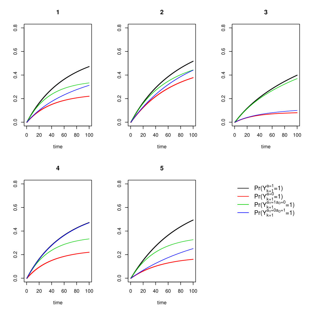 Figure 1
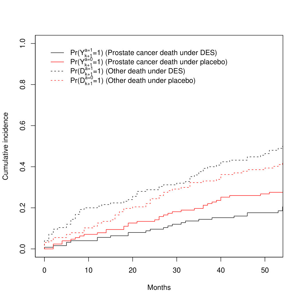 Figure 2
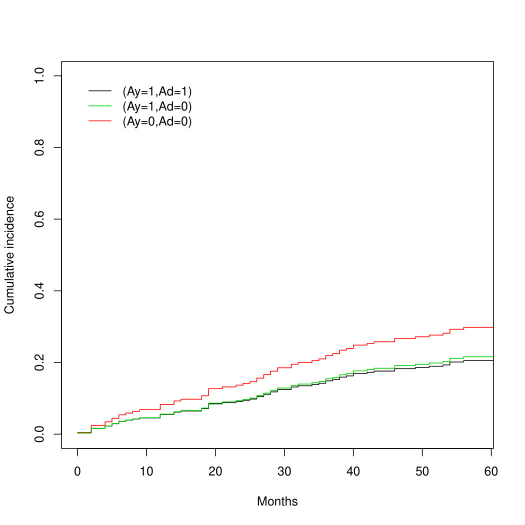 Figure 3
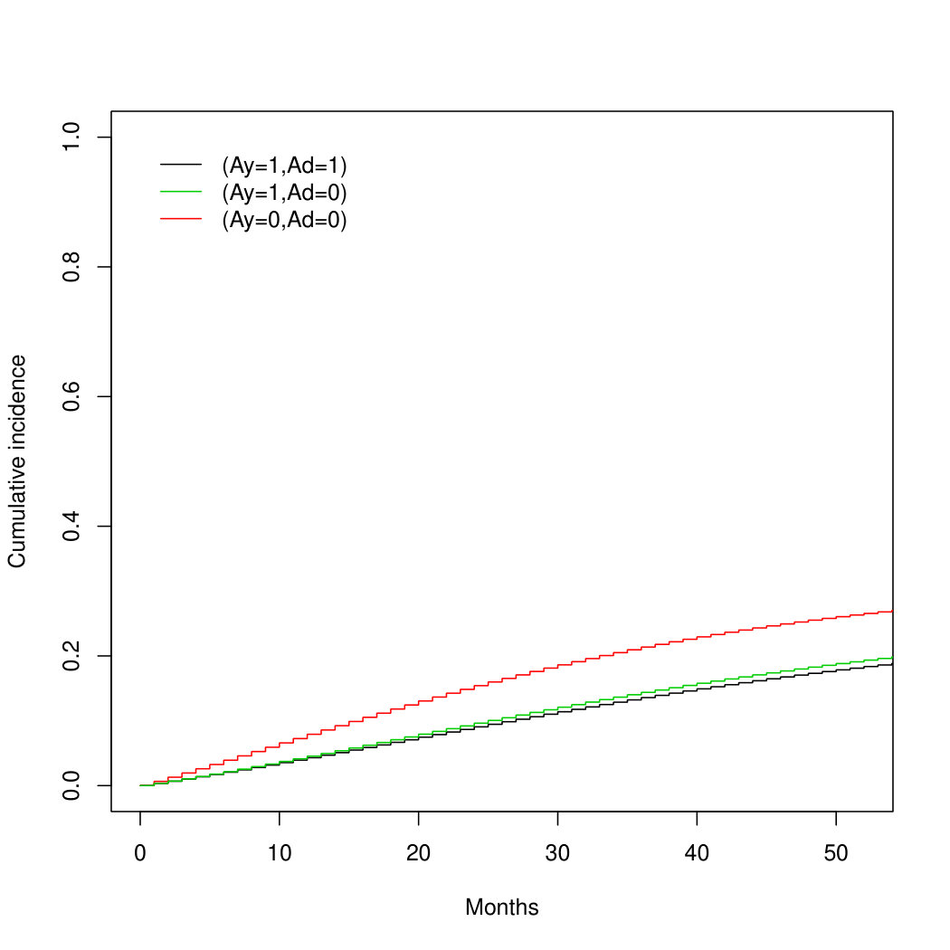 Figure 4
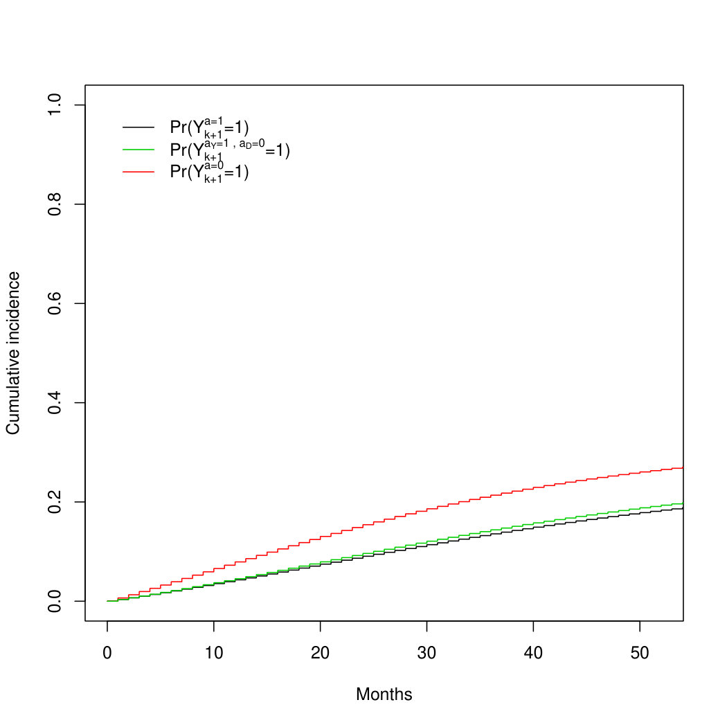 Figure 5
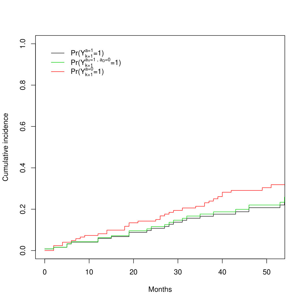 Figure 6
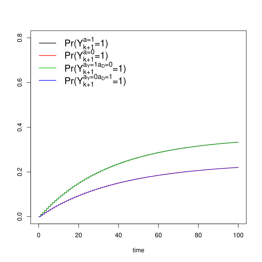 Figure 7
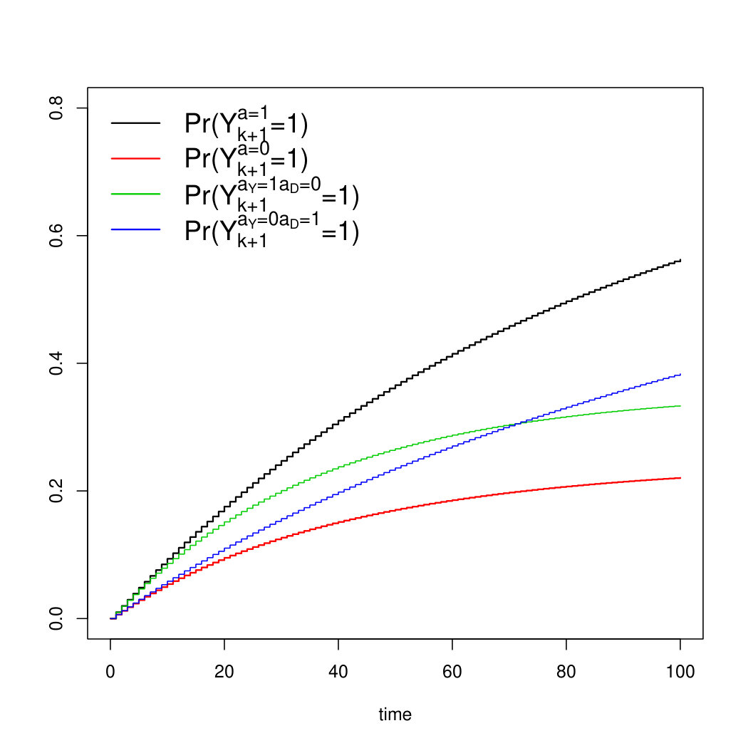 Figure 8
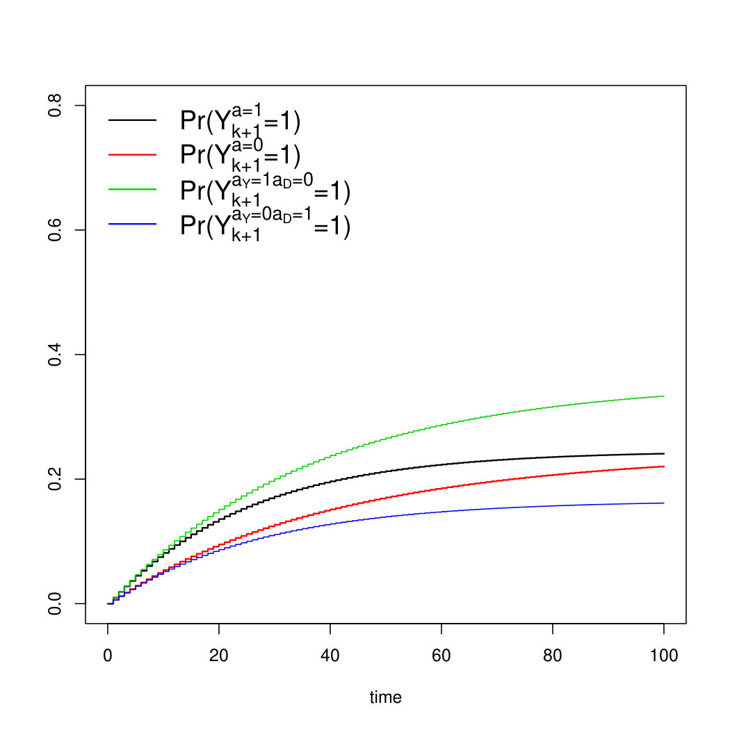 Figure 9
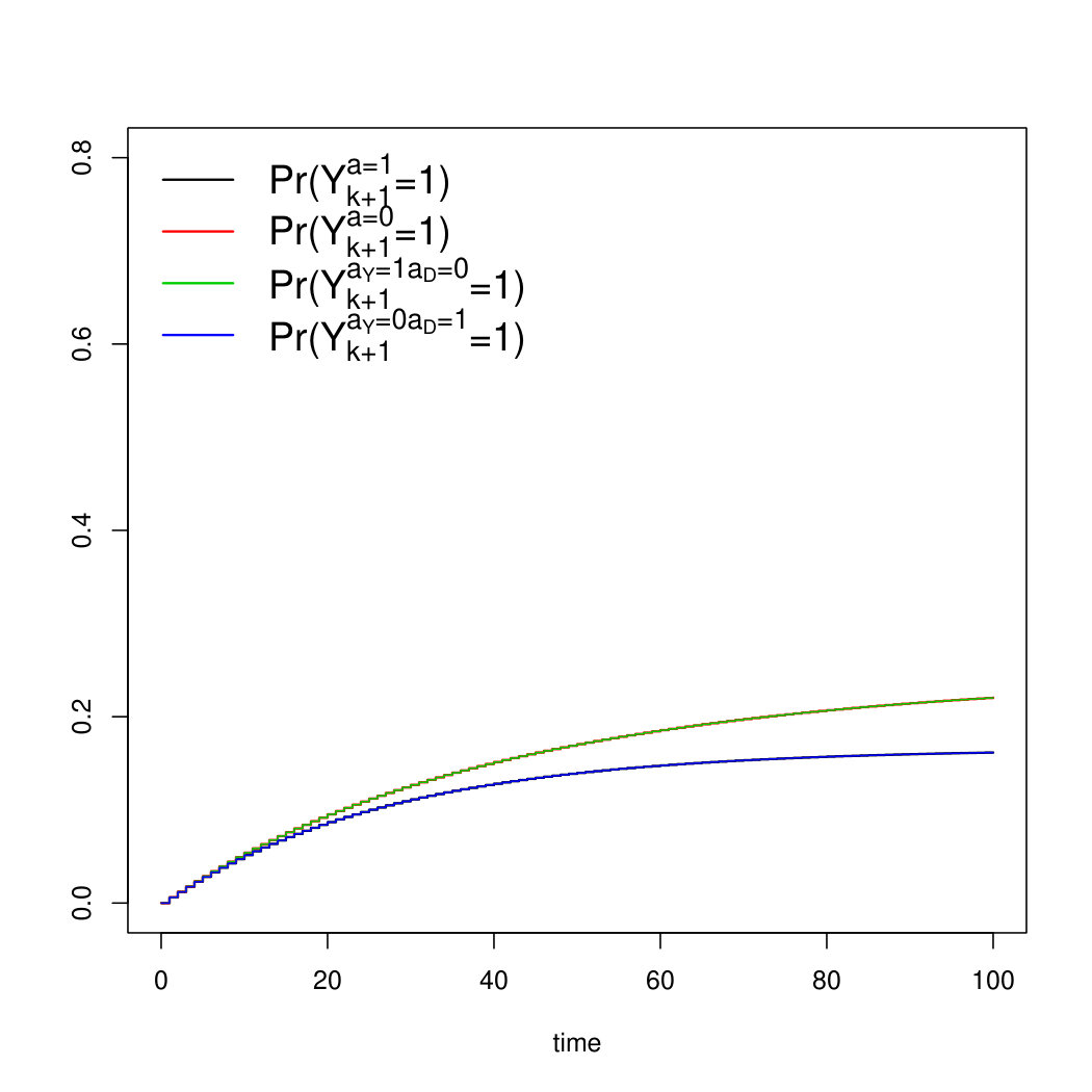 Figure 10
 Figure 11
| Estimand | G-formula estimate (95%CI) | IP weighted estimate (95%CI) |
|---|---|---|
| 0.14 (0.08-0.20) | 0.17 (0.10, 0.24) | |
| 0.15 (0.09-0.21) | 0.18 (0.10, 0.26) | |
| 0.21 (0.15-0.28) | 0.23 (0.17, 0.35) |
| Scenario | |||||||||
|---|---|---|---|---|---|---|---|---|---|
| 1 | 0.01 | 0 | 10 | 5 | 0.03 | 0 | 0 | 5 | |
| 2 | 0.01 | 0 | 0 | 5 | 0.03 | 0 | 5 | 5 | |
| 3 | 0.01 | 0 | 10 | 5 | 0.03 | 0 | 5 | 5 | |
| 4 | 0.01 | 0 | 10 | 5 | 0.03 | 0 | -5 | 5 |
| Treatment | Outcomes at in | Outcomes at in |
|---|---|---|
| or |
| Scenario | ||||||||||||||||
|---|---|---|---|---|---|---|---|---|---|---|---|---|---|---|---|---|
| 1 | 0.01 | 0 | 10 | 0 | 5 | 0 | 0 | 0 | 0.03 | 0 | 0 | -2 | 5 | 0 | 0 | 0 |
| 2 | 0.01 | 0 | 10 | 0 | -2 | 5 | 0 | 0 | 0.03 | 0 | 0 | -2 | 5 | -2 | 0 | 0 |
| 3 | 0.01 | 0 | 10 | 0 | 5 | -10 | 5 | 0 | 0.03 | 0 | 0 | -2 | 5 | -10 | 0 | 0 |
| 4 | 0.01 | 0 | 10 | 5 | 5 | 0 | 0 | 0 | 0.03 | 0 | 0 | -2 | 5 | 0 | 0 | 0 |
| 5 | 0.01 | 0 | 10 | 0 | -10 | 0 | 0 | 0 | 0.03 | 0 | 0 | -2 | 0 | 0 | 0 | 0 |
| Parameter | Estimator | |||
|---|---|---|---|---|
| g-formula | 0.95 | 0.94 | 0.93 | |
| non-parametric | 0.95 | 0.94 | 0.95 | |
| g-formula | 0.94 | 0.93 | 0.92 | |
| non-parametric | 0.94 | 0.95 | 0.95 | |
| g-formula | 0.95 | 0.96 | 0.94 | |
| 0.94 | 0.95 | 0.95 | ||
| 0.96 | 0.95 | 0.95 | ||
| g-formula | 0.93 | 0.93 | 0.94 | |
| 0.92 | 0.90 | 0.95 | ||
| 0.94 | 0.94 | 0.92 | ||
| Parameter | Estimator | |||
|---|---|---|---|---|
| g-formula | 0.91 | 0.92 | 0.91 | |
| non-parametric | 0.95 | 0.96 | 0.93 | |
| g-formula | 0.94 | 0.94 | 0.93 | |
| non-parametric | 0.93 | 0.93 | 0.93 | |
| g-formula | 0.96 | 0.94 | 0.91 | |
| 0.93 | 0.95 | 0.93 | ||
| 0.91 | 0.92 | 0.88 | ||
| g-formula | 0.94 | 0.93 | 0.93 | |
| 0.90 | 0.91 | 0.93 | ||
| 0.93 | 0.94 | 0.94 | ||
| Parameter | Estimator | |||
|---|---|---|---|---|
| g-formula | 0.93 | 0.95 | 0.91 | |
| non-parametric | 0.93 | 0.93 | 0.94 | |
| g-formula | 0.93 | 0.86 | 0.48 | |
| non-parametric | 0.94 | 0.93 | 0.94 | |
| g-formula | 0.93 | 0.94 | 0.93 | |
| 0.94 | 0.94 | 0.93 | ||
| 0.91 | 0.72 | 0.56 | ||
| g-formula | 0.82 | 0.74 | 0.45 | |
| 0.95 | 0.95 | 0.94 | ||
| 0.84 | 0.72 | 0.33 | ||
| Parameter | Estimator | |||
|---|---|---|---|---|
| g-formula | 0.96 | 0.94 | 0.93 | |
| non-parametric | 0.95 | 0.94 | 0.94 | |
| g-formula | 0.93 | 0.93 | 0.92 | |
| non-parametric | 0.93 | 0.93 | 0.95 | |
| g-formula | 0.96 | 0.97 | 0.94 | |
| 0.94 | 0.96 | 0.94 | ||
| 0.97 | 0.96 | 0.96 | ||
| g-formula | 0.05 | 0.05 | 0.07 | |
| 0.31 | 0.26 | 0.34 | ||
| 0.05 | 0.04 | 0.12 | ||
| Parameter | Estimator | |||
|---|---|---|---|---|
| g-formula | 0.95 | 0.94 | 0.94 | |
| non-parametric | 0.95 | 0.95 | 0.95 | |
| g-formula | 0.94 | 0.94 | 0.93 | |
| non-parametric | 0.95 | 0.94 | 0.94 | |
| g-formula | 0.96 | 0.95 | 0.94 | |
| 0.97 | 0.96 | 0.95 | ||
| 0.95 | 0.95 | 0.94 | ||
| g-formula | 0.93 | 0.94 | 0.94 | |
| 0.94 | 0.93 | 0.94 | ||
| 0.94 | 0.94 | 0.94 | ||
Peer Reviews
No public reviews on file for this paper yet. If you reviewed it on a platform where reviews are public (OpenReview, ICLR, NeurIPS, ICML), you can paste yours below so the community can read it here.
Videos
No videos yet. Explain this paper in a talk, walkthrough, or lecture? Add one.
Taxonomy
TopicsAdvanced Causal Inference Techniques · Bayesian Modeling and Causal Inference · Qualitative Comparative Analysis Research
Separable Effects for Causal Inference in the Presence of Competing Events
Mats J. Stensrud1,2, Jessica G. Young3, Vanessa Didelez4,5,James M. Robins1,6, Miguel A. Hernán1,6,7
1 Department of Epidemiology, Harvard T. H. Chan School of Public Health, USA
2Department of Biostatistics, University of Oslo, Norway
3 Department of Population Medicine, Harvard Medical School and Harvard Pilgrim Health Care Institute, USA
4 Leibniz Institute for Prevention Research and Epidemiology – BIPS, Germany
5 Faculty of Mathematics / Computer Science, University of Bremen, Germany
6 Department of Biostatistics, Harvard T. H. Chan School of Public Health, USA
7 Harvard-MIT Division of Health Sciences and Technology, USA
Abstract.
In time-to-event settings, the presence of competing events complicates the definition of causal effects. Here we propose the new separable effects to study the causal effect of a treatment on an event of interest. The separable direct effect is the treatment effect on the event of interest not mediated by its effect on the competing event. The separable indirect effect is the treatment effect on the event of interest only through its effect on the competing event. Similar to Robins and Richardson’s extended graphical approach for mediation analysis, the separable effects can only be identified under the assumption that the treatment can be decomposed into two distinct components that exert their effects through distinct causal pathways. Unlike existing definitions of causal effects in the presence of competing events, our estimands do not require cross-world contrasts or hypothetical interventions to prevent death. As an illustration, we apply our approach to a randomized clinical trial on estrogen therapy in individuals with prostate cancer.
1. Introduction
A competing event is any event that makes it impossible for the event of interest to occur. For example, consider a randomized trial to estimate the effect of a new treatment on the 3-year risk of prostate cancer in which 1000 individuals with prostate cancer were assigned to the treatment and 1000 to placebo. All participants adhered to the protocol and remained under follow-up. After 3 years, 100 individuals in the treatment arm and 200 in the placebo arm died of prostate cancer. Also, 150 individuals in the treatment arm and 50 in the placebo arm died of other causes (e.g., cardiovascular disease). Death from cardiovascular disease is a competing event for death from prostate cancer: individuals who die of cardiovascular disease cannot subsequently die of prostate cancer. When competing events are present, several causal estimands may be considered to define the causal effect of treatment on a time-to-event outcome [1].
Consider first the total treatment effect [1] defined by the contrast of the cumulative incidence (risk) [2, 3] of the event of interest under different treatment values. In our example, the total treatment effect on death from prostate cancer is the contrast of the cumulative incidence of death from prostate cancer under treatment, consistently estimated by , and under placebo, consistently estimated by . Therefore, the estimate of the total treatment effect on the additive scale is , which indicates that treatment reduced the risk of death from prostate cancer.
However, in our trial, the interpretation of the total treatment effect on the event of interest is difficult because the treatment also increased the risk of the competing event. The estimate of the total effect of treatment on the competing event is on the additive scale. Thus, it is possible that the beneficial effect of treatment on death from prostate cancer is simply a consequence of the harmful effect of treatment on death from other causes: when more people die from other causes, fewer people can die from prostate cancer. Note that this problem of interpretation cannot be solved by considering contrasts of hazard functions, such as cause-specific and subdistribution hazards, because these estimands are defined conditional on a post-treatment event (survival) and therefore do not generally have a causal interpretation [1, 4].
One way to deal with this problem is to consider a second causal estimand on the risk scale: the (controlled) direct effect of treatment on the event of interest had competing events been eliminated. This estimand corresponds to defining the competing events as censoring events [1], and is sometimes denoted the marginal (net) distribution function. Unlike the total effect, identification of the controlled direct effect requires untestable assumptions even in an ideal randomized trial with perfect adherence and no loss to follow-up [1]. Also, this causal estimand often introduces a new conceptual challenge: the direct effect is not sufficiently well-defined because there is no scientific agreement as to which hypothetical intervention, if any, would eliminate the competing events [5]. For example, in our prostate cancer trial, no intervention has ever been proposed that can prevent all deaths from causes other than prostate cancer. As a byproduct of the ill-defined intervention to prevent competing events, effect estimates cannot be empirically verified – not even in principle – in a randomized experiment.
A third causal estimand is the survivor average causal effect (SACE) [6], which is the total treatment effect (on the risk scale) in the principal stratum of patients who would never experience the competing event under either level of treatment [1, 6, 7]. Unlike the total effect, the presence of competing events is not a problem when interpreting the SACE, because the SACE is restricted to subjects who do not experience competing events. However, identification of the SACE requires strong untestable assumptions, e.g. about cross-world counterfactuals, even in a perfectly executed trial. Also, the SACE could never, even in principle, be confirmed in a real-world experiment as it will never be possible to observe the status of the competing event for the same individual under two different levels of treatment.
The problems of the previous estimands can be overcome in settings in which the treatment exerts its effect on the event of interest and its effect on the competing event through different causal pathways. Here, we define the separable direct and indirect effects for settings with competing events. Like the controlled direct effect and the SACE, identification of separable effects relies on untestable assumptions even when the treatment is randomized. However, unlike the controlled direct effect and the SACE, separable effects do not require conceptual interventions on competing events or knowledge of cross-world counterfactuals; the separable effects are well-defined if we can articulate a hypothetical decomposition of the treatment into two components. Therefore, in principle, they may be verified in a future experiment. Our definitions of separable effects and conditions for identifiability follow from the work of Robins and Richardson [8] and Didelez [9] on mediation: the pure (natural) direct effects [10] are extensively used in mediation analyses, but they require untestable cross-world independence assumptions and are often difficult to interpret, for example, in survival settings. Robins and Richardson [8] proposed an alternative causal estimand that overcomes these problems by considering a decomposed treatment: unlike the pure direct effects, the decomposed treatment effects can be identified under assumptions that are in principle empirically testable. Moreover, it was shown by Didelez [9] that the decomposed treatment effects are sensible estimands in survival settings.
We have organized the paper as follows. In Section 2, we describe the observed data structure. In Section 3, we present a conceptual treatment decomposition and provide explicit examples to fix ideas. In Section 4, we formulate the causal estimand and define the new separable effects. In Section 5, we present conditions that allow for identifiability of the separable effects. In Section 6, we give 3 different estimators for the separable effects that can be implemented with standard statistical models, and we use data from a randomized clinical trial to estimate a direct effect of estrogen therapy on prostate cancer mortality. In Section 7, we provide a final discussion of the new estimands.
2. Observed data structure
We consider a study in which individuals are randomly assigned to a binary treatment at baseline (e.g. if assigned to treatment and if assigned to placebo). Let denote a vector of individual pretreatment characteristics. For each of equally spaced discrete time intervals , let and denote indicators of an event of interest and a competing event by interval , respectively. In our example, denotes death due to prostate cancer and death from other causes by interval . We adopt the convention that is measured just before . If an individual experiences the competing event at time without a history of the event of interest , then all future values of the event of interest are zero. We can approximate a continuous time setting by choosing time intervals that are arbitrary small.
By definition, , that is, no individual experiences any event during the initial interval. We use overbars to denote the history of a random variable, such that is the history of the event of interest through interval . Similarly, we use underbars to denote future values of a random variable, such that . We assume full adherence to the assigned treatment without loss of generality, and until Section 5.4, no loss to follow-up.
3. Decomposition of treatment effects
Suppose that treatment can be conceptualized as having two binary components that act through different causal pathways: one component that affects the event of interest and one component that affects the competing event . This hypothetical decomposition of can be formally described by the following conditions.
Suppose that and the two components and are deterministically related in the observed data,
[TABLE]
but we can conceive hypothetical interventions that set and to different values. For , let be an individual’s indicator of the event of interest at time when, possibly contrary to fact, is set to the value . Similarly, let be this outcome when, possibly contrary to fact, is set to and is set to , where . We require that setting is equivalent to setting both and to , that is,
[TABLE]
The assumption that only exerts effects on through its effect on can be stated as
[TABLE]
and, similarly, the assumption that only exerts effects on through its effect on can be stated as
[TABLE]
The causal diagram in Figure 1 represents this decomposition in a setting with a single time point. The bold arrows represent the deterministic relation (1). Our decomposition conditions do not preclude the existence of multiple forms of decompositions of . However, every decomposition of into two distinct components must be justified by subject-matter knowledge. Let us consider two examples.
3.1. Diethylstilbestrol and prostate cancer mortality
In our prostate cancer example, we assume that can be decomposed into a component that directly affects death from prostate cancer and a component that directly affects death from other causes. Suppose that treatment is placebo and is diethylstilbestrol (DES), an estrogen which is thought to reduce mortality due to prostate cancer by suppressing testosterone production and to increase cardiovascular mortality through estrogen-induced synthesis of coagulation factors [11].
We could then consider a hypothetical treatment that has the same direct effect as DES on prostate cancer mortality, but lacks any effect effect on mortality from other causes; that is, the same effect as the component of DES when the component is removed. Real-life treatments similar to such a hypothetical treatment are luteinizing hormone releasing hormone (LHRH) antagonists or orchidectomy (castration), which can stop testosterone production but, unlike estrogen, do not increase cardiovascular risk.
Also, we could consider a hypothetical treatment that has the same direct effect as DES on mortality from other causes, but that lacks any effect on prostate cancer mortality; that is, the same effect as the component of DES when the component is removed. In practice, a drug that contains not only DES but also testosterone may resemble this hypothetical treatment, as the additional testosterone component can nullify the testosterone suppression that is induced by DES.
3.2. Statins and dementia
Consider a study to quantify the effect of statins on dementia. Statins reduce cardiovascular mortality by lowering the cholesterol production in the liver. As dementia may develop due to microvascular events in the small cerebral arteries, lowering cholesterol may also reduce the risk of dementia. When studying the effect of statins on dementia, death will be a competing event.
Because statins appear to reduce mortality and dementia through the same mechanism, i.e., lowering the cholesterol levels in the blood, decomposing into the distinct components and would be difficult. One possibility might be to leverage the distinct localization of the microvessels in the brain: we could bioengineer a cholesterol transporter, which is surgically implanted to shuttle cholesterol particles from the distal cerebral arteries directly to the large cerebral veins, circumventing the cerebral microvessels. That is, if and denote dementia and death, respectively, then carriers of the transporter will have the component of statins on dementia, but they will lack the component of statins on mortality. Robins and Richardson discussed the construction of plausible interventions in a mediation context, using nicotine in cigarettes as an example [8, Section 5.2].
3.3. Practical considerations
Whenever the decomposition of treatment into and is possible in principle, regardless of whether it is possible in practice at this time in history, the effects of and are well-defined. Therefore, in both examples above, we described well-defined effects even though the decomposition of treatment may be practically possible in the prostate cancer example but not in the statin example.
However, caution is required when considering treatment decompositions that, as in the statins example, are possible in principle but not in practice. The problem is that practically impossible decompositions make it hard to evaluate the identifiability conditions for the effects of each component. As described in Section 5, the identification of the separable effects is based on the unverifiable condition that and are treatment components actually operating in the data [5], such that has no direct effect on and that has no direct effect on . When relying on convoluted treatment decompositions, as in our statins example, we may be less confident that these conditions hold in the data. Of course, if these conditions are violated, our effect estimates may differ from those that would be obtained in a future experiment in which both components and are randomly assigned.
On the other hand, a careful definition of treatment decomposition may help ground scientific conversations even if the decomposition is not yet possible. For example, it is debated whether statins have a protective effect on dementia [12]. To clarify the notion of a ’protective effect’ it would be helpful to consider a hypothetical trial in which subjects were randomly assigned to the cholesterol transporter or placebo.
4. Definition of separable effects
We can now define the separable direct effects of treatment on the event of interest as the contrasts
[TABLE]
for or ; that is, the effect of the component of treatment that affects the event of interest when the component of treatment that affects the competing event is set at a constant value .
Analogously, we can define the separable indirect effects of treatment on the event of interest as the contrasts
[TABLE]
for and ; that is, the effect of the component of treatment that affects the competing event when the component of treatment that affects the event of interest is set at a constant value . In other words, the separable indirect effects are functions of the treatment component that affects the competing event , and the separable indirect effects arise because the competing event makes it impossible for the event of interest to occur.
From (2) we find that the sum of separable direct and indirect effects (on the additive scale) equals the total effect,
[TABLE]
To provide intuition about the magnitude of the separable effects, we describe 4 illustrative scenarios in Appendix A.
5. Identification of separable effects
The identification of the separable effects requires the identification of the quantities
[TABLE]
where . Identifying these quantities would be straightforward if each of the treatment components could be separately intervened upon, that is, if we could conduct a randomized experiment with 4 possible treatment arms defined by the 4 combinations of values of and . However, when using data from a study like that of Section 2, in which only the treatment is randomized, we only observe 2 out of the 4 treatment arms in a hypothetical trial in which and were randomized. As a result, we need additional untestable conditions to identify (5). This conceptualization of the treatment decomposition in terms of a 4-arm randomized experiment was originally proposed by James Robins during a presentation at the UK Causal Inference Conference in London, April 2016. Since then, Robins and others have often publicly discussed this conceptualization in the context of mediation analysis, which is isomorphic to the context with competing events discussed here.
5.1. Identifiability conditions
First, we need exchangeability conditional on the measured covariates ,
[TABLE]
where time is the end of the study. This exchangeability condition is expected to hold when is randomized.
Second, consistency, such that if , then
[TABLE]
for at all times . If any subject has data history consistent with the intervention under a counterfactual scenario, then the consistency assumption ensures that the observed outcome is equal to the counterfactual outcome.
Third, positivity such that
[TABLE]
where (6) is the usual positivity condition under interventions on and (7) ensures that among those event-free through each follow-up time, there exist individuals with and individuals with . However, our estimand is based on hypothetical intervention on both and , and our positivity conditions do not ensure the stricter condition that
[TABLE]
which, indeed, will be violated when in our setting where .
To allow for identifiability under our positivity condition in (6), we introduce two conditions that are related to conditions described by Didelez in a mediation setting [9].
Dismissible component condition 1
[TABLE]
at all times . That is, the counterfactual (discrete-time) hazards of the event of interest are equal under all values of .
Dismissible component condition 2
[TABLE]
at all times . That is, the counterfactual (discrete-time) hazard functions of the competing event are equal under all values of . The dismissible component conditions are analogous to identification conditions from Shpitser [13] on path specific effects.
By considering a hypothetical trial in which both and are randomized, we can define conditional independencies that imply the dismissible component conditions, and these conditional independencies can be read off of causal DAGs directly, see Appendix B for details.
The dismissible component conditions ensure that we can adjust for common causes of and for all . In particular, an unmeasured common cause of and , such as in Figure 2, violates 1 and 2. In our prostate cancer example, suppose that smoking is a common cause of death from prostate cancer () and death from other causes (). Then, if smoking is an unmeasured variable (such as in Figure 2), the dismissible component conditions will be violated.
However, the presence of unmeasured causes of and unmeasured causes of , as shown in Figure 3, does not violate 1 and 2 (see Appendix E for details); it just implies that contrasts of the hazard terms in (LABEL:eq:_identification_L) cannot be causally interpreted [1, 4, 14], which is analogous to the mediation setting in Didelez [9, Figure 6]. For this reason, we have defined our causal estimands as contrasts of risks rather than as contrasts of hazards. Furthermore, adjusting for a measured common cause of and , such as in Figure 4, allows identification under 1 and 2. In subsequent figures we have omitted the variables and to avoid clutter, but our results are valid in the presence of and . We have also omitted an arrow from to , but this arrow would not invalidate our results. Furthermore, we have intentionally omitted arrows from to for , as these arrows are redundant in our setting where the competing event is a terminating event that precludes the event of interest at all subsequent times. Finally, note that if the dismissible component conditions hold on a coarser scale (say, daily), then they will in general also hold on a finer scale (say, hourly), but the reverse is not true. This is analogous to any setting where measurements of time-varying covariates are needed to identify causal effects.
The dismissible component conditions are not empirically verifiable in a trial in which the entire treatment , but neither of its components and , is intervened upon. However, both conditions could be tested in a trial in which and were randomly assigned.
5.2. Identification formula
Under the identifiability conditions in Section 5.1, we identify from the following g-functional [6] of the observed data described in Section 2,
[TABLE]
see Appendix C for proof.
5.3. Intuition on the identification formula (LABEL:eq:_identification_L) and falsifiability of the separable effects.
Identification formula (LABEL:eq:_identification_L) can be intuitively motivated as follows: consider an experiment in which both and are randomly assigned such that for all . In the experiment , by randomization. By the laws of probability can in turn be re-expressed as
[TABLE]
Formula (LABEL:eq:_identification_L) can be obtained by applying the dismissible component conditions to the terms in (LABEL:eq:_outcome_under_ay_and_ad). These additional conditions are needed for identification in our current study because, unlike in , only was randomized in our current study and not the separate components and . If the experiment is actually conducted in the future, then the separable effect estimates obtained from (LABEL:eq:_identification_L) in our current study can be confirmed by comparing them to estimates of from [8].
Note that (LABEL:eq:_identification_L) can also be read off of a Single World Intervention Graph (SWIG) [15] that satisfies the dismissible component conditions, as suggested in Figure 5, illustrating that the separable effects are single-world quantities that are empirically testable in principle. This is in contrast to alternative approaches from mediation analysis that require additional, untestable cross-world independence assumptions [8].
5.4. Separable effects in the presence of censoring
We consider a subject to be censored at time if the subject remained under follow-up and was event-free until , but we have no information about the subject’s events at or later [1]. That is, censoring is a type of event that does not make it impossible for the event of interest to occur and we assume that censoring can in principle be prevented [1]. When the censoring is independent of future counterfactual events given , as illustrated in Figure 6, we can identify the separable effects from
[TABLE]
where is an indicator of being censored at , see Appendix C for details. Alternatively, the identification formula can be derived by drawing a SWIG for the scenario of interest, as suggested in Figure 7. Hereafter we will use to denote the g-formula (LABEL:eq:_identification_L).
5.5. Alternative representations of the identification formula
The g-formula (LABEL:eq:_identification_censoring_L) can also be expressed as
[TABLE]
where
[TABLE]
see Appendix D for details. Furthermore, another representation of (LABEL:eq:_identification_censoring_L) is
[TABLE]
where is defined as in (11) and
[TABLE]
as formally shown in Appendix D. Note that in settings without censoring, . Representations (11) and (12) motivate inverse probability (IP) weighted estimators of the separable effects, as described in Section 6.
6. Estimation of separable effects
To estimate the separable effects, we emphasize that (LABEL:eq:_identification_L) and (LABEL:eq:_identification_censoring_L) are functionals of (discrete-time) hazard functions and the density of . Indeed, and are often denoted ’cause specific hazard functions’ in the statistical literature. Though the term ’cause specific’ is confusing because the causal interpretation of these hazard functions is ambiguous [1], we can nevertheless estimate these functions using classical statistical models, such as multiplicative or additive hazard models. Provided that these hazard models are correctly specified, along with [16], we can consistently estimate (LABEL:eq:_identification_censoring_L) using a parametric g-formula estimator [6]. However, we can also derive weighted estimators that rely on fewer model assumptions.
6.1. Inverse probability weighted estimators
Motivated by the alternative g-formula representation (11), define
[TABLE]
where is a parametric model for the numerator (and denominator) of indexed by parameter , and is a consistent estimator of (e.g. the MLE), and the terms in are defined similarly, where is a consistent estimator of .
Let , and define the estimator of as the solution to the estimating equation with respect to with
[TABLE]
and .
Then, is a consistent estimator for if the models indexed by elements in are correctly specified and is a consistent estimator for , which follows because (LABEL:eq:_identification_censoring_L) and (11) are equal. For example, we can use conventional statistical models for binary outcomes, such as pooled logistic regression models, to estimate the weights and .
Analogous to , we can derive an estimator based on (12). Suppose
[TABLE]
where the terms in are statistical models for binary outcomes and is a consistent estimator for .
Let , and define the estimator of as the solution to the estimating equation with respect to , where
[TABLE]
and . Analogous to the estimator based on (11), provided that the models indexed by elements in are correctly specified and is a consistent estimator for , then consistency of for follows because (LABEL:eq:_identification_censoring_L) and (12) are equal.
In the next section, we use this approach to analyze a randomized trial on prostate cancer therapy. In Appendix F, we present simulations, suggesting that the estimators perform satisfactorily in finite samples. The simulations also illustrate that the separable effect can be substantially different than the total effect, and that the estimators may be biased if the dismissible component conditions are violated.
6.2. Example: A randomized trial of prostate cancer
Consider, as described in Section 3.1, a hypothetical drug that has the same direct effect as DES on prostate cancer mortality (same component), but lacks any effect on mortality due to other causes (opposite component). Then we can define separable direct effects of treatment DES on prostate cancer mortality in the presence of competing mortality from other causes. We estimated these separable effects using a parametric g-formula estimator and, for simplicity, one of the inverse probability (IP) weighted estimators (). We used publicly available data from a randomized trial (http://biostat.mc.vanderbilt.edu/DataSets) [17] that has been used in several methodological articles on competing events [18, 19, 20, 21]. In total, 502 patients were assigned to 4 different treatment arms. We restrict our analysis to the placebo arm (127 patients) and the high-dose DES arm (125 patients).
To implement the parametric g-formula estimator, we used pooled logistic regression models to estimate the terms in (LABEL:eq:_identification_censoring_L), in which daily activity function, age group, hemoglobin level and previous cardiovascular disease were included as covariates ( in Figure 6), that is,
[TABLE]
where and are time-varying intercepts modeled as cubic polynomials. To allow time-varying treatment effects, we included and .
To implement the IP weighted estimator , we only require the model (LABEL:eq:_regression_d) (similarly, we would only require the model (LABEL:eq:_regression_y) to implement ).
Both the parametric g-formula and IP weighted estimator gave cumulative incidence estimates under the hypothetical drug that were similar, but not identical, to those under DES treatment. Table 1 displays estimates of the 3-year cumulative incidence and 95% bootstrap confidence intervals based on both estimators and Figure 8B shows cumulative incidence curves from the IP weighted estimator (R code is provided found in the supplementary material).
Our analysis suggests that DES mostly reduces prostate cancer mortality via testosterone suppression because the estimate of the separable indirect effect on 3-year mortality is close to zero. Using either the parametric g-formula or the IP weighted estimator, the estimate of the additive indirect effect after 3 years of follow-up is ( and ), which can be interpreted as the reduction in prostate cancer mortality under DES compared with placebo that is due to the DES effect on mortality from other causes. That is, the total effect of DES on prostate cancer mortality is not simply a consequence of a harmful effect on death from other causes.
The validity of our estimates relies on the assumption that is sufficient to adjust for the common causes of and . This assumption would be violated if other factors, such as unmeasured comorbidities, exert effects on both and . Also, our approach relies on the absence of time-varying common causes of the event of interest and the competing event in many settings. In future work, we will generalize our approach to allow for time-varying covariates.
7. Discussion
We have defined separable effects as new estimands to promote causal reasoning in competing event settings. The separable effects are motivated by hypothetical interventions, in which a time-fixed treatment is decomposed into distinct components, and each component can be assigned different values.
Therefore, to define and interpret the separable effects, investigators must use their subject-matter knowledge to explicitly articulate a hypothetical decomposition of the treatment. An explicit consideration of this decomposition helps assess the plausibility of the assumptions and guides the design of future experiments to empirically verify the effects [8].
Classical statistical estimands fail to provide the same information as the separable effects (see Young et al [1] for a detailed discussion of interpretation and identification of counterfactual contrasts in classical estimands for competing event settings). In particular, the cumulative incidence functions of the event of interest and the competing event do not clarify the mechanism by which treatment exerts effects on the event of interest, even if these outcomes are considered jointly in an ideal randomized trial. Furthermore, estimands on the hazard scale, e.g. subdistribution hazards and cause-specific hazards, do not have a straightforward causal interpretation and thus cannot solve the problem [1, 4].
Identification of separable effects requires, even in a perfectly executed randomized trial, adjustment for pretreatment variables that are common causes of the event of interest and the competing event. However, this strong condition is also needed for the causal interpretation of analysis of trials targeting conventional estimands such as controlled direct effects or counterfactual contrasts of hazard functions [1].
For simplicity, we have considered settings in which the treatment is randomly assigned. For example, we illustrated the application of standard time-to-event methods to estimate the separable effects in a prostate cancer randomized trial. However, our approach can be easily extended to analyses of observational studies under the additional assumption of no unmeasured confounding for the effect of treatment on both the competing event and the event of interest.
Finally, the idea of separable effects is not only relevant to settings in which the outcome of interest is a time-to-event. Many practical settings involve intermediate outcomes that are ill-defined after the occurrence of a terminating event. For example, we may be interested in treatment effects on outcomes such as quality of life or cognitive function, and these outcomes are meaningless after death. We aim to study separable effects in such settings in future research.
Acknowledgements
This work was funded by NIH grant R37 AI102634. M.J.S. was also supported by an ASISA Fellowship and the Research Council of Norway, grant NFR239956/F20.
Appendix A Some intuition about the magnitude of the separable direct effects.
Consider the following scenarios:
- •
Scenario 1: has a null direct effect on the competing event (), and the separable direct effect is equal to the total effect.
- •
Scenario 2: has a null direct effect on the event of interest (), and the indirect effect is equal to the total effect.
- •
Scenario 3: has an average harmful (positive) total effect on both and . The separable direct effects are harmful (positive), and the separable indirect effects are protective (negative).
- •
Scenario 4: has an average harmful (positive) total effect on and a protective (negative) total effect on , and the separable direct effects are harmful (positive), and the separable indirect effects are harmful (positive).
To provide some intuition about the magnitude of the separable effects across these scenarios, we conducted simulations under the following data generating process:
- (1)
Draw . 2. (2)
Draw 3. (3)
Draw 4. (4)
Define if and . 5. (5)
Set . 6. (6)
For each ,
- •
if ,
draw , where
[TABLE]
if ,
draw , where
[TABLE]
if , set .
- •
else, define ,.
Scenario 1 is illustrated in Figure 9a, which was generated using the coefficients from the first row of Table 2.
Scenario 2 illustrated in Figure 9b, which was generated using the coefficients from the second row of Table 2.
Scenario 3 is illustrated in Figure 9c, which was generated using the coefficients from the third row of Table 2.
Scenario 4 is illustrated in Figure 9d, where data were generated from the forth row of Table 2.
To provide additional intuition about the magnitude of the separable effects, it may be helpful to consider two hypothetical sets of individuals (Table 3).
First, define the set of individuals such that if would experience the competing event at time under full treatment (that is, ), and would experience the event of interest at a time , where , under the hypothetical treatment , see Table 3. Heuristically, this happens if the hypothetical treatment delays the competing event such that the event of interest is allowed to occur. If comprises a large fraction of the population, we would expect the total effect and the separable direct effect to be different, because competing events would make it impossible for the event of interest to occur under full treatment, but not under the hypothetical treatment.
Second, define the set of individuals such that all individuals experience the competing event at time under full treatment, but would either experience the competing event at , where , or not experience any event before under the hypothetical treatment. That is, the subjects in will not experience the event of interest before under the hypothetical treatment, regardless of the time at which the competing event occurs. If comprises a large fraction of the population, the total effect and the separable direct effect on the event of interest will be close.
Appendix B Conditional Independencies that imply the dismissible component conditions.
We expressed the dismissible component conditions 1 and 2 in terms of equalities of hazard functions. We now show that these equalities are implied by certain counterfactual independencies that can be read directly off of successive single world transformation of a causal DAG.
Hypothetical trial
Suppose that each component of is randomly assigned in a hypothetical 4-arm trial . To indicate that the random variables are defined with respect to , let and be the value of and observed under , respectively. We assume that and are randomized independently of each other to values in , that is A_{Y}(G)\mathchoice{\mathrel{\hbox to0.0pt{\displaystyle\perp\hss}\mkern 2.0mu{\displaystyle\perp}}}{\mathrel{\hbox to0.0pt{\textstyle\perp\hss}\mkern 2.0mu{\textstyle\perp}}}{\mathrel{\hbox to0.0pt{\scriptstyle\perp\hss}\mkern 2.0mu{\scriptstyle\perp}}}{\mathrel{\hbox to0.0pt{\scriptscriptstyle\perp\hss}\mkern 2.0mu{\scriptscriptstyle\perp}}}A_{D}(G). Assume no losses to follow-up. Define the independencies
[TABLE]
B.1. Conditions that ensure 1 and 2
Since and are randomly assinged, conditional exchangeability is satisfied in the trial , such that
[TABLE]
where . In the special case where , this conditional exchangeability condition is the same as the conditional exchangeability condition in the main text.
Furthermore, we assume consistency in , that is, if and then
[TABLE]
where . This consistency condition is identical to the consistency condition in the main text when .
We assume positivity in , that is, for all ,
[TABLE]
which holds by design in .
Let , (an analogous argument holds when , ). Using exchangeability and consistency we find that, for all ,
[TABLE]
Similarly, using (15), exchangeability and consistency we find
[TABLE]
The derivations in (LABEL:eq:_identical_ass_1) and (LABEL:eq:_identical_ass_2) show that 1 is satisfied if condition (15) holds, assuming conditional exchangeability, positivity and consistency. We can use exactly the same argument to show that condition 2 holds under conditional exchangeability, positivity, consistency and condition (16). Conditions (15) and (16) are helpful in practice because these independences can be evaluated in causal graphs. In particular, these conditions hold in Figure 10, where we have described a trial in which and are randomly assigned such that for all .
Note that conditions (3) and (4) in the main text, which are part of the decomposition assumption, are required for the independencies (15) and (16) to hold.
Appendix C Proof of identifiability
We assume a Finest Fully Randomized Causally Interpretable Structured Tree Graph (FFRCISTG) model [6]. The aim is to identify as a function of the factual data, in which is randomized. To do this, we will initially consider a scenario in which both and are randomized, that is, we consider a 4 arm trial , as described in Appendix B. Hereafter we omit the string ’’ after the random variables, e.g. , to avoid clutter. We will provide a proof for the scenario with a measured pretreatment covariate and censoring . The results will immediately hold in simpler scenarios, e.g. by defining or to be the empty set.
C.1. Identifiabilty conditions in the presence of censoring
First, we generalize the identifiability conditions to allow for censoring. Assume that subjects may be lost to follow-up, and that the losses to follow-up can depend on , and , as suggested in Figure 6. Further, assume that the losses to follow-up are independent of future counterfactual events (’independent censoring’). To be more precise, we consider a setting in which we intervened such that no subject was lost to follow-up. Let be an indicator of loss to follow-up by . Let and be the counterfactual values of and when is set to , is set to , and follow-up is ensured at all times.
In a continuous time setting, it is usually assumed that two events cannot occur at the same point in time. In our discrete time setting with pretreatment covariates and censoring , we define a temporal order
[TABLE]
For all we consider the following conditions. First, we extend the exchangeability conditions from Section 5.1,
[TABLE]
Here, as in Section 5.1, E1 holds when are randomized. E2 requires that losses to follow-up are independent of future counterfactual events, given the measured past. This condition is similar to the ’independent censoring’ condition that is assumed to hold in classical randomized trials [1].
Furthermore, we require a consistency condition such that if , and , then and , and still we only observe scenarios where . The consistency condition ensures that if an individual has a data history consistent with the intervention under a counterfactual scenario, then the observed outcome is equal to the counterfactual outcome.
Similar to Section 5.1, the exchangeability and consistency conditions are conventional in the causal inference literature. We also require an extra positivity condition in the presence of censoring, that is,
[TABLE]
for , which ensures that for any possible history of treatment assignments and covariates among those who are event-free and uncensored at , some subjects will remain uncensored at .
Finally, we rely on two dismissible component conditions which generalize the conditions in Section 5, by allowing for a hypothetical intervention to eliminate censoring at all times.
Dismissible component conditions: For all ,
[TABLE]
Under these conditions, is identified from (LABEL:eq:_identification_censoring_L).
C.2. Proof of identifiability
We consider the counterfactual outcomes in a setting where and (analogous arguments holds for the setting where and ), and we use laws of probability as well as 1c and 2c to express
[TABLE]
where and are empty sets.
For and all such that , let us consider the term
[TABLE]
where we use the fact that all subjects are event-free and uncensored at in the 2nd line, and laws of probability and E1 in the 3rd line. Then, we use positivity and E2 to find
[TABLE]
Similarly, if we use consistency, a new step like (LABEL:eq:_step_1_pos_exch), and consistency to find that
[TABLE]
If , we use consistency to find
[TABLE]
Then, we repeat the steps in (LABEL:eq:_step_1_pos_exch) and (LABEL:eq:_step_2_consistency) to find that for all ,
[TABLE]
Similarly, for we could follow the same steps as for to express
[TABLE]
Using the results in (LABEL:eq:_step_2_counterfactual_relation), (LABEL:eq:_hazard_Y) and (LABEL:eq:_hazard_D), we find that
[TABLE]
In words, we have derived that is identified from a trial in which only subjects with are observed, i.e. in a trial in which is randomized. Hence, in practice we only need data from the treatment arms in which .
Appendix D Proof of weighted representations
For the ease of exposition, define
[TABLE]
Consider the expression
[TABLE]
where we use the definition of expected value, the fact that and are binary, and laws of probability.
We use laws of probability to express as
[TABLE]
where any variable indexed with a number is defined to be the empty set.
Arguing iteratively for we find that
[TABLE]
We plug in the expression for to get
[TABLE]
We plug in the expression for the weights to get
[TABLE]
and the final expression is equal to (LABEL:eq:_identification_censoring_L).
Appendix E Exploring the dismissible component conditions
By considering causal graphs, we provide some insight into the interpretation of assumptions 1 and 2.
E.1. Scenario in which the dismissible component conditions are satisfied.
Consider the study from Appendix B in which and were randomized without loss to follow-up, which ensures positivity and exchangeability. Furthermore, we assume that the usual assumptions about consistency is satisfied; if ,, then .
Assume that the causal structure in the single world intervention template (SWIT) of Figure 5 holds. Here, is d-separated from both and for . Similarly is d-separated from both and . Hence, under the assumptions about positivity and consistency, we can identify the following joint law from the g-formula,
[TABLE]
where the last equality follows due to conditional independences that we read off the causal graph. Similarly, we can identify
[TABLE]
Using laws of total probability,
[TABLE]
Hence,
[TABLE]
that is 1 is satisfied at . Using the same argument, we can derive that 2 is satisfied for , and both 1 and 2 will be satisfied for . That is, Figure 5 implies that 1 and 2 hold. Furthermore, we could use exactly the same derivations to find that 1 and 2 hold in Figure 11, even if and are unmeasured.
E.2. Scenario in which the dismissible component conditions are not necessarily satisfied
Consider the SWIT in Figure 12, which only differs from Figure 5 in the variable that is an unmeasured common cause of and . Here we read off Figure 12 to find that
[TABLE]
However, we cannot conclude from the graph that
[TABLE]
because there is an open collider path . Hence, we cannot conclude that the graph in Figure 12 implies 1, and our results do not allow us to identify in this scenario. The unmeasured common cause of and for leads to violation of 1 and 2.
Appendix F Simulations
Here we present simulations from 5 scenarios to illustrate the finite sample performance of the separable effects. We consider settings where the dismissible component conditions are satisfied, but also settings where these conditions are violated. Furthermore, we consider coverage under violation of the parametric model assumptions.
In each scenario, we simulated two randomized experiments in which 400 and 2000 subjects were randomly assigned to treatment , respectively. To assess finite sample behavior, we calculated confidence intervals for 3 time points by simulating each experiment 500 times, and for each of these experiments we created non-parametric percentile bootstrap confidence intervals from 500 bootstrap samples.
The true cumulative incidences from the simulation scenarios are shown in Figure 13. Generally, our simulations confirm that the g-formula and IPW estimators perform satisfactory when the identifiability conditions are satisfied.
F.1. Data generating mechanism
For each individual, the data were generated from the following algorithm, where we have omitted subscripts to indicate inidivuals:
- (1)
Draw . 2. (2)
Draw . 3. (3)
Draw , and define . 4. (4)
Set . 5. (5)
For each ,
- •
if ,
draw , where
[TABLE]
if ,
draw , where
[TABLE]
if , set .
- •
else, define ,.
The coefficients in each of the scenarios are found in Table 4 and the true cumulative incidence curves of is found in Figure 13.
F.2. Scenario 1: Dismissible component conditions hold and no model mis-specification.
Data were generated from the simple setting described by the first row in Table 4; that is, there is a causal effect of (i) on , (ii) on , and (iii) on both and . Here, both the dismissible component conditions hold conditional on .
To estimate the separable effects, we fitted the following models
[TABLE]
which are correctly specified, even if model (32) includes a term that is redundant. Thus, we would expect all our estimators to have nominal coverage, and this is confirmed in Table 5; here, coverage is derived from estimated 95% confidence intervals based on the parametric g-formula estimator (g-formula) and the weighted estimators ( and ) for the trial with subjects.
Scenario 2: Dismissible component conditions hold and minor model mis-specification.
In this scenario, there are causal effects of both and on and (second row in Table 4). Both the dismissible component conditions hold conditional on and . We used regression models (32) and (33) for model fitting.
Note that in this setting (32) is correctly specified, but (33) is mis-specified because it does not include a term for . Thus, we would expect that the IPW estimator that uses the correctly specified regression model ( ) is unbiased, but the parametric g-formula estimator and the other IPW estimator ( ) are biased because (33) is mis-specified. The results in Table 6, however, suggest that all estimators have close to nominal coverage. This may be explained by the fact that the model mis-specification is minor, and the magnitude of the separable effects is small (see Figure 13).
Scenario 3: Dismissible component conditions hold and model mis-specification
In this scenario, both the dismissible component conditions hold conditional on and . Unlike Scenarios 1 and 2, we fitted the following regression models to the simulated data,
[TABLE]
Here, (34) is mis-specified because it does not include a term for , but (35) is correctly specified; thus the correctness of the model specifications are opposite from Scenario 2. Also, exerts larger effects on and in this setting compared to Scenario 2.
The results in Table 7 illustrate that the IPW estimator is unbiased because it relies on a correctly specified model, but the parametric g-formula estimator and the other IPW estimator () are biased – in particular, for shorter follow-up times – because they rely on mis-specified regression models.
Scenario 4: Dismissible component conditions fail and model misspecification.
The dismissible component condition fails in this scenario due to the non-zero coefficient ; there is a direct effect for . Yet we fitted regression models (32) and (33) to the simulated data.
The simulations suggest that none of the estimators has nominal coverage for . However, since dismissible component condition holds we can identify , as suggested by the nominal coverage for this quantity in Table 8. Yet we cannot interpret a contrast as the separable direct effect of , due to the violation of the dismissible component condition.
Scenario 5: Dismissible component conditions hold and no model misspecification.
In this scenario, exerts (strong) causal effects on but not on . Thus, all the dismissible component conditions hold marginally. To illustrate that we obtain unbiased estimates even if is not included in any of the regression models, we fitted the parsimonious models,
[TABLE]
and the results in Table 9 show that all estimators have nominal coverage, even if is not included in the models.
The reference list from the paper itself. Each links out to its DOI / PubMed record.
- 1[1] Jessica G. Young, Mats J. Stensrud, Eric J. Tchetgen Tchetgen, and Miguel A. Hernán. A causal framework for classical statistical estimands in failure-time settings with competing events. Statistics in Medicine , 2020.
- 2[2] Ross L Prentice, John D Kalbfleisch, Arthur V Peterson Jr, Nancy Flournoy, Vern T Farewell, and Norman E Breslow. The analysis of failure times in the presence of competing risks. Biometrics , pages 541–554, 1978.
- 3[3] Per Kragh Andersen, Ronald B Geskus, Theo de Witte, and Hein Putter. Competing risks in epidemiology: possibilities and pitfalls. International journal of epidemiology , 41(3):861–870, 2012.
- 4[4] Miguel A Hernán. The hazards of hazard ratios. Epidemiology (Cambridge, Mass.) , 21(1):13, 2010.
- 5[5] Miguel A Hernán. Does water kill? a call for less casual causal inferences. Annals of epidemiology , 26(10):674–680, 2016.
- 6[6] James M Robins. A new approach to causal inference in mortality studies with a sustained exposure period—application to control of the healthy worker survivor effect. Mathematical modelling , 7(9-12):1393–1512, 1986.
- 7[7] Constantine E Frangakis and Donald B Rubin. Principal stratification in causal inference. Biometrics , 58(1):21–29, 2002.
- 8[8] James M Robins and Thomas S Richardson. Alternative graphical causal models and the identification of direct effects. Causality and psychopathology: Finding the determinants of disorders and their cures , pages 103–158, 2010.