A giant disparity and a dynamical phase transition in large deviations of the time-averaged size of stochastic populations
Pini Zilber, Naftali R. Smith, Baruch Meerson

TL;DR
This paper analyzes large deviations in stochastic populations, revealing a giant disparity in probabilities of extreme population sizes and identifying a second-order dynamical phase transition through advanced WKB methods.
Contribution
It introduces a novel WKB-based approach combined with large deviation formalism to characterize a giant disparity and a dynamical phase transition in population size fluctuations.
Findings
Giant disparity between small and large population deviations.
Identification of a second-order dynamical phase transition.
Finite N smoothing captured by van-Kampen expansion.
Abstract
We study large deviations of the time-averaged size of stochastic populations described by a continuous-time Markov jump process. When the expected population size in the steady state is large, the large deviation function (LDF) of the time-averaged population size can be evaluated by using a WKB (after Wentzel, Kramers and Brillouin) method, applied directly to the master equation for the Markov process. For a class of models that we identify, the direct WKB method predicts a giant disparity between the probabilities of observing an unusually small and an unusually large values of the time-averaged population size. The disparity results from a qualitative change in the "optimal" trajectory of the underlying classical mechanics problem. The direct WKB method also predicts, in the limit of , a singularity of the LDF, which can be interpreted as a second-order dynamical…
Click any figure to enlarge with its caption.
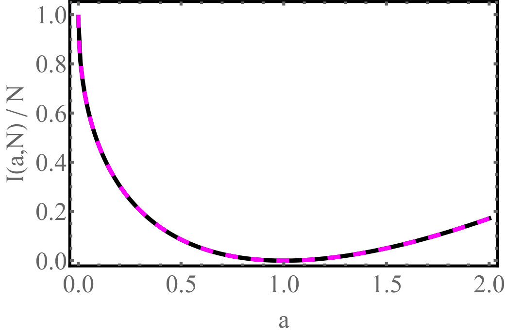 Figure 1
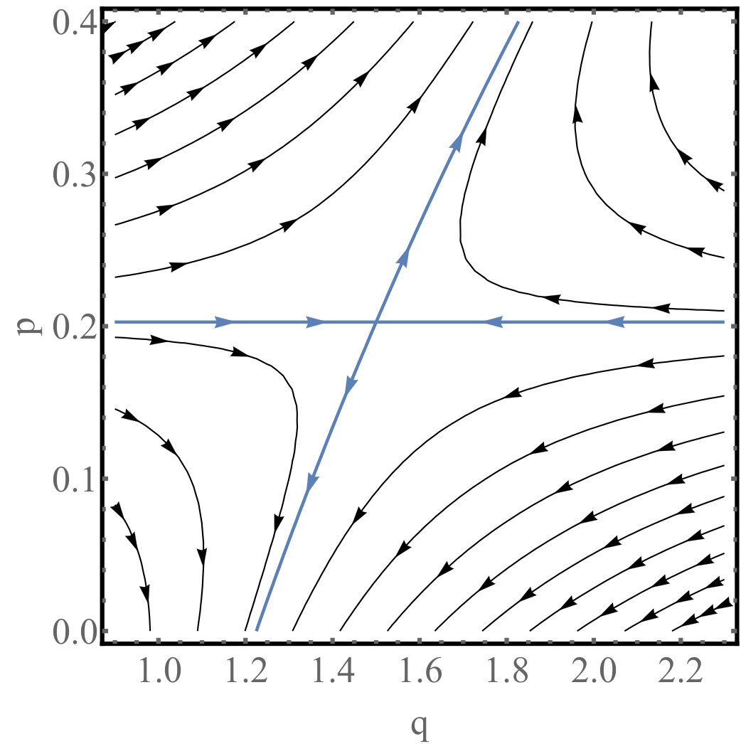 Figure 2
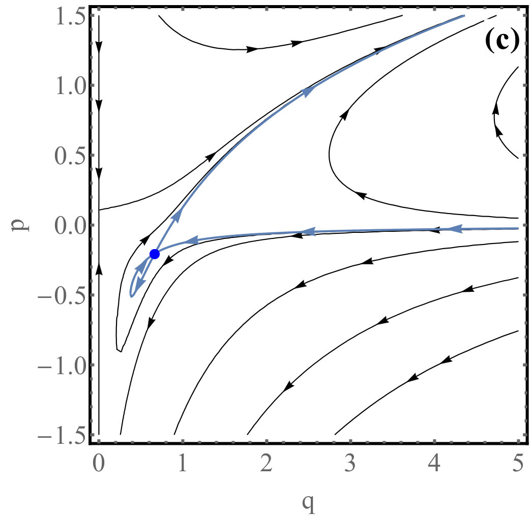 Figure 3
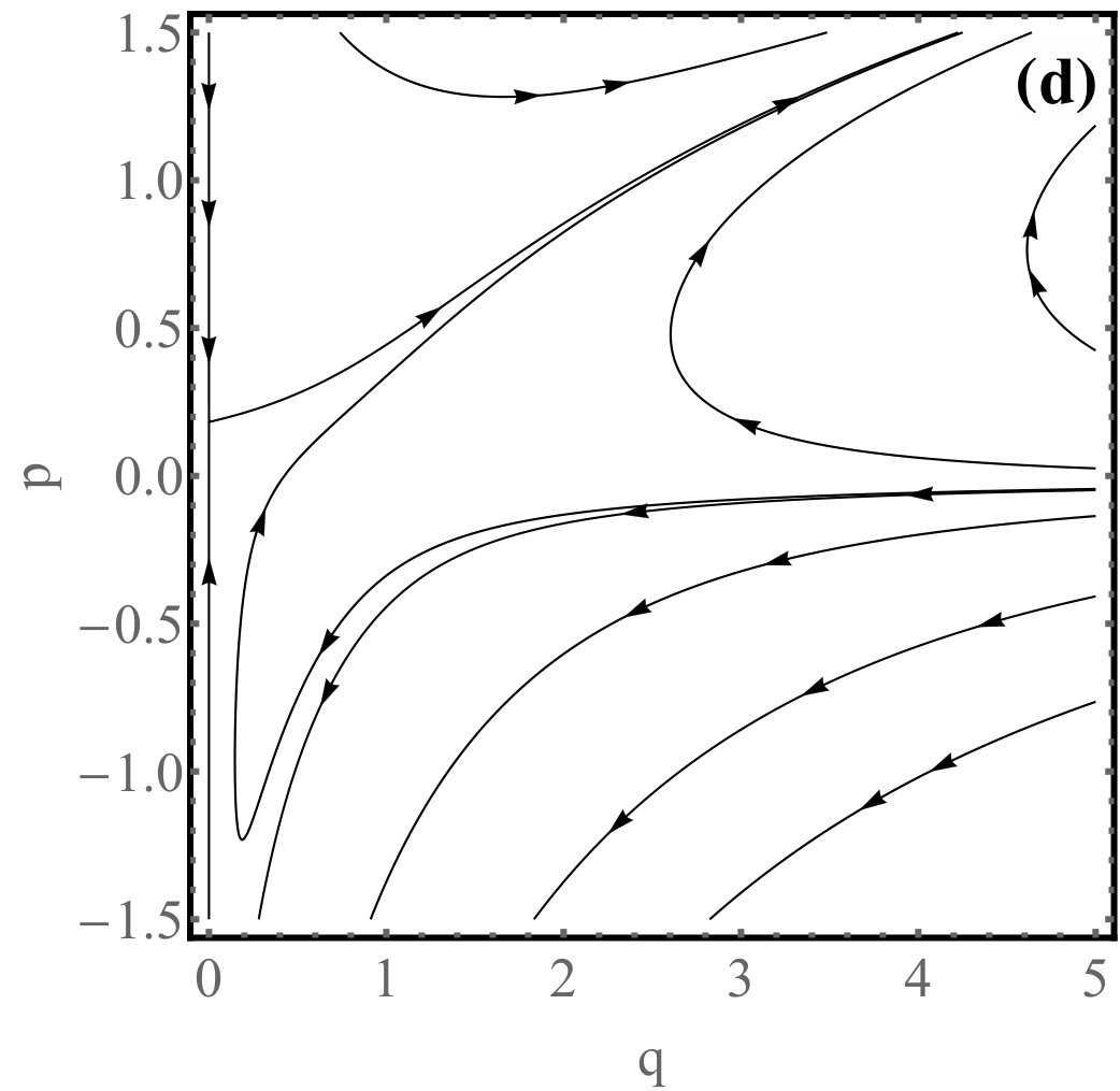 Figure 4
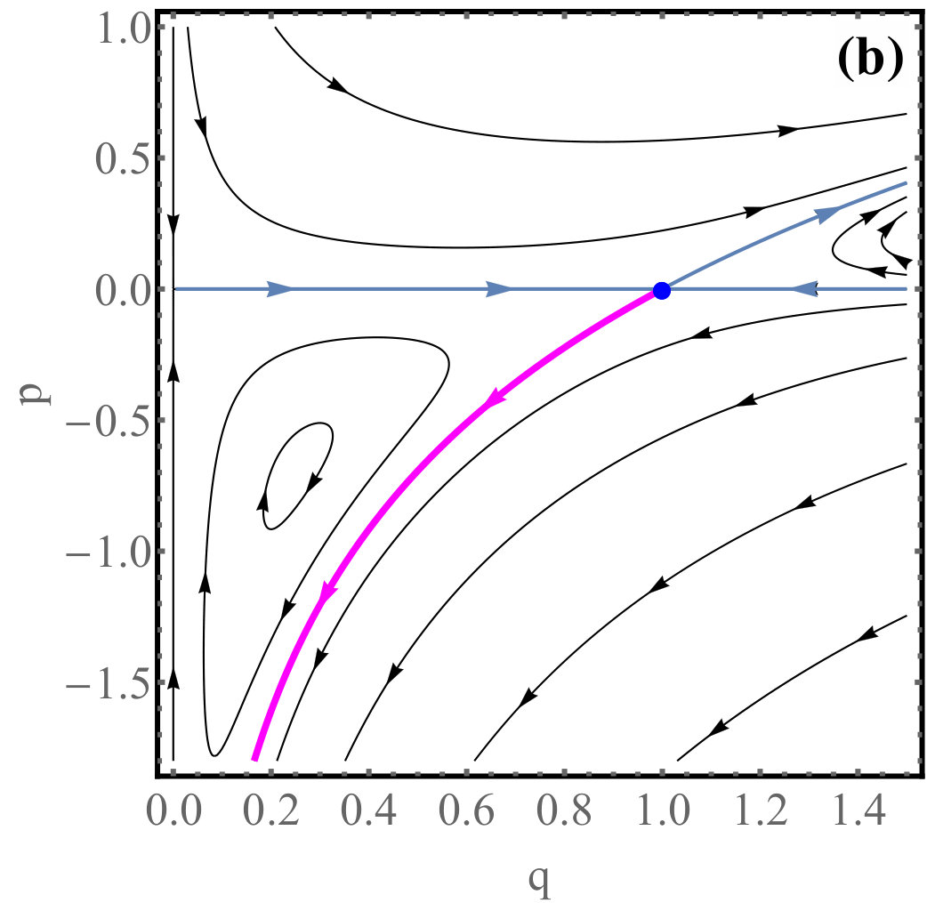 Figure 5
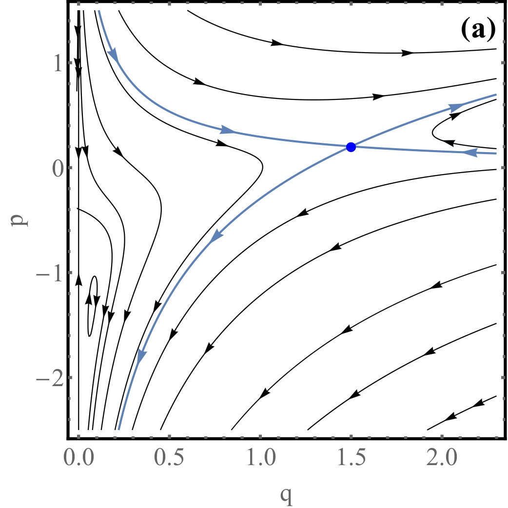 Figure 6
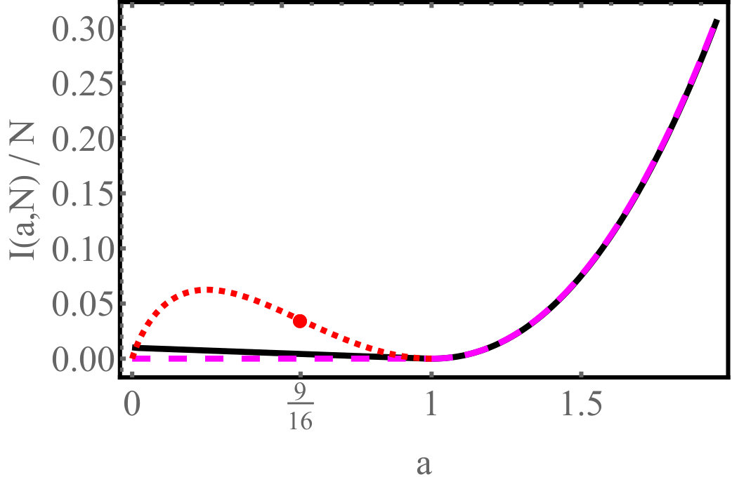 Figure 7
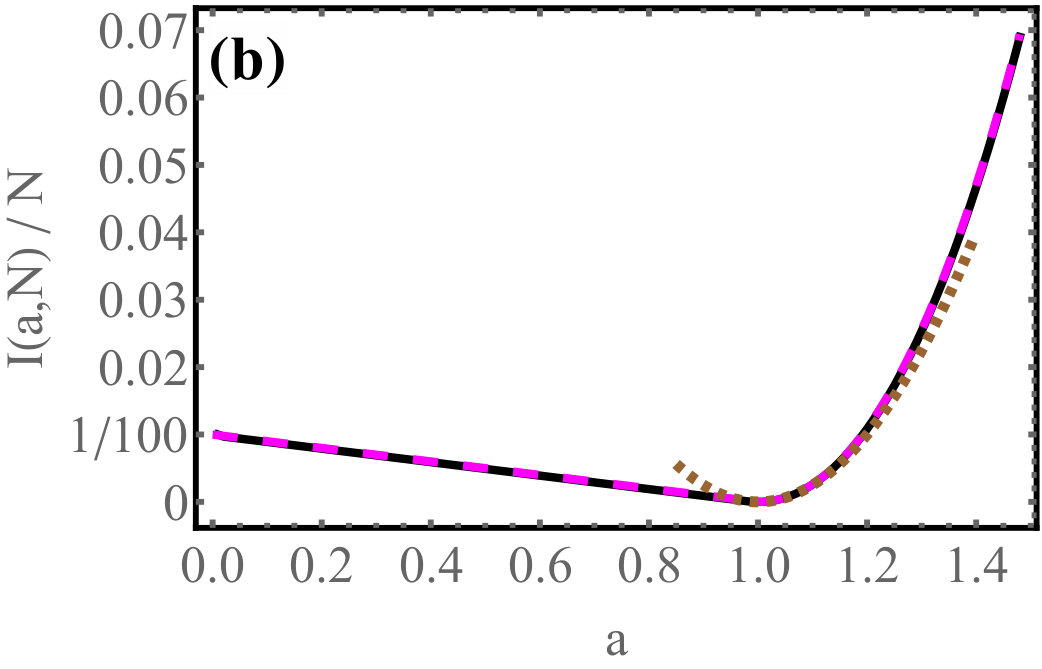 Figure 8
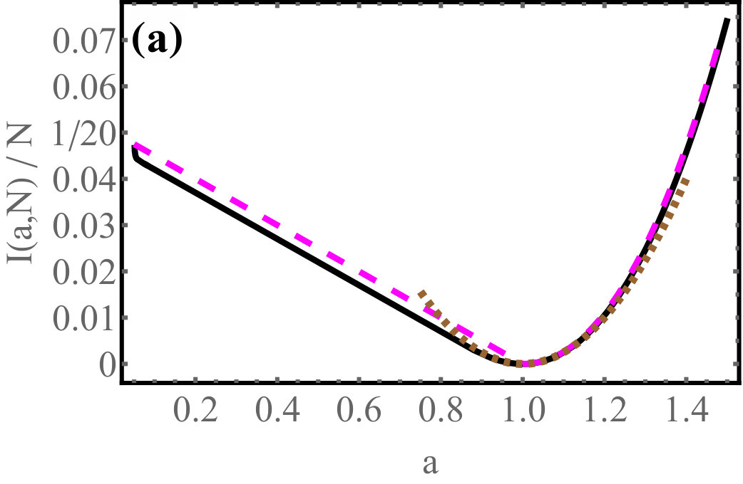 Figure 9
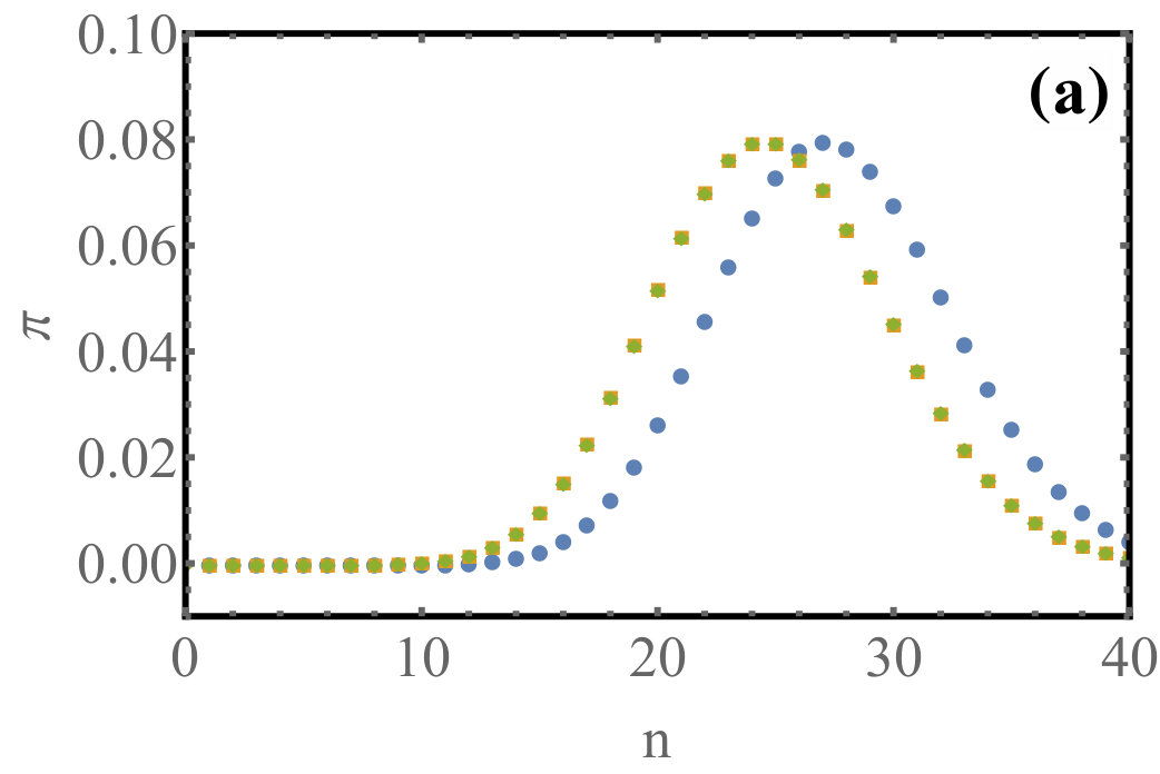 Figure 10
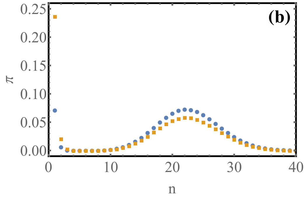 Figure 11
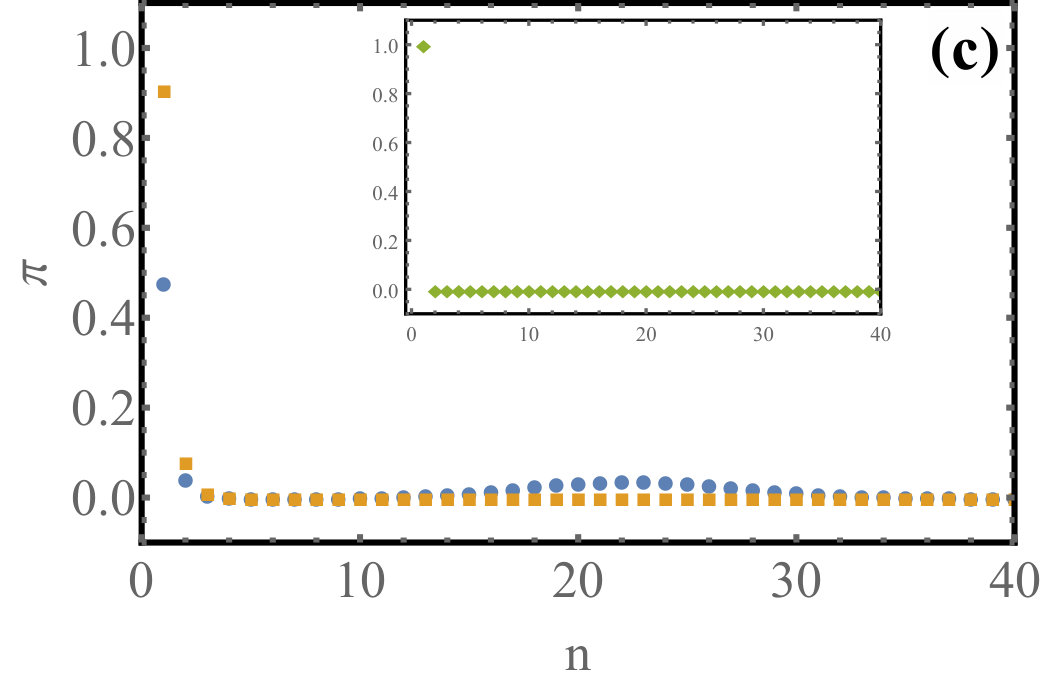 Figure 12
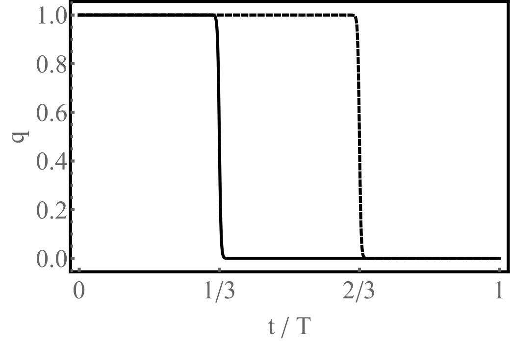 Figure 13
Peer Reviews
No public reviews on file for this paper yet. If you reviewed it on a platform where reviews are public (OpenReview, ICLR, NeurIPS, ICML), you can paste yours below so the community can read it here.
Videos
No videos yet. Explain this paper in a talk, walkthrough, or lecture? Add one.
A giant disparity and a dynamical phase transition in large deviations of the time-averaged size of stochastic populations
Pini Zilber
Naftali R. Smith
Baruch Meerson
Racah Institute of Physics, Hebrew University of Jerusalem, Jerusalem 91904, Israel
Abstract
We study large deviations of the time-averaged size of stochastic populations described by a continuous-time Markov jump process. When the expected population size in the steady state is large, the large deviation function (LDF) of the time-averaged population size can be evaluated by using a WKB (after Wentzel, Kramers and Brillouin) method, applied directly to the master equation for the Markov process. For a class of models that we identify, the direct WKB method predicts a giant disparity between the probabilities of observing an unusually small and an unusually large values of the time-averaged population size. The disparity results from a qualitative change in the “optimal” trajectory of the underlying classical mechanics problem. The direct WKB method also predicts, in the limit of , a singularity of the LDF, which can be interpreted as a second-order dynamical phase transition. The transition is smoothed at finite , but the giant disparity remains. The smoothing effect is captured by the van-Kampen system size expansion of the exact master equation near the attracting fixed point of the underlying deterministic model. We describe the giant disparity at finite by developing a different variant of WKB method, which is applied in conjunction with the Donsker-Varadhan large-deviation formalism and involves subleading-order calculations in .
I Introduction
Stochastic population models describe a multitude of processes in nature and society Delbrueck ; Bartlett ; Karlin ; Bailey ; Nisbet ; Andersson ; Allen ; Tsimring ; Allen2015 . Examples include reactions among particles, dynamics of biological populations, spread of diseases, inventions, opinions and rumors, dynamics of financial markets, and many other processes. A convenient mathematical description of stochastic populations is provided by Markov jump processes Kampen ; Gardiner . An important class of these processes has a nontrivial steady state, where the gain and loss processes balance each other on average. A standard characterization of a fluctuating steady state is in terms of its steady-state probability distribution. For a single population in a steady state this distribution, , describes the probabilities to observe individuals, which we will call particles.
In recent years there has been a growing interest in a different characterization of fluctuating steady states: by the probability distributions of long-time averages of observables, see Refs. Touchette2009 ; Touchette2018 and references therein. In the context of stochastic populations a natural quantity of this type is the long-time average of the (fluctuating) population size. For many stochastic systems, the probability of observing any value of the time-averaged size, which is different from the expected one, becomes exponentially small as the averaging time increases.
A similar property, and the ensuing large deviation function (LDF) that encodes it, have received much recent attention from physicists in the context of continuous diffusion processes, described by Langevin equations Touchette2009 ; Touchette2018 ; TouchettePRL2018 ; Lecomte . Recently this characterization has been extended MeersonZilber to one of the best known jump processes in physics: the Ehrenfest Urn Model EUM . The basic version of the Ehrenfest Urn Model involves two urns with identical balls. The balls hop randomly, one ball at a time, from one urn to the other. For non-interacting balls the LDF of the long-time average of the number of balls in a given urn can be calculated exactly MeersonZilber by using the Donsker-Varadhan (DV) large-deviation formalism DonskerVaradhan , which we briefly review below. If the balls interact, the DV formalism can still be used numerically MeersonZilber , but it does not allow for analytical solution. However, when the total number of balls is very large, one can circumvent the DV method and employ instead a WKB approximation, directly applied to the master equation Kubo ; Gang ; Dykman ; AssafMeerson . In this way one obtains a controlled large- approximation of the LDF MeersonZilber .
Here we follow this line of work and identify a class of stochastic populations, for which the direct WKB method predicts a giant disparity between the probabilities of observing an unusually small and an unusually large values of the time-averaged population size. This disparity results from a qualitative change of the character of the optimal (least-action) trajectory of an underlying Hamiltonian classical mechanics problem. The direct WKB method also predicts a jump in the second derivative of the LDF, which can be interpreted as a second-order dynamical phase transition. The sharp transition is smoothed by finite- effects, unaccounted for by the leading-order WKB approximation, but the giant disparity remains. We show it by developing a different version of WKB theory, which involves subleading-order WKB calculations and is used in conjunction with the DV large-deviation formalism.
Now let us be more specific. Consider a jump process which admits a nontrivial steady state, and denote the population size (the number of particles) in a specific realization of the process at time by . We are interested in the probability, , that the time averaged population size , defined as
[TABLE]
is equal to , where is the expected population size, and is a real non-negative number. When is very large, satisfies the large deviations principle, which states that any deviation from the expected value is exponentially unlikely to occur:
[TABLE]
The rate function is the focus of our interest. It is a non-negative function of that vanishes at its most probable value which, for , is . In the limit , is independent of the initial condition. An analytical calculation of is in general impossible. When , one can employ a direct WKB approximation Kubo ; Gang ; Dykman ; AssafMeerson , as it has been recently done for the Ehrenfest Urn Model MeersonZilber . In this approximation the - and -dependences of the rate function factorize MeersonZilber . In the class of models that we will work with here, the rate function , as predicted by the direct WKB approximation, is proportional to :
[TABLE]
It is natural to call the function the intensive rate function.
For many stochastic populations the intensive rate function is an analytic function of , and the Ehrenfest Urn Model provides one such example MeersonZilber . As we will see shortly, another such example is provided by the immigration-death process , a simple and well studied reversible jump process. However, as we find here, there is a class of population models where , as described by the direct WKB method, vanishes on the whole interval . This corresponds to a giant disparity between the probabilities of observing an unusually small and unusually large values of . Furthermore, the predicted is non-analytic at . We will identify this class of models and exemplify it by still another simple reversible process: the branching-coalescence process . Then we will obtain more accurate results for this model, by going beyond the direct WKB method.
Here is a plan of the remainder of the paper. In Sec. II we outline the direct WKB method and consider two simple examples: the immigration-death process and the branching-coalescence process. We show that the intensive rate function is analytic in the former case, and non-analytic and vanishing at in the latter. In Sec. III we apply WKB approximation, in the leading and subleading orders with respect to , to the DV method. In the leading order this calculation reproduces the results of the direct WKB method. In the subleading order the degeneracy is removed due to finite- effects. We also compute the probability distribution of the population size, conditional on a specified value of . We show that, in the phase-transition region of , the distribution is bimodal, which reflects the character of the optimal trajectories of the system in this region. We discuss our results and some possible generalizations in Sec. IV.
II Direct WKB method
II.1 General
We start this section by considering a general single-step jump process for a single population. A generalization to multiple-step processes is immediate Dykman ; EscuderoK ; AM2010 . The process is governed by the master equation Kampen ; Gardiner
[TABLE]
for the evolution of the probability of observing particles at time . The first two terms on the right describe the incoming rates into state from the states and , whereas the last term describes the total outgoing rate from state . We assume throughout this work that the birth and death rates and are such that Eq. (II.1) admits a nontrivial steady-state solution. We will also assume that the birth and death rates are disparate so that the expected population size in the steady state is large, and exploit the large parameter . Let us expand the process rates in the powers of . Introducing the rescaled population size , we obtain EscuderoK ; AM2010
[TABLE]
where and are assumed to be .
If one multiplies the master equation (II.1) by , sums it up over all possible values of and ignores fluctuations Kampen ; Gardiner , one arrives at the deterministic rate equation
[TABLE]
The stationary population, residing in a vicinity of , corresponds to an attracting fixed point of Eq. (6) at , so that and , where prime denotes the -derivative.
The direct WKB method for an analysis of fluctuations Kubo ; Gang ; Dykman ; AssafMeerson exploits the large parameter by applying the WKB ansatz
[TABLE]
directly to the master equation. Additionally, we assume , treat as a continuous variable, and evaluate the action at by Taylor expanding it around Kubo ; Gang ; Dykman :
[TABLE]
Using this expansion of in the WKB ansatz (7) and plugging the ansatz into the master equation (II.1), we arrive at an equation which involves , and in different orders of , and treat it order by order. In the leading order this procedure yields a Hamilton-Jacobi equation for the “action” Kubo ; Gang ; Dykman :
[TABLE]
where
[TABLE]
is the model-specific Hamiltonian. As one can see, the population size plays the role of the coordinate of an effective “particle”, whereas is the momentum. The action along a trajectory is given by
[TABLE]
where is the (conserved) energy of the “particle”. The constraint () can be accounted for by adding a term , where is a Lagrange multiplier, to the action. In the Lagrangian formulation the constrained Lagrangian is
[TABLE]
where is the unconstrained Lagrangian, corresponding to the unconstrained Hamiltonian . The constrained Hamiltonian is equal to LLMechanics
[TABLE]
where should be expressed through and from the relation . As a result, the constrained Hamiltonian takes the form MeersonZilber
[TABLE]
As one can see, the constraint is enforced via a simple additive term in the Hamiltonian. This simplicity occurs because does not depend on , see Eq. (12). The phase-space trajectories and satisfy the Hamilton’s equations
[TABLE]
Among all such trajectories, we must choose the one which satisfies appropriate boundary conditions and the condition
[TABLE]
which ultimately sets the value of . If there is more than one such trajectory, we must choose the “optimal” one which minimizes the action (11). Having found it, we can evaluate , where is its corresponding action.
In the Hamiltonian description the attracting fixed point of the deterministic rate equation (6) becomes a saddle point of the unconstrained Hamiltonian . For the constrained Hamiltonian (14) this saddle point is shifted. For finite the action depends on the initial condition , and must be minimized with respect to the final condition . As increases, the effective “particle” spends more and more time in a close vicinity of the above-mentioned shifted saddle point of the constrained Hamiltonian MeersonZilber . For this saddle point dominates both the action (11) (where the first term vanishes) and the integral over time in Eq. (17). Then, in view of the Eq. (17), the -value of this fixed point must be equal to . The corresponding value of can be obtained from the algebraic equation
[TABLE]
which follows from Eq. (15). At this stage we are already constraining the process by , so the Lagrange multiplier becomes unnecessary. The optimal action, evaluated at the saddle point, is very simple:
[TABLE]
Finally, combining Eqs. (2), (7) and (19), we obtain the intensive rate function , defined by Eq. (3):
[TABLE]
Equation (20) has quite a general form, and it also holds for multi-step processes. Let us specialize Eq. (20) to the single-step process (II.1). Using Eqs. (10) and (18), we obtain the value of at the fixed point:
[TABLE]
As a result, Eq. (20) yields
[TABLE]
so one only needs to know the leading-order terms of the birth and death rates (5). Equation (22) reproduces the recent result MeersonZilber for the rate function of the time-averaged number of balls in one of the urns in the Ehrenfest Urn Model.
II.2
As another simple example, consider the immigration-death process
[TABLE]
with the per-capita immigration rate and the per-capita death rate . The process rates are and . This simple process obeys the detailed balance condition
[TABLE]
where the equilibrium distribution is Poisson:
[TABLE]
Now we assume and and turn to the WKB description. We immediately note that the leading-order rates and are exact here. Figure 1 shows the phase portrait of the constrained Hamiltonian,
[TABLE]
The shifted saddle point is at . It exists for , and its coordinate can take any value from zero to infinity.
Plugging the rates and into Eq. (22), we obtain the intensive rate function of the long-time average population size in this system:
[TABLE]
The function is strictly convex. It vanishes at the expected value and is positive for all other . It is shown in Fig. 2 alongside with numerical results, obtained by the DV method DonskerVaradhan , which we briefly discuss in the beginning of Sec. III. The perfect agreement, even for a moderate value of , is explained by the fact that, for this simple process, the WKB result (27) is exact. The WKB result is also exact for the Ehrenfest Urn Model with non-interacting balls MeersonZilber .
II.3 : Giant disparity of probability and dynamical phase transition at
Expressions (20) and, for single-step processes, (22) are not always correct. Indeed, the shifted saddle point with coordinate may not exist, or it may be unaccessible for some initial conditions. But even if it exists and is accessible, there can be a different trajectory with a lesser action, which does not stay in a close vicinity of the shifted saddle point. We will illustrate these general arguments on the example of a well-known branching-coalescence process
[TABLE]
with per-capita rates and , respectively. This process exhibits nontrivial dynamics only if it starts from a nonzero number of particles, and we will suppose that this is the case. The branching rate is given by the product of the per-capita branching rate and the current population size . The coalescence rate is given by the product of the per-capita coalescence rate and the number of pairs in the population of particles, . As a result,
[TABLE]
This process also obeys the detailed balance condition (24), and the equilibrium distribution is again Poisson:
[TABLE]
However, as we will see now, the large deviation function of the long-time average population size is more interesting here than for the immigration-death process. Applying the direct WKB method and using Eqs. (5) and (29), we identify the leading-order rates and . Recklessly using Eq. (22), we would obtain the intensive rate function
[TABLE]
shown in Fig. 3 by the dotted line. This function is obviously non-convex for . Actually, it is non-convex, according to the supporting line definition of convexity, for all . This arises suspicion, and indeed Eq. (31) turns out to be incorrect on the whole interval .
In order to see why, let us explore the phase portrait of the system. The deterministic equation (6) takes the form . The attracting fixed point is again , but now there is also a repelling fixed point at . This fact turns out to be crucial, as the effective mechanical system can now stay for a long time at the fixed point without the need to “spend” any action. Let us see how it works. The phase portraits of the unconstrained Hamiltonian,
[TABLE]
is shown in Fig. 4b. The repelling and attracting fixed points of the deterministic dynamics become saddle points and , respectively. In addition, an elliptic fixed point appears at .
For the flow described by the constrained Hamiltonian,
[TABLE]
the three fixed points become -dependent. The saddle point of the unconstrained Hamiltonian becomes . It exists for . The nontrivial saddle point exists for , and the elliptic point exists for . At the latter two fixed points merge, and for they disappear: compare panels c and d in Fig. 4. As one can check, for all , the value of of the nontrivial saddle point is greater than or equal to ; the equality occurs at . The absence of a nontrivial saddle point with (see Fig. 4d) explains why Eq. (31) cannot be correct for .
What happens for ? Here the nontrivial saddle point is accessible for some initial conditions, and inaccessible for others. More importantly, there is a trajectory of a different type, which corresponds to , provides any specified value of and has a lesser action. This trajectory is closely related to the exact one-parameter family of instanton solutions of the unconstrained Hamilton equations:
[TABLE]
These solutions, depicted in Fig. 5, satisfy the boundary conditions , , and . They correspond to the zero-energy phase trajectory , indicated by the thick line on Fig. 4b. When , they can serve as approximate solutions on the finite interval , and they are accurate up to corrections which are exponentially small with respect to . Furthermore, one can always choose the constant so that condition (17) is satisfied for any . The action (11) for each of these trajectories is equal (again, up to exponentially small corrections in ) to
[TABLE]
Crucially, this action is independent of . As a result, the intensive rate function vanishes at and , and we arrive at
[TABLE]
Therefore, the probabilities of observing and are dramatically different. Notably, is continuous with its first derivative at . The second derivative, however, has a jump at which can be interpreted as a dynamical phase transition of second order. The appearance of a giant disparity in , and of a second-order phase transition, in a simple reversible one-population model is quite remarkable.
The sharp transition, however, is observed only in the limit . A valuable insight into finite- effects can be achieved if we go beyond the WKB method and try to interpret the unexpected result at in the language of the exact microscopic process . We can easily do it for one particular value of : . What is the probability to observe, for very large , the average population size equal to fn_nmin ? The only stochastic trajectory that can contribute to this average population size is the one where , while the branching process is suppressed for the whole time . The probability of the stochastic trajectory during the time is , hence . Consequently, in the limit , we get . On the other hand, vanishes at (for ), so that . As we expect the rate function to be convex, it must satisfy , in agreement with the first line of Eq. (36), predicted by the direct WKB method.
The direct-WKB prediction (36) for is presented in Fig. 3 alongside with numerical results obtained by the DV method DonskerVaradhan for . One can see excellent agreement for (which is not surprising, as in this regime the solution comes from the shifted saddle point). The numerical result at perfectly agrees with the exact result , quoted above. It follows immediately from , and the expected convexity of that
[TABLE]
The numerics indeed indicate a linear behavior of as a function of , with slope , so that the upper bound (37) is in fact very close to the actual value of . Our next goal will be to derive a subleading WKB asymptotic which describes the finite effects observed in the numerics.
III WKB for DV
III.1 DV method
The exact DV method DonskerVaradhan reduces the determination of the rate function in the limit to the solution of an eigenvalue problem. In most cases this eigenvalue problem can only be solved numerically. Figures 2 and 3 show such numerical solutions which we obtained for the processes and , respectively. In this section we will show how to solve this eigenvalue problem analytically, albeit approximately, by exploiting the large parameter . We will do it by developing a different version of WKB theory, which is applied to the DV eigenvalue problem.
We will start with a brief description of the DV method. Consider a general jump process, governed by a master equation of the form
[TABLE]
For a single-step process (II.1) is a tridiagonal matrix. The Gärtner-Ellis GartnerEllis theorem states that the rate function is given by the Legendre-Fenchel transform,
[TABLE]
of the scaled cumulant generating function , defined as
[TABLE]
where denotes averaging over possible values of . According to DV, is equal to the largest eigenvalue of an auxiliary operator :
[TABLE]
where
[TABLE]
is a tilted version of the operator , which is the Hermitian conjugate of . For any value of , the Legendre-Fenchel transform (39) associates a value of . We will denote it by , so that
[TABLE]
We used (a truncated version of) this method to perform our numerical calculations.
III.2 expansion and WKB for DV
Employing the small parameter , we can seek the rate function perturbatively:
[TABLE]
In the absence of the phase transition in the limit of , both and are of order . For the branching-coalescence process (and other models which exhibits a phase transition of this type) and are of order only for . For we should expect , so the rate function is
[TABLE]
It is this, more interesting case, that we will focus on lessinteresting . We additionally assume that , as the WKB approximation does not hold for . As we will see, the WKB approximation also breaks down for very close to , and we will use a different approximation there.
By virtue of Eqs. (43) and (45), must be of order , and must be of order , so we should set
[TABLE]
where the unknown functions and are of order 1. The last equality in Eq. (47), where we introduce a new function , follows from the demand that does not depend on . Plugging Eqs. (46) and (47) into Eq. (39) yields
[TABLE]
Let us determine the function , specializing our calculations to the branching-coalescence model. The auxiliary operator of the DV method is
[TABLE]
where we have set , see Eq. (46). Let us consider the eigenvalue problem for the right eigenvector ,
[TABLE]
and find the maximal eigenvalue by using WKB approximation. As in the direct WKB method, we define , make a WKB ansatz
[TABLE]
and treat as a continuous variable, so that
[TABLE]
When we plug this ansatz into Eq. (50), the factor will cancel out, so we will ignore it from now on. Before making the ansatz, we expand in the powers of :
[TABLE]
so that
[TABLE]
Now we make the ansatz and obtain
[TABLE]
In the order we obtain a time-independent Hamilton-Jacobi equation
[TABLE]
with the Hamiltonian , defined in Eq. (32). The quantity plays the role of the (conserved) energy. We immediately notice that , and therefore , do not depend on , so that we can evaluate them at . But for , the right eigenvector, which corresponds to the maximal eigenvalue, is a constant which can be set to be Touchette2018 . As a result, , and Eq. (56) yields . This result coincides with the one obtained by the direct WKB method, where we found that the energy of the optimal trajectory is zero for any fn_eigenvector .
The sub-leading correction emerges from the terms of Eq. (III.2). Using the equalities , we obtain
[TABLE]
This is again a time-independent Hamilton-Jacobi equation, with the Hamiltonian . Solving Eq. (57) for , we see that diverges at unless we set . As a result, fn_subleading . The divergence of at is not dangerous, because at , that is at , our continuous WKB approximation for breaks down anyway.
By virtue of and Eqs. (41) and (47), we obtain
[TABLE]
Before we use this result in Eq. (48), we will show that is bounded from below by . Let us return to the exact eigenvalue problem (50):
[TABLE]
In particular, for we obtain
[TABLE]
All components of the eigenvector, corresponding to the maximum eigenvalue, and in particular and , must have the same sign Touchette2015 ; Touchette2018 . (A familiar analog is a ground-state wave function which does not have nodes.) Therefore, the right hand side of Eq. (60) must be positive. Using the scalings and [see Eqs. (41), (46) and (47)], we obtain
[TABLE]
To avoid excess of accuracy, we ignore the term and obtain the inequality . Applying now the WKB result (58), we see that . To remind the reader, this result is valid only in the WKB regime. Using this bound and Eq. (58) in Eq. (48), we obtain
[TABLE]
that is the maximum is reached at the boundary. The nonzero rate function (62) removes the degeneracy at , that we previously observed at .
The continuous WKB theory breaks down at , so Eq. (62) is inapplicable there. It is also inapplicable too close to , where the WKB action is small. Fortunately, in a close vicinity of one can approximate AssafMeerson ; MeersonZilber the exact master equation of the jump process by a continuous Fokker-Planck equation, using the Van Kampen system-size expansion Kampen . This leads to an effective Ornstein-Uhlenbeck process, and we obtain (see e.g. Eq. (49) in Ref. Touchette2018 )
[TABLE]
corresponding to the Gaussian asymptotic of as a function of near the expected value . Equation (63) also follows from a Taylor expansion around of the branch of from Eq. (36). Notably, the smooth Gaussian asymptotic clearly implies that the second-order phase transition is an attribute of the leading-order WKB approximation. Using Eqs. (62) and (63), we can establish the applicability condition of Eq. (62) at close to : . Putting everything together, we obtain
[TABLE]
The asymptotics (66) and (67) coincide in their joint region .
Our numerics, see Fig. 6, show that the exact rate function is strictly convex. This feature is most clearly observed at not too large or at small . The approximate expression (64) is not strictly convex, but it is natural to assume that strict convexity will appear in the next order of the perturbation procedure minus_infinity . Figure 6 compares the asymptotics (64)-(67) with numerical results, obtained by the DV method DonskerVaradhan , for and . As one can see, the WKB approximation improves for larger .
Figure 7 shows our numerical results for the stationary distribution of the branching-annihilation process, conditioned on a given value of (or ). This distribution is given by the properly normalized product of the right and left eigenvectors, for a fixed value of (or ) Chetrite2013 ; Touchette2015 . Remarkably (but a posteriori not surprisingly), for the conditional distribution is bimodal: one of its two peaks is at , the other is at . As increases, the two peaks become well separated, and the area under the peak at approaches , whereas the area under the peak at approaches . This is in a remarkable agreement with the prediction of our direct WKB analysis of Sec. II.3. Indeed, for the optimal trajectory is such that the population has size for time and then, after a short transient, size (which, in the direct WKB method, is indistinguishable from zero) for time .
IV Discussion
Time-averaged quantities provide a useful characterization of stochastic populations. Here, using a WKB approximation, we observed, at , a dynamical phase transition and a giant disparity in the large deviation function (LDF) of the time-averaged population size of the branching-coalescence process. These effects result from a qualitative change in the “optimal” trajectory of the underlying Hamiltonian classical mechanics problem. The phase transition is in fact smoothed at finite , but the probabilities of observing unusually small and unusually large values of the time-averaged population size remain dramatically different. In order to resolve the degeneracy at , obtained in the leading WKB order, we developed a different version of WKB method, which is applied in conjunction with the Donsker-Varadhan large-deviation formalism and goes beyond the leading-order calculations in . A similar in spirit methodology has been recently implemented for a continuous diffusion process Derrida , where a (very different) singularity of a large deviation function, and its regularization, have been studied.
From a more general perspective, our work provides an additional example of a singularity in a LDF of a time-integrated fluctuating quantity which appears in the weak-noise limit . A somewhat similar in spirit singularity (also of second order) appears in the LDF of the time- and space-integrated current in certain diffusive lattice gases in systems with periodic boundaries Bertini2006 ; Bodineau2007 . The details, however, are quite different.
Our results, obtained for the branching-annihilation model, can be immediately generalized to a whole family of single-species stochastic population models, which have a nontrivial (that is, non-empty) steady state, corresponding to a non-trivial attracting fixed point of deterministic theory. A sufficient condition for the emergence of a giant probability disparity at large , and a second-order dynamical phase transition in the limit of , is the presence of a repelling fixed point at . We can even relax the demand of the non-empty steady state by conditioning the process on the population survival by the time over which the long-time average is calculated.
It would be interesting to complete our calculations of in the regions and , where WKB theory breaks down. It would be also interesting to study statistics of the time-averaged population size for stochastic populations which exhibit switches between two metastable states. In the deterministic description, these populations have two attracting fixed points, and a repelling point in between. A host of additional interesting questions concerns multi-population systems which describe coexistence of species.
Finally, a giant disparity and a second-order dynamical phase transition should also appear, in the weak-noise limit, in LDFs of time-averaged quantities in continuous systems with multiplicative noise. In analogy to our work, this can happen in the presence of an attracting fixed point and a repelling fixed point in the deterministic limit.
ACKNOWLEDGMENTS
We are grateful to Hugo Touchette and Tal Agranov for useful discussions, and acknowledge support from the Israel Science Foundation (Grant No. 807/16). N.R.S. was supported by the Clore Foundation.
The reference list from the paper itself. Each links out to its DOI / PubMed record.
- 1(1) M. Delbrück, J. Chem. Phys. 8 , 120 (1940).
- 2(2) M. S. Bartlett, Stochastic Population Models in Ecology and Epidemiology (Willey, New York, 1960).
- 3(3) S. Karlin and J. Mc Gregor, Stochastic Models in Medicine and Biology (University of Wisconsin Press, Madison, 1964).
- 4(4) N. T. J. Bailey, The Mathematical Theory of Infectious Diseases and its Applications (Griffin, London, 1975).
- 5(5) R. M. Nisbet and W. S. C. Gurney, Modelling Fluctuating Populations (Wiley, New York, 1982).
- 6(6) H. Andersson and T. Britton, Stochastic Epidemic Models and their Statistical Analysis (Springer, New York, 2000).
- 7(7) L. Allen, An Introduction to Stochastic Processes with Applications to Biology (Pearson Education, Upper Saddle River, NJ USA, 2003).
- 8(8) L.S. Tsimring, Rep. Prog. Phys. 77 , 026601 (2014).