Cutoff on Ramanujan complexes and classical groups
Michael Chapman, Ori Parzanchevski

TL;DR
This paper proves the total-variation cutoff phenomenon for simple random walks on Ramanujan complexes of type A_d, providing explicit generators for classical groups where cutoff occurs, advancing understanding of mixing times on expanders.
Contribution
It establishes total-variation cutoff for random walks on Ramanujan complexes and identifies explicit generators for classical groups with this property.
Findings
Proves cutoff for Ramanujan complexes of type A_d.
Provides explicit generators for PGL_n(\u021b_q) with cutoff.
Advances understanding of mixing times on sparse expanders.
Abstract
The total-variation cutoff phenomenon has been conjectured to hold for simple random walk on all transitive expanders. However, very little is actually known regarding this conjecture, and cutoff on sparse graphs in general. In this paper we establish total-variation cutoff for simple random walk on Ramanujan complexes of type . As a result, we obtain explicit generators for the finite classical groups for which the associated Cayley graphs exhibit total-variation cutoff.
Click any figure to enlarge with its caption.
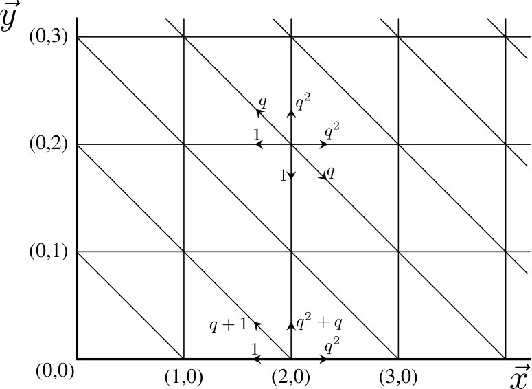 Figure 1
| 2 | ||
| 3 | ||
| 4 | ||
| 5 | ||
| 6 | ||
| 7 |
Peer Reviews
No public reviews on file for this paper yet. If you reviewed it on a platform where reviews are public (OpenReview, ICLR, NeurIPS, ICML), you can paste yours below so the community can read it here.
Videos
No videos yet. Explain this paper in a talk, walkthrough, or lecture? Add one.
Cutoff on Ramanujan complexes
and classical groups
Michael Chapman
and
Ori Parzanchevski
Abstract.
The total-variation cutoff phenomenon has been conjectured to hold for simple random walk on all transitive expanders. However, very little is actually known regarding this conjecture, and cutoff on sparse graphs in general. In this paper we establish total-variation cutoff for simple random walk on Ramanujan complexes of type (). As a result, we obtain explicit generators for the finite classical groups for which the associated Cayley graphs exhibit total-variation cutoff.
1. Introduction
The -mixing time of a finite Markov chain is the earliest time at which the distribution on states becomes -close to the stationery one, regardless of the starting distribution. There are several distance functions which one may use, and we focus on , or total-variation (see (1.1)). The parameter can be thought of as a measure of “standards”: for example, in a professional poker tournament one expects the dealer to shuffle the decks longer than in an amateur one. Loosely speaking, a sequence of Markov chains is said to exhibit the cutoff phenomenon if it is insensitive to ones’ standards. Namely, whether one seeks to be at most away from the stationary distribution or at most away from it, it will roughly take the same amount of time. In other words, for a long period of time the distribution is at almost maximal distance from stationery, and then over a short period of time it mixes almost completely. This counter-intuitive phenomenon was first demonstrated by Diaconis–Shahshahani and Aldous [diaconis1981generating, aldous1983random], and was subsequently shown to hold in many naturally occurring Markov chains (see the surveys [Diaconis1996cutoffphenomenonfinite, SaloffCoste2004RandomWalksFinite]). Common to all of these examples is that the number of legal moves grows together with the number of states.
The case of a bounded number of legal moves – for example, simple random walk (SRW) on a family of graphs with bounded degrees – turned out to be more resistant, and much less is known about it. In 2004, Peres has conjectured that SRW on every family of transitive bounded degree expanders exhibits the cutoff phenomenon [AmirDembo2004SharpThresholdsMixing], even though at the time *no family of bounded degree expanders was known to do so. In [Lubetzky2010Cutoffphenomenarandom], Lubetzky and Sly used probabilistic methods to show that random regular graphs exhibit cutoff a.a.s.; The next big breakthrough was achieved by Lubetzky and Peres [lubetzky2016cutoff], who showed that SRW on all Ramanujan graphs (which are optimal expanders) exhibit cutoff. A main ingredient of [lubetzky2016cutoff] is to show first that non-backtracking random walk (NBRW) on Ramanujan graphs exhibits cutoff at an optimal time. The last assertion was generalized in [Lubetzky2017RandomWalks] to the context of Ramanujan complexes, which are high-dimensional analogues of Ramanujan graphs, defined in [li2004ramanujan, Lubotzky2005a]. In the paper [Lubetzky2017RandomWalks], Lubetzky, Lubotzky and the second author establish optimal-time cutoff for a large family of asymmetric random walks on the cells of these complexes (in the graph case, NBRW is an asymmetric walk on edges). However, the techniques of [Lubetzky2017RandomWalks] cannot be applied neither to any symmetric *random walk, nor to any walk on vertices.
The goal of the current paper is to establish cutoff for SRW on Ramanujan complexes arising from the group over a non-archimedean local field. Interestingly, while SRW on vertices only “sees” the -skeleton of the complex, our proof makes use of asymmetric random walks on cells of *all *dimensions of the complex, showing that the high-dimensional geometry can play an important role even when studying walks on graphs. A main motivation to study these complexes is the study of expansion in simple groups: the finite groups admit a Cayley structure of a Ramanujan graph due to Lubotzky, Phillips and Sarnak [LPS88], whereas the groups for general can be endowed with a Cayley structure which is the -skeleton of a Ramanujan complex. Thus, we establish here cutoff for SRW on the groups , with respect to the appropriate generators. We remark that the situation in the case is even more striking than in the graph case : by Kazhdan’s property , for every generating set of gives rise to an expander family of Cayley graphs of [Margulis1973ExplicitKazhdan], but except for the case which we handle in this paper, it is unknown whether these families exhibit cutoff or not.
We now move on to rigorous terms. Let be a connected directed graph (digraph), which we assume for simplicity to be -out and -in regular. Consider random walk on starting at a vertex with uniform transition probabilities, and denote by its distribution at time . The -mixing time of is
[TABLE]
where is the uniform distribution on (the vertices of ), and is the total-variation norm:
[TABLE]
A family of digraphs is said to exhibit cutoff if for every . The cutoff is said to occur at time , if for every there exists a window of size , such that for large enough. If we say that the cutoff is optimal, since a -regular walk cannot mix in less steps.
Recall that a connected -regular graph is called a Ramanujan graph if its adjacency spectrum is contained in .
Theorem** ([lubetzky2016cutoff]).**
The family of all -regular Ramanujan graphs exhibits (1) cutoff for SRW at time , with a window of size ; (2) optimal cutoff for NBRW (at time ), with a window of size .
In [lubetzky2016cutoff] SRW-cutoff is first reduced to optimal NBRW-cutoff, by studying the distance of SRW on the tree from its starting point. To obtain optimal cutoff for NBRW new spectral techniques are developed for analyzing non-normal operators.
To see how the notion of Ramanujan graphs generalizes to higher dimension, recall that is the -adjacency spectrum of the -regular tree, which is the universal cover of every -regular graph [Kesten1959]. In accordance, *Ramanujan complexes *are roughly defined as finite complexes which spectrally mimic their universal cover; for a precise definition see §2. In [Lubetzky2017RandomWalks], a vast generalization of part (2) of the theorem above is proved: say that a walk rule is collision-free if two walkers which depart from each other can never cross paths again.
Theorem** ([Lubetzky2017RandomWalks]).**
Let be an affine Bruhat-Tits building (see §2.1), and fix a collision-free walk rule on cells of . The family of Ramanujan complexes with universal cover exhibit optimal cutoff w.r.t. the corresponding walk rule on them.
This recovers NBRW on Ramanujan graphs, since NBRW is indeed collision-free on the edges of the tree. In higher dimension, NBRW is not collision-free anymore, but in [Lubetzky2017RandomWalks, §5.1] it is shown that collision-free walks do exist,* *on cells of every dimension, except for vertices. As SRW is not collision-free, the techniques of [Lubetzky2017RandomWalks] cannot address it (in fact, they cannot address any operator on vertices - see [Parzanchevski2018RamanujanGraphsDigraphs, Rem. 3.5(b)]).
The goal of this paper is to establish cutoff for SRW on Ramanujan complexes. We fix a non-archimedean local field with residue field of size , and denote by the Bruhat-Tits building associated with .
Theorem 1.1** (Main theorem).**
The family of all Ramanujan complexes with universal cover exhibits total-variation cutoff for SRW at time , with a window of size . The constant is determined in (4.2), and for each is a rational function in of magnitude (see Table 1).
We emphasize that the graphs underlying these walks are not Ramanujan graphs when . For example, in the two-dimensional case (where ), the -skeleton of is a -regular graph. If it was a Ramanujan graph, its second largest adjacency eigenvalue would be bounded by , but in truth this eigenvalue equals (cf. [saloff1997transition, li2004ramanujan]), reflecting the abundance of triangles in . In this case, the cutoff is achieved at time (see Theorem 3.1).
A motivation for our result which does not require the notions of Ramanujan complexes or buildings, is the study of expansion in finite simple groups (see [Breuillard2018Expansionsimplegroups] for a recent survey). A celebrated result of Lubotzky, Phillips and Sarnak [LPS88] uses the building of to show that the groups have explicit generators for which the resulting Cayley graphs are Ramanujan, so that [lubetzky2016cutoff] yields total-variation cutoff for SRW on these groups. Turning to , the work of [lubetzky2016cutoff] does not apply anymore, since it is not known whether have generators which yield Ramanujan Cayley graphs. Nevertheless, by considering the building of , it was shown by Lubotzky, Samuels and Vishne ([Lubotzky2005b], see also [sarveniazi2007explicit]) that the groups have explicit generators, for which the resulting Cayley graph is precisely the -skeleton of a Ramanujan complex of type . For , such generators can also be given using the building of [Evra2018RamanujancomplexesGolden, Ballantine2018ExplicitCayleyRamanujan]. We thus achieve:
Corollary 1.2**.**
- (1)
Fix and a prime power . The family has an explicit symmetric set of (Gaussian binomial coefficients) generators exhibiting TV-cutoff. 2. (2)
For and infinitely many pairs of primes , the family has an explicit symmetric set of generators exhibiting TV-cutoff (at time ).
We remark that even though this is a claim on Cayley graphs, the proof makes use of the high-dimensional geometry of their clique complexes!
Let us briefly explain our strategy for proving Theorem 1.1. Given a walk on , we lift it to a walk on , and then project it to a sector , which can be identified with the quotient of by the stabilizer of the starting point of the walk. If is a -regular graph then is the -regular tree, and is simply an infinite ray which we identify with : SRW on then projects to a -biased walk on this ray, and the projected location of the walker is precisely its distance from the starting point. On the other hand, this point is also the projection to of all terminal vertices of non-backtracking walks of length ; combining this with the optimal cutoff for NBRW is used to establish SRW cutoff in [lubetzky2016cutoff].
For the building of dimension , the so called *Cartan decomposition *gives an isomorphism , and the projected walk from on is an explicit, homogeneous, drifted walk on (with appropriate boundary conditions). Following the Lubetzky-Peres strategy, we would have liked to use this walk to reduce SRW-cutoff to some collision-free walk from [Lubetzky2017RandomWalks], for which optimal cutoff is already established. However, the terminal vertices of the various walks studied in [Lubetzky2017RandomWalks] are all located on the special rays in which correspond to the standard axes in . This is enough for the graph case (when ), but not in general. Our solution combines all the walks from [Lubetzky2017RandomWalks], using cells of all positive dimensions. For each point , we construct a concatenation of collision-free walks on cells of different dimensions, so that the possible paths of the walk terminate in a uniform vertex in the preimage of in . The results of [Lubetzky2017RandomWalks, Parzanchevski2018RamanujanGraphsDigraphs] are then used to bound the total-variation mixing of the corresponding concatenated walk on a Ramanujan complex.
For the convenience of the reader, we have divided the proof to the two-dimensional case (namely ) in §3, and the general case in §4. The case of is considerably simpler, due to the fact that it has additional symmetry: in this case acts transitively on the cells of every dimension of (see [kang2014zeta, Golubev2013triangle, Kaufman2019Freeflagsover] for detailed combinatorial studies of .) In addition, it is easier to visualize (see Figure 3.1), and some computations can be made more explicit and give sharper bounds.
Acknowledgement*.*
The authors are grateful to Ori Gurel-Gurevich for his help with proving Prop. 4.2. They also thank Eyal Lubetzky, Alex Lubotzky and Nati Linial for helpful discussions and encouragement. M.C. was supported by ERC grant 339096 of Nati Linial and by ERC, BSF and NSF grants of Alex Lubotzky. O.P. was supported by ISF grant 2990/21.
2. Preliminaries and notations
We briefly recall the notion of Bruhat-Tits buildings of type and the Ramanujan complexes associated with them. For a more detailed introduction, we refer the reader to [li2004ramanujan, Lubotzky2005a, Lubotzky2013].
2.1. Bruhat-Tits buildings
Let be a nonarchimedean local field with ring of integers , uniformizer , and residue field of size . The simplest examples are with , and with . Let and , which is a maximal compact subgroup of . The Bruhat-Tits building of type associated with is an infinite, contractible, -dimensional simplicial complex, on which acts faithfully. Denoting by the cells of of dimension , the action of on is transitive both on and . Furthermore, there is a vertex, which we denote by , whose stabilizer is , so that can be identified with left -cosets in . In this manner each vertex is associated with the -homothety class of the -lattice . A collection of vertices forms an -cell if, possibly after reordering, there exist scalars such that
[TABLE]
It follows that the link of a vertex in can be identified with the spherical building of , the finite complex whose cells corresponds to flags in . In particular, its vertices correspond to nonzero proper subspaces of , so that the degree of the vertices in is
[TABLE]
(see examples in Table 1). The vertices of are colored by the elements of , via
[TABLE]
and this coloring makes a -partite complex, namely, every -cell contains all colors. For , we say that an ordered cell is of *type one *if for , and we denote by all -cells of type one.
2.2. Ramanujan complexes
A *branching operator *on a set is a function By a *geometric *operator on we mean a branching operator on some subset of the cells of (e.g., all cells of dimension ), which commutes with the action of . If is a torsion-free lattice in then the quotient is a finite complex, equipped with a covering map , and induces a branching operator on the cells in , via . A function on is considered *trivial *if its lift to a function on is constant on every orbit of , and an eigenvalue of is called trivial if its eigenfunction is trivial. Denote by the space of trivial functions, and by its orthogonal complement.
Definition 2.1**.**
The complex is called a *Ramanujan complex *if for every geometric operator on , the nontrivial spectrum is contained in the spectrum of acting on .
In the above notations, we denote by the digraph with vertices , and edges , and similarly for the induced digraph on .
Theorem 2.2** ([Lubetzky2017RandomWalks, Thm. 3 and Prop. 5.3]).**
Let be a -regular geometric operator on . If is collision-free and is a Ramanujan complex, then is a -normal Ramanujan digraph (where
This requires some explanation. A -regular digraph is called:
- (1)
*collision-free *if it has at most one directed path between any two vertices; 2. (2)
-normal if its adjacency matrix is unitarily similar to a block diagonal matrix with blocks of size at most ; 3. (3)
a* Ramanujan digraph *if the spectrum of is contained in .
Denoting by the orthogonal complement to all -eigenfunctions with eigenvalue of absolute value , we have:
Theorem 2.3** ([Parzanchevski2018RamanujanGraphsDigraphs, Prop. 4.1]).**
If is a -regular -normal digraph with , then \left\|\vphantom{\big{|}}\smash{A_{\mathcal{D}}^{\ell}\big{|}_{L_{0}^{2}(\mathcal{D})}}\right\|_{2}\leq{\ell+r-1\choose r-1}k^{r-1}\lambda^{\ell-r+1}.
In particular, if is a -regular -normal Ramanujan digraph, then we have for every , so that
[TABLE]
2.3. Cartan decomposition
With the notations of §2.1, the fundamental apartment is the subcomplex of induced by all translations of by diagonal matrices in . Geometrically, is a simplicial tessellation of the affine space . The edges in are as follow: every vertex is connected to where runs over all non-constant binary vectors, i.e. (here and denote the all-zero and all-one vectors in , respectively).
We denote by the sector in induced by , where
[TABLE]
It is easy to see that is a fundamental domain for the action of (the so called spherical Weyl group) on . We identify with via
[TABLE]
thereby giving a graph structure. Denote by the boundary of , which corresponds to . Except at , the edges are the same as in , parameterized by . For , it might happen that , e.g. when , and one obtains the appropriate terminus of by reordering the entries of in descending order, and then dividing it by its last coordinate if it is not . The case of is depicted in Figure 3.1.
The Cartan decomposition for states that
[TABLE]
and the proof is a simple exercise (see e.g. [Goldfeld2011AutomorphicrepresentationsL, §13.2]). It follows that can also be identified with the quotient of by , and we denote the obtained projection from to by . In conclusion, we have identified four complexes: .
3. The case
In this section is the two-dimensional Bruhat-Tits building of . The -skeleton of is a -regular graph, with , where is the size of the residue field of .
Theorem 3.1**.**
Let be a Ramanujan complex with vertices. Then SRW on the underlying graph of has total-variation cutoff at time with a window of size .
3.1. A lower bound on the mixing time
Throughout this section we fix . Denote by the -ball around , i.e. the vertices of graph distance at most from in . First, we show that the ball of radius
[TABLE]
can cover only a small fraction of any -vertex quotient of :
Proposition 3.2**.**
For large enough, .
Proof.
Given , the -sphere is shown in [Evra2018RamanujancomplexesGolden] to be of size
[TABLE]
Thus, one can crudely bound the size of the -ball by , hence
[TABLE]
for large enough. ∎
Let be a SRW on starting at . We would like to determine until when does the walk remains in the -ball around with high probability. Since the distance from is -invariant, we have for , which leads us to consider the projection of by . In this manner, we obtain a (non-simple) random walk on , and we define
[TABLE]
Recall that we identified by mapping to , and the edges in (except at the boundary) are - see Figure 3.1.
Let and be the boundary lines of (the and axes in Figure 3.1). The transition probabilities of the projected random walk are as follows: from there is a probability of of moving to and to . Outside the boundary, the edge is taken with probability . On , the edges with are folded back in, giving the probabilities shown in Figure 3.1, and on the folding is symmetric.
Denote and , which measure the distance of the projected walk from the boundary. Clearly, . We consider , and as random walks on starting at zero.
Proposition 3.3**.**
The walks and are transient.
Proof.
We treat only , and the proof for is analogous. Although the distribution of the random variable depends on the position of the walk at time , there are only four cases to consider: when the walk is at the origin, when the walk is on or , and when both and are positive. In all of these cases,
[TABLE]
Thus, for , the value of is expected to strictly grow at each step and thus is transient. To cover the case of , one can look “two steps ahead”, namely on . There are more cases to check, but explicit computation shows that
[TABLE]
which is positive for all , giving again transience. ∎
Define , where whenever , and otherwise is a random variable independent of any other, attaining with respective probabilities , , . It follows that the ’s are i.i.d., and by the central limit theorem,
[TABLE]
and is the standard normal distribution. Let . Since and are transient, the difference is bounded with probability , so that for every . Hence converges to the Dirac measure concentrated at [math], and
[TABLE]
Recall that and were fixed at the beginning of section 3.1.
Proposition 3.4**.**
For large enough and any , at time
[TABLE]
the distance of from satisfies
[TABLE]
where and (see (3.1)).
Proof.
We note that is equivalent to
[TABLE]
For large enough we have , and thus
[TABLE]
and from follows that
[TABLE]
Lastly, since converges to in distribution and , for large enough we have
[TABLE]
All in all we conclude that
[TABLE]
Now let be a quotient of with vertices. For any we can choose the covering map to satisfy . This map induces a correspondence between paths in starting at and paths in starting at , and in particular, . The projection is a SRW on (the -skeleton of) starting at . We recall that denotes the distribution of and the uniform distribution on .
Proposition 3.5**.**
There exists such that for large enough, the -mixing time of SRW on is at least .
Proof.
Using , which implies in particular , together with Prop. 3.4 and Prop. 3.2, we have for large enough
[TABLE]
This implies in particular , and we can choose such that , and thus . ∎
3.2. An upper bound for the mixing time
Recall from (2.1) that is tri-partite via . The quotient is tripartite if and only if the map factors through , which is equivalent to for all . When this is the case, the trivial functions (see §2.2) are those which are constant on each color, and when is not tri-partite, are the constant functions. Denote by and the orthogonal projections corresponding to the decomposition . For any , we have
[TABLE]
We first bound the second term:
Proposition 3.6**.**
There exist such that for any .
Proof.
If is non-tripartite then , as both are constant functions of sum one. If is tripartite, induces a simplicial map , where is the 2-simplex with vertices . In this case, is the pullback of SRW on the 2-simplex starting at , i.e., . The triangle is connected and non-bipartite, so there exists a time , not depending on , such that for , hence . ∎
Next, we define
[TABLE]
where is as in Prop. 3.5. Observe that by time SRW on leaves with high probability: the same arguments as in Props. 3.4 and 3.5 give for large enough
[TABLE]
It is left to bound , and for this we use for the first time the assumption that is a Ramanujan complex. We decompose by conditioning on the values of at time : denoting \mu_{X}^{t,x,y}=\mathbb{P}\big{[}X_{t}=\cdot\,\big{|}\,\begin{smallmatrix}x(t)=x,\\ y(t)=y\phantom{,}\end{smallmatrix}\big{]}, we have
[TABLE]
using and (3.5). To understand the -projection of the conditional distribution , we turn to study the fiber , using carefully chosen geometric operators on the cells of .
Recall the definition of cells of type one from §2.1. While does not preserve colors in in general, it does preserve the difference between colors, so that the cells of type one in are well defined (namely, ). Let and be the geodesic edge-flow and triangle-flow operators from [Lubetzky2017RandomWalks, §5.1]: the operator acts on , taking a (directed) edge to all edges of type one such that is not a triangle in . The operator acts on , taking the (ordered) triangle to all triangles with . We introduce the operators:
[TABLE]
All of the operators are regular and geometric.
Proposition 3.7**.**
For any , we have , where
[TABLE]
Proof.
If are two cells in with corresponding -stabilizers , any double coset defines a geometric branching operator from the orbit to , by
[TABLE]
Defining and we have orbits , , , and stabilizers
[TABLE]
The operators we defined arise as , , , , and . Thus, successively applying (3.7) we obtain
[TABLE]
Explicit computation in [Lubetzky2017RandomWalks, §5.1] shows that
[TABLE]
and we note that (for ), so that
[TABLE]
(we have used also ). Denoting K_{1,2}=\big{\{}\left(\begin{smallmatrix}\mu\\ &A\end{smallmatrix}\right)\,|\,\mu\in\mathcal{O^{\times}},A\in GL_{2}\left(\mathcal{O}\right)\big{\}}, one can verify that (in fact, ), and since the elements of commute with this implies
[TABLE]
Finally, explicit computation shows that
[TABLE]
yielding (with ranging over )
[TABLE]
Proposition 3.8**.**
If , then for large enough \big{\|}\mathcal{P}_{0}(\mu_{X}^{t_{1},x,y})\big{\|}_{TV}\leq\varepsilon.
Proof.
Recall that induces a correspondence between SRW on and , so that (for any ) is the pushforward of by :
[TABLE]
It follows from the Cartan decomposition that the distances from and together determine a unique -orbit in . Since the SRW on commutes with , this implies that for any distance profile the distribution is the uniform distribution over , which we denote by . We conclude that . For any of the geometric operators , we denote by the corresponding stochastic operator on -spaces, e.g.
[TABLE]
By Prop. 3.7, . Furthermore, is -invariant as , hence . The stochastic operator corresponding to satisfies for any distribution on , so that
[TABLE]
It follows from the regularity of incidence relations in that the operators and decompose with respect to the direct sums of the appropriate cells, and in particular \mathcal{P}_{0}(\mu_{X}^{t,x,y})=\widetilde{T_{\left(x,y\right)}}\big{|}_{X}\left(\mathcal{P}_{0}\left(\mathbbold{1}_{v}\right)\right). The operators and are - and -regular, respectively, and they are shown in [Lubetzky2017RandomWalks, Prop. 5.2] to be collision-free. By Theorems 2.2 and 2.3, this implies
[TABLE]
In addition, we have , and by degree considerations and evaluation on constant functions. Returning to (3.8), we use to conclude that
[TABLE]
Taking now , we assume is large enough that , hence for large enough
[TABLE]
We come to the proof of the main theorem of this section:
Proof of Theorem 3.1.
From (3.4), Prop. 3.6 (which applies once ), (3.6), and Prop. 3.8 we conclude that
[TABLE]
so that . Together with Prop. 3.5, this implies the cutoff phenomenon at time , with a window of size . ∎
4. The case of for all
The main difference between and the general case is that acts transitively on for all , but the same does not happen for general . As a result, the projected walk on the sector is no longer isotropic - some directions are more likely to be chosen than others. Our approach is to define a suitable metric on and , which takes this asymmetry into account. Albeit, still acts transitively on , so the 1-skeleton of is a regular graph.
4.1. The projected walk on
As in Section 3, we consider a SRW on starting from , which projects modulo to the weighted random walk on . Recalling the identification , we define to be the -th index of the projected walk , so that We consider as a weighted directed graph, with the weight of an edge being the probability that the projected walk chooses this edge. The weights are easier to describe outside the boundary: it follows from the identification of the link of a vertex as the flag complex of that for every (see §2.3) and , the probability of moving from to is
[TABLE]
At the boundary, the only difference is that which leads outside of is folded back into it by the action of the spherical Weyl group .
Claim 4.1*.*
If , then
[TABLE]
Proof.
When moving along (except at the boundary) the -th index of the projected walk changes by . The permutation on , which transposes the -th and -th indices, induces an involution on that reverses the change in . If and then , so for every edge that decreases there is an edge which increases it whose weight is times larger. ∎
In what follows, for we denote by the difference vector
[TABLE]
Proposition 4.2**.**
The projected walk visits only a finite number of times with probability one.
Proof.
In essence this follows from the fact that the boundary is sink-less, and on its complement the walk is a positively-drifted walk on . Namely, from any point in the probability to enter in steps is at least . Let be the probability that a walk which starts from ever touches the boundary. This is the same as the probability of the walk on with transition probability of moving along , where , to ever reach from to a point with a zero coordinate. This is bounded by , where is the probability that the coordinate ever vanishes. But on each coordinate is a drifted walk as in Claim 4.1, hence it follows from standard arguments that . Thus, for we obtain , and it follows that the expected number of visits to the boundary is bounded by . ∎
4.2. Geometric operators on
For , the geodesic -flow defined in [Lubetzky2017RandomWalks] is a -regular branching operator on (the -cells of type one), which takes the (ordered) cell to all cells such that . Defining , and we have , and the operator corresponds to the double coset , where
[TABLE]
(note and , though there is no [math]-flow). Each double coset () gives via (3.7) an operator , which takes to all (). In addition, yields which returns the last vertex of a cell.
Proposition 4.3**.**
For any , the fiber equals , where
[TABLE]
Proof.
Denoting , we claim that
[TABLE]
For , the definitions of and the operators indeed give
[TABLE]
Assume that (4.1) holds for some . Explicit computation as in [Lubetzky2017RandomWalks, §5.1] gives
[TABLE]
and using to perform row elimination we obtain
[TABLE]
Next, observe that decomposes as when is any set which takes to all -cells containing it. There are such cells, as in the spherical building corresponds to a -dimensional subspace of , and these cells to the minimal subspaces containing it. This also shows how to compute such a transversal , and
[TABLE]
is one option. Since the matrices in above commute with (and lie in ), this shows that
[TABLE]
establishing (4.1) for . Taking in (4.1) we obtain
[TABLE]
The decomposition of suggests the metric to impose on :
Definition 4.4**.**
The -norm on is
[TABLE]
In addition, we obtain a bound on the size of the fiber above :
Corollary 4.5**.**
For , the size of the fiber is bounded by
[TABLE]
Proof.
This follows from Prop. 4.3, as is -regular, is -regular (see proof of Prop. 4.3), and is -regular. ∎
Later, we will be interested in the long-term behavior of the -distance of the random walk on from . The change in the -distance distributes in the same manner whenever the walk is not at the boundary . We denote this distribution by :
[TABLE]
and define and (note that from Section 3 is ). The reciprocal of is the constant which appears in Theorem 1.1:
[TABLE]
Proposition 4.6**.**
.
Proof.
Recall that . Writing for , this implies , and thus
[TABLE]
Similarly, is largest when is a sequence of or ones, followed by zeros. In this case we have , and also , hence it follows from (4.2) that . ∎
We demonstrate the first few cases of and in Table 1.
4.3. Cutoff on
Fix . For we define , the -normalized -ball around , to be the set of vertices satisfying . From Corollary 4.5 we obtain the bound
[TABLE]
Defining
[TABLE]
we obtain that for large enough
[TABLE]
For a finite quotient of and , we choose a covering map with as before, and define (this is independent of the choice of as is -invariant). As in Section 3, is a SRW on starting from . We define
[TABLE]
and recall that when . By the same arguments as in (with Prop. 4.2 replacing Prop. 3.3), we see that .
Proposition 4.7**.**
There exists such that for large enough , where
[TABLE]
Proof.
Using a similar computation to the one in Prop. 3.4 we obtain for and . Combining this with (4.4), the proof continues as that of Prop. 3.5, with replacing . ∎
We turn to the upper bound, starting again with the trivial spectrum. For , we have for a unique , and we say that is -partite. We obtain a map , which we again consider as a simplicial map from to , the -dimensional simplex. We have , and ,, are defined as before. The walk induced from on is not simple, but every edge is taken with positive probability. Furthermore, unless , the walk is aperiodic, since even if there are loops at the vertices of when . The case is that of bipartite Ramanujan graphs, on which SRW does not mix, and for the rest of the paper we exclude this case. We conclude as before that there exists with for any , hence
[TABLE]
We now choose
[TABLE]
and the same and as in Prop. 4.7 give for large enough
[TABLE]
Denoting \mu_{X}^{t,\vec{x}}=\mathbb{P}[X_{t}\!=\cdot\,\big{|}\,\vec{x}(t)\!=\!\vec{x}] and
[TABLE]
we obtain
[TABLE]
Proposition 4.8**.**
If and , then for large enough \big{\|}\mathcal{P}_{0}(\mu_{X}^{t_{1},\vec{x}})\big{\|}_{TV}\leq\varepsilon.
Proof.
Denote by the uniform distribution on . Using the same argument as in Prop. 3.8, with Prop. 4.3 replacing Prop. 3.7, we obtain (for any )
[TABLE]
Again the operators and decompose with respect to , so that \mathcal{P}_{0}(\mu_{X}^{t,\vec{x}})=\widetilde{T_{\vec{x}}}\big{|}_{X}\left(\mathcal{P}_{0}\left(\mathbbold{1}_{v}\right)\right). By [Lubetzky2017RandomWalks, §5.1], the -flow operator is -regular and collision-free, and using Theorem 2.2 and (2.2) we obtain
[TABLE]
where assumes is large enough. If is a branching operator of out-degree and in-degree , then , so that . Using , we obtain that for large enough
[TABLE]
Taking large enough that , we obtain from that for large enough
[TABLE]
We conclude with the proof of the main theorem:
Proof of Theorem 1.1.
From (4.5), (4.6), and Prop. 4.8 we conclude that for large enough. Together with Prop. 4.7, this implies the cutoff phenomenon at time , with a window of size , and by Prop. 4.6. ∎
References
Einstein Institute of Mathematics, Hebrew University, Israel.