Asymptotic development of an integral operator and boundedness of the criticality of potential centers
David Rojas

TL;DR
This paper analyzes the asymptotic behavior of an integral operator to establish bounds on the number of bifurcating critical periodic orbits in planar potential centers, with applications to specific potential families.
Contribution
It introduces new asymptotic analysis techniques to bound critical orbits in potential centers, extending understanding of bifurcation phenomena.
Findings
Bounded the number of bifurcating critical orbits
Applied results to power-like potential family
Extended analysis to dehomogenized Loud's centers
Abstract
We study the asymptotic development at infinity of an integral operator. We use this development to give sufficient conditions in order to upper bound the number of critical periodic orbits that bifurcate from the outer boundary of the period function of planar potential centers. We apply the main results to two different families: the power-like potential family , , ; and the family of dehomogenized Loud's centers.
Click any figure to enlarge with its caption.
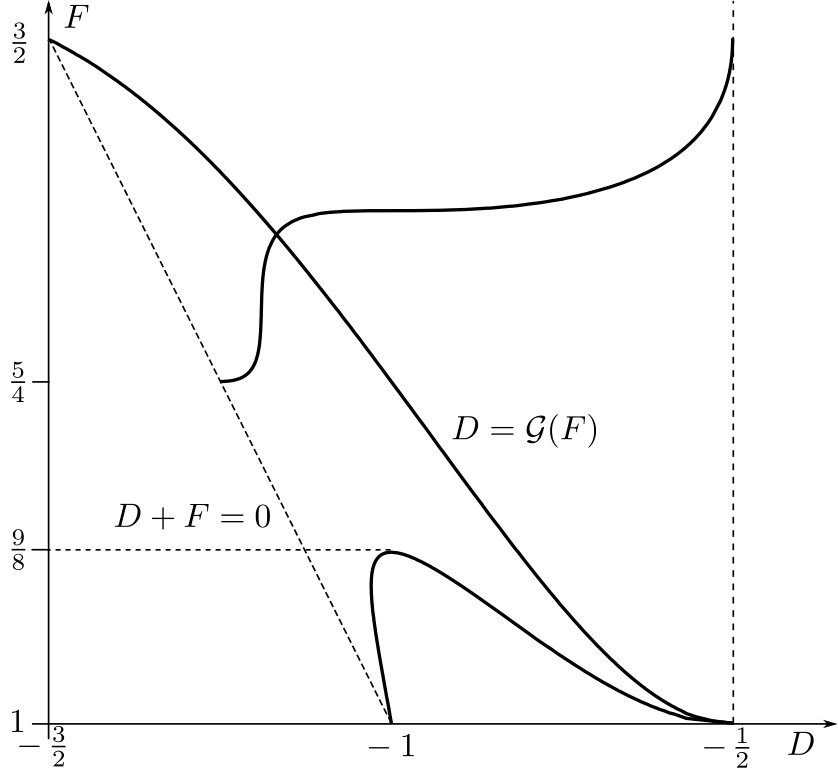 Figure 1
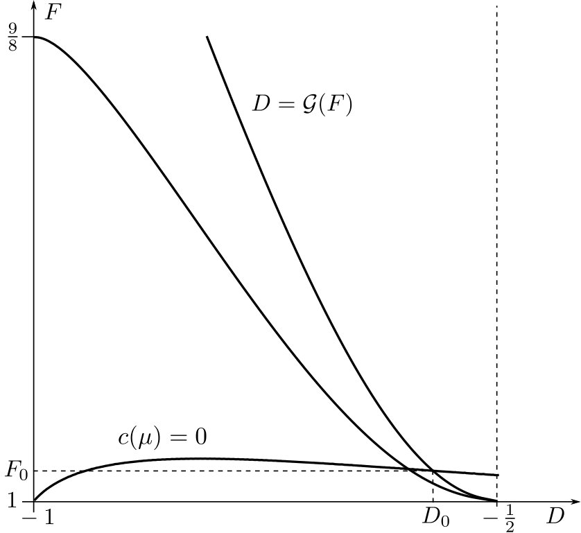 Figure 2
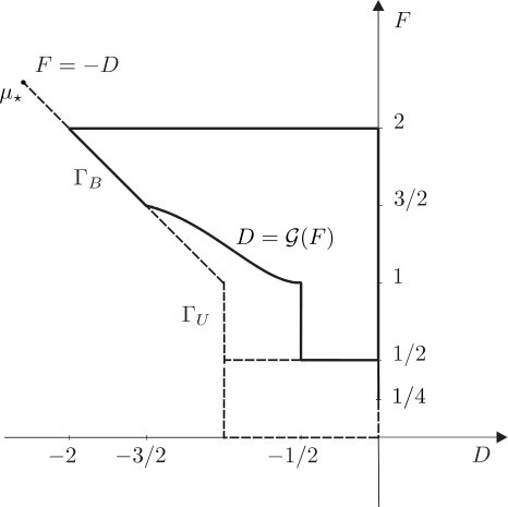 Figure 3
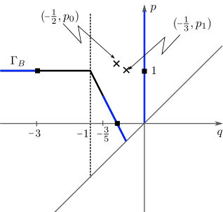 Figure 4
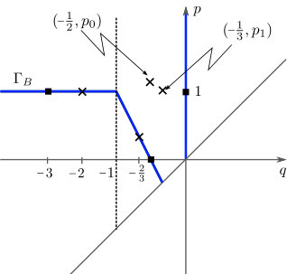 Figure 5
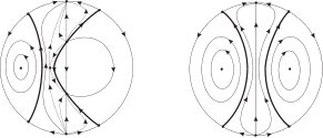 Figure 6
Peer Reviews
No public reviews on file for this paper yet. If you reviewed it on a platform where reviews are public (OpenReview, ICLR, NeurIPS, ICML), you can paste yours below so the community can read it here.
Videos
No videos yet. Explain this paper in a talk, walkthrough, or lecture? Add one.
Asymptotic development of an integral operator and boundedness of the criticality of potential centers
00footnotetext: 2010 Mathematics Subject Classification. 34C07; 34C23; 34C25. 00footnotetext: Key words and phrases: Center; Period function; Critical periodic orbit; Bifurcation; Criticality.
David Rojas
Departament d’Informàtica, Matemàtica Aplicada i Estadística,
Universitat de Girona, 17003 Girona, Spain.
Abstract
We study the asymptotic development at infinity of an integral operator. We use this development to give sufficient conditions to upper bound the number of critical periodic orbits that bifurcate from the outer boundary of the period function of planar potential centers. We apply the main results to two different families: the power-like potential family , , ; and the family of dehomogenized Loud’s centers.
1 Introduction
Consider a continuous family of planar potential systems
[TABLE]
where is a parameter, is an open subset of , , and is an analytic function defined in an open interval containing . In the case when and equation (1) has a non-degenerate center at the origin for each value of the parameter and so the point has a punctured neighbourhood that is entirely foliated by periodic orbits surrounding it. The largest neighbourhood with this property is the period annulus of the center and we shall denote it by . If we consider the embedding of into , its boundary, namely , is divided in two connected components: the origin itself, which is called the inner boundary of the period annulus, and the outer boundary of the period annulus defined by . When the center is a potential oscillator the natural parametrization of the closed orbits inside the period annulus is given by the energy level of the Hamiltonian . Since by convention, we have that , where denotes the energy level of the outer boundary .
The object under study in this paper is the period function of the center. The minimal period of the periodic orbit inside the energy level can be written as the Abelian integral
[TABLE]
This function is analytic on for each value of the parameter and it can be extended analytically to due to the non-degeneracy of the center. The derivative can also be written as an Abelian integral and its zeros correspond to critical periodic orbits of the system. This paper is concerned with the bifurcation of such critical periodic orbits from the outer boundary . That is, for a fixed , we aim to control the number of critical periodic orbits of system (1) that may emerge or disappear from as we move slightly the parameter . This number is called the criticality of the outer boundary.
- Definition 1.1.
Consider a continuous family of planar analytic vector fields with a center and fix some . Suppose that the outer boundary of the period annulus varies continuously at , meaning that for any there exists such that for all with . Then, setting
[TABLE]
the criticality of with respect to the deformation is \mathrm{Crit}\bigl{(}(\Pi_{\mu_{0}},X_{\mu_{0}}),X_{\mu}\bigr{)}\!:=\inf_{\delta,\varepsilon}N(\delta,\varepsilon).
In the previous definition stands for the Hausdorff distance between compact sets of . Notice that according with this definition the criticality may be infinite but, in the case it is not, it gives the maximal number of critical periodic orbits of tending to the outer boundary in the Hausdorff sense as the parameter approaches . The requirement of the continuity of with respect to the parameters of the system ensures that the possible changes of do not occur abruptly. We refer to [8] for details illustrating the necessity of this extra assumption.
- Definition 1.2.
A parameter is called a local regular value of the period function at the outer boundary of the period annulus if \mathrm{Crit}\bigl{(}(\Pi_{\mu_{0}},X_{\mu_{0}}),X_{\mu}\bigr{)}=0. Otherwise the parameter is called a local bifurcation value at the outer boundary.
The present paper is a contribution that follows the spirit of the series of works [5, 6, 15]. In these papers, we develop analytical tools which allow to give an upper bound of the criticality at the outer boundary of the period annulus of families of planar potential systems (1). The key idea is to find a collection of functions , , verifying that there exist such that form an Extended Complete Chebyshev system (ECT-system for short, see Definition 2) on the interval and . This fact implies that has at most zeros in , counting multiplicities, uniformly on the parameters . In particular, \mathrm{Crit}\bigl{(}(\Pi_{\mu_{0}},X_{\mu_{0}}),X_{\mu}\bigr{)}\leqslant n. According with Lemma 2.12, to give an upper bound of the criticality is reduced to guarantee that the Wronskian (see Definition 2) does not vanish for all . The tools of the previous works, and also the ones we present here, allow to tackle this problem in the following two situations: either or for all . That is, the case in which there exist and in any neighbourhood of with and is not considered.
Roughly speaking, the results in the previous papers relate the first term in the asymptotic development of the potential at the endpoints of with the first term of the asymptotic development of at . This allows to control the sign of the Wronskian under consideration for ; that is, uniformly on the parameters . However, there are some situations where these first terms of are not enough to compute the first term of the Wronskian at and so more terms in the asymptotic development must be employed. Theorem D and E in Section 3 aim to generalize the results in [5, 6, 15] in this direction. To accomplish the desired results, we will employ a generalization of [6, Proposition 2.16] and [15, Theorem D] (see Theorem C in Section 2.)
As an illustration of these generalizations we recover the study of two different families of planar centers. The first application is on the two-parametric family of potential differential system given by
[TABLE]
which has a non-degenerate center at the origin for all varying in . As far as we know, the period function of this center was originally studied by Miyamoto and Yagasaki [14], giving a monotonicity result for and . This result was improved later by Yagasaki [18] showing that the period function of (2) is monotonous for and any real. Motivated by those results, we considered the whole family (2) with and performed an exhaustive study of the period function in [7]. Concerning the criticality at the outer boundary, the family (2) became our testing ground for the techniques mentioned before. In these works, see Figure 1a, we proved that parameters \mu_{0}\in\Lambda\setminus\bigl{(}\Gamma_{B}\cup\{q+1=0\}\cup\{(-\tfrac{1}{2},p_{1})\}\cup\{(-\tfrac{1}{3},p_{2})\}\bigr{)}, with and , are local regular values of the period function at the outer boundary. In addition, \mathrm{Crit}\bigl{(}(\Pi_{\mu_{0}},X_{\mu_{0}}),X_{\mu}\bigr{)}\geqslant 1 if and it is exactly one for parameters satisfying either and , and , or and . Using the tools in the present paper, the bifurcation diagram in Figure 1a is improved by the following result. (See Figure 1b.)
Theorem A**.**
Let be the family of analytic potential systems (2) and consider the period function of the center at the origin. If with either and , or and then \mathrm{Crit}\bigl{(}(\Pi_{\mu_{0}},X_{\mu_{0}}),X_{\mu}\bigr{)}=1.
The proof of this result is presented in Section 4.1.1 (see Proposition 4.2) and Section 4.1.2 (see Proposition 4.6). The result finishes the bifurcation diagram of the period function at the outer boundary of the family (2) except for the line and four points in the parameter space. (See Figure 1b.) We point out that the line corresponds to parameters such that the energy at the outer boundary changes from infinite () to finite (). The points correspond to parameters that do not satisfy the technical hypothesis to apply the analytic tools. The bifurcation diagram in Figure 1b agrees with the global bifurcation diagram conjectured in [7].
The second application is on the family of quadratic polynomial planar centers. The literature classify quadratic centers in four families: Hamiltonian, reversible , codimension four , and generalized Lotka-Volterra . Chicone [2] conjectured that reversible centers have at most two critical periodic orbits whereas the centers of the other three families have monotonic period function. Regarding quadratic reversible centers, by an affine transformation and a constant rescaling of time, they can be brought to the Loud normal form
[TABLE]
In [3] the authors show that if the period of the center at the origin is globally monotone. When one can reduce the system, by means of a rescaling, to . That is,
[TABLE]
This family is known as dehomogenized Loud’s centers and it has a center at the origin for all parameters . The bifurcation of critical periodic orbits from the outer boundary of the period annulus of system (3) has been extensively studied in the recent years. (See Figure 2.) We refer to the series of papers [8, 10, 11, 12, 17, 16] and references therein.
Our contribution to the bifurcation diagram at the outer boundary of the dehomogenized Loud’s centers is to show that almost all parameters in the bifurcation curve have criticality exactly one. Up to now, this have been proved for parameters in that bifurcation curve with . In order to state the result properly, let us consider the parameter space
[TABLE]
Moreover, let be the Hypergeometric function (see [1, Section 15]), with and defined in (15), and let be the function in the statement of Lemma 4.3 using the expression of in (18).
Theorem B**.**
Let be the family of analytic potential systems (3) and consider the period function of the center at the origin. Let satisfying . Then \mathrm{Crit}\bigl{(}(\Pi_{\mu_{0}},X_{\mu_{0}}),X_{\mu}\bigr{)}=1 in the following situations:
If . 2.
If and . 3.
If , and
[TABLE]
The proof of the result is given in Sections 4.2.2 and 4.2.3. In that last Section, also a numerical manifestation that condition (4) seems to be fulfilled for is given. The condition is a technical requirement for the techniques involved in the proof and it is conjectured to be non necessary for the criticality to be also exactly one for those parameters satisfying . Regarding the equality we also show numerically that the equation has a unique solution in Section 4.2.3. The parameter is conjectured to have criticality exactly two at the outer boundary of the period annulus.
In the forthcoming paper [13] the authors also obtain (4) as a sufficient condition for bifurcation parameters in to have criticality exactly one using a completely different approach. In that work the authors study the asymptotic development of the Dulac time function near hyperbolic saddle singularities of meromorphic planar centers. They also use the dehomogenized Loud’s centers as testing ground and reach the same result in Theorem B without the technical restriction and allowing .
The rest of the paper is organized as follows. In Section 2 we study the asymptotic behaviour of an integral operator that will be useful for the proof of the dynamical results in the paper. In Section 3 we use these techniques to obtain two results that gives sufficient conditions in order to bound the criticality at the outer boundary of planar potential centers. Finally Section 4 is dedicated to the application of such sufficient conditions and so we prove Theorems A and B. The work is complemented with an Appendix that contain the more technical proofs.
2 Asymptotic behaviour of a certain integral operator
Let and consider the integral operator
[TABLE]
defined by
[TABLE]
Here, and in what follows, stands for the set of continuous functions on . In the collection of works [5, 6, 15] the previous operator is studied because of its relation with the bifurcation of critical periodic orbits. Indeed, the derivative of the period function of system (1) satisfies the equality
[TABLE]
with and . Roughly speaking, the main objective in these works is to give sufficient conditions to the first term of the asymptotic development at of the function in order that the first term of the asymptotic development at of is obtained, uniformly on the parameters. These conditions are formulated using the following notions.
- Definition 2.1.
Let be a continuous family of continuous functions on \bigl{(}a(\mu),b(\mu)\bigr{)}, meaning that the map is continuous on \bigl{\{}(x,\mu)\in\mathbb{R}\times\Lambda:x\in\bigl{(}a(\mu),b(\mu)\bigr{)}\bigr{\}}. Assume that either is continuous or in . Given we say that is continuously quantifiable in at by with limit if there exists an open neighbourhood of such that for all ,
If , then and . 2.
If , then and .
For the sake of shortness, in the first case we write at , and in the second case at . We use the analogous definition for the left endpoint .
We point out that the map in the previous definition is continuous at (see [5, Remark 2.6]).
From now on let us assume that . The purpose of this section is to deal with an specific situation that was not contemplated in the previous works. With this aim in view we first recover the main results in [5, 15].
- Definition 2.2.
The function defined for all and by means of
[TABLE]
is called the Roussarie-Ecalle compensator. For the sake of brevity, we also define
[TABLE]
where is the Gamma function. Following the notation in Definition 2, we write at if
[TABLE]
- Definition 2.3.
Let . We call
[TABLE]
the -th momentum of , whenever it is well defined. If we simply say that is the momentum of .
The next result gathers Theorems and in [5] together with Theorem C in [15].
Theorem 2.4**.**
Let be an open subset of and consider a continuous family of continuous functions on . Suppose that at . The following assertions hold:
If then at . 2.
If then at . 3.
If let us take such that . In this case:
If for and for some , then
[TABLE] 2.
If for and then
[TABLE] 3.
If for and then
[TABLE]
In the previous result the first term in the asymptotic development at infinity of the function is provided as soon as at except in the case when for some , , and for . In this special situation the hypothesis of to be quantifiable by is not enough to quantify at infinity. The following three functions exemplify this phenomena for even in the non-parametric scenario:
[TABLE]
All these functions are quantifiable by at infinity and it is a computation to show that their momenta vanish. One can verify that and are quantifiable at infinity by and respectively, and that
[TABLE]
These three examples subscribe the idea that more information on the asymptotic development of the function is needed to quantify in this situation. To address this problem we generalize Definition 2 as follows.
- Definition 2.5.
Let be a continuous family of continuous functions on . Assume that either is continuous or in . Given we say that has uniformly development at
[TABLE]
if there exists an open neighbourhood of such that for all ,
[TABLE]
for each . If then
[TABLE]
if for all ,
[TABLE]
We use the analogous definition at .
Similarly as in Definition 2, the functions are continuous at .
- Definition 2.6.
Let . Setting , we define
[TABLE]
for all .
The functions and \mathscr{F}\bigl{[}[f]_{m}\bigr{]} are related by the following result.
Lemma 2.7** (see [5]).**
Let . For any ,
[TABLE]
In the following statement the assumption in assertion is void in case that .
Proposition 2.8**.**
Let be a continuous family of continuous functions on satisfying at with positive integers and . The following holds:
If and with then, for
[TABLE]
and at . 2.
If then at .
- Proof.
We shall prove the result by induction on . To do so, we shall first assume . (In the case this assumption is void and we move to the next step.) Let us start considering . By definition of and elementary manipulations, we have
[TABLE]
for any . The hypothesis together with imply that the numerator of the second quotient tends to zero as tends to infinity. Therefore the second quotient is a -indeterminacy as for any . We apply the Uniform Hôpital’s Rule in [5, Proposition A.1] to deduce that
[TABLE]
for any . Similarly,
[TABLE]
Therefore,
[TABLE]
This proves the result for . If the result follows identically changing by . So we have
[TABLE]
for . Let us consider now that , and let us start by taking . The same procedure as before can be applied taking into account that the fist term in the asymptotic development disappear. Indeed, we have
[TABLE]
where now the sum starts at instead of the previous . Now using the first procedure the result follows for . Inductively the result holds for provided that . To finish the proof of , let us assume that . Then
[TABLE]
for all . Here we used that
[TABLE]
and, since , as . This proves . To show let us assume that . The procedure holds for all in this case. For all the terms in the asymptotic development associated with even powers disappear and so the only remaining term is the one with betas. Then,
[TABLE]
This ends the proof of the result.
- Remark 2.9.
A very useful tool for the computation of momenta was introduced in [5]. If is quantifiable by , with , and for then
[TABLE]
for some constant . We point out that this result do not contemplate the case when and for . Therefore this simplification can not be used in Proposition 2.8.
From now on, for the sake of simplicity, we shall assume that the functions are analytic on . The reason is that in Section 3 the differential system (1) is assumed to be analytic and so the functions involved also are. However, the reader may notice that weaker regularity is allowed in the forthcoming definitions and results. Let us recall at this point the notions of Chebyshev system and its relation with the Wronskian, which are both key ingredients for our purposes.
- Definition 2.10.
Let be analytic functions on an open real interval . The ordered set is an extended complete Chebyshev system (for short, a ECT-system) on if, for all , any nontrivial linear combination
[TABLE]
has at most isolated zeros on counted with multiplicities. (Let us mention that, in these abbreviations, “T” stands for Tchebycheff, which in some sources is the transcription of the Russian name Chebyshev).
- Definition 2.11.
Let be analytic functions on an open interval of . Then
[TABLE]
is the Wronskian of at .
These two notions are closely related by the following result (see for instance [4]).
Lemma 2.12**.**
* is an ECT-system on if and only if, for each ,*
[TABLE]
In the study of bifurcation of critical periodic orbits from the outer boundary the main objective is to bound the zeros of the derivative of the period function for energy levels uniformly on the parameters close to a fixed . Invoking equality (5), this problem is tackled by completing with a collection of analytic functions in order that form an ECT-system on for some and all . Note that guarantee the uniformity with respect to the parameters of the system is mandatory to obtain the desired upper bounds. With this aim in view, and on account of the characterization in Lemma 2.12, given , we consider the linear ordinary differential operator
[TABLE]
defined by
[TABLE]
Here, and in what follows, for the sake of shortness we use the notation . Furthermore we define in order that forthcoming statements contemplate the case as well. We also denote by the analytic functions on and by the functions on that can be extended analytically to .
Proposition 2.13** (See [6]).**
For any and , the following recurrence holds:
[TABLE]
where and for . In particular, if , then . Moreover, .
In the statement of the following result the assumptions in assertion and for in assertion are void in case that .
Theorem C**.**
Let be an open subset of and be a continuous family of analytic functions on . Assume that, in a neighbourhood of some fixed there exist continuous functions pairwise distinct at such that the function satisfies
[TABLE]
with positive integers and . The following holds:
If and for some then
[TABLE] 2.
If and then
[TABLE] 3.
If and then
[TABLE] 4.
If and , let us take such that and let us assume additionally that . In this case,
If for and for some , then
[TABLE] 2.
If for and then
[TABLE] 3.
If for and then
[TABLE]
- Proof.
Let us start by considering . In this case and the assumptions of Proposition 2.8 are satisfied. Moreover, if is satisfied then by in Proposition 2.8 we have
[TABLE]
Therefore, using Lemma 2.7 and Theorem 2.4 with , since ,
[TABLE]
This proves . Let us show , and . By hypothesis we have for . Therefore by in Proposition 2.8,
[TABLE]
The result follows using Theorem 2.4 with and Lemma 2.7 again. This ends the proof for the case .
Let us consider now . By Proposition 2.13 is an analytic function on for each and
[TABLE]
Then the result follows by applying the case to the family .
- Remark 2.14.
Let us recover at this point the examples in (6). The function satisfies the assumptions of Theorem C with , and . Since then assertion of the Theorem states that
[TABLE]
The function satisfies the hypothesis with , and . In this case and
[TABLE]
That is, satisfies the hypothesis in assertion of the Theorem with . Therefore,
[TABLE]
Finally, the function satisfies the hypothesis with , and . In this example assumptions in assertion are satisfied and
[TABLE]
We point out that Theorem C together with Theorem 2.4 cover all possible situations of the uniform asymptotic development of except the case when all powers are negative even numbers at . The last result of this Section is a recursive formula for the computation of a certain momentum that will be useful in the applications.
Lemma 2.15**.**
Let , and . Then,
[TABLE]
where and for .
- Proof.
By Definition 2 we have
[TABLE]
Using the recursive expression in Proposition 2.13,
[TABLE]
The result then follows integrating by parts.
3 Criticality of the period function at the outer boundary
In this section we apply Theorem C in order to obtain sufficient conditions to bound the number of critical periodic orbits that may bifurcate from the outer boundary of the period annulus in families of planar potential centers. We consider analytic differential systems (1) depending on a parameter and we assume that the origin is a non-degenerate center for all . We denote by the projection of the period annulus on the -axis, and by the energy level at the outer boundary of the period annulus.
- Definition 3.1.
We say that the family (1) verifies the hypothesis (H) in case that:
For all , the map is continuous on 2.
is continuous on or for all 3.
is continuous on or for all 4.
is continuous on or for all
Lemma 3.2** (See [5]).**
Let be a family of potential analytic differential systems verifying (H). Then the map is continuous on the open set \bigl{\{}(z,\mu)\in\mathbb{R}\times\Lambda:z\in\bigl{(}-\sqrt{h_{0}(\mu)},\sqrt{h_{0}(\mu)}\bigr{)}\bigr{\}}.
This section is divided in two parts according with the dichotomy produced by . First, Section 3.1 deals with the case . Second, Section 3.2 is dedicated to the case finite.
3.1 Potential systems with infinite energy
In this section we present sufficient conditions to bound the criticality at the outer boundary for potential systems satisfying for all . Following the strategy in [5, 6, 15], we find sufficient conditions such that can be embedded into the ECT-system , where is an analytic non-vanishing function. Next result is a combination of [6, Lemma 3.5] and [15, Lemma 3.3], and it is the key piece that connects the analytic tools studied in Section 2 with the dynamical results we are looking for.
Lemma 3.3**.**
Let be a family of potential analytic differential systems verifying (H) and such that . Assume that there exist continuous functions in a neighbourhood of some fixed , a continuous function with and an analytic non-vanishing function on such that
[TABLE]
with . Then \mathrm{Crit}\bigl{(}(\Pi_{\mu_{0}},X_{\mu_{0}}),X_{\mu}\bigr{)}\leqslant n-1.
The assumption requiring the existence of functions in the following statement is void in case that . The same happens to the assumptions in assertion and for in assertion in case that .
Theorem D**.**
Let be a family of potential analytic differential systems verifying (H) with and that there exist continuous functions in a neighbourhood of some fixed such that
[TABLE]
with positive integers and . Then \mathrm{Crit}\bigl{(}(\Pi_{\mu_{0}},X_{\mu_{0}}),X_{\mu}\bigr{)}\leqslant n if one of the following assertions hold:
If and for some . 2.
If and . 3.
If and , let us take such that . In this case:
If for and for some . 2.
If for .
- Proof.
For the sake of shortness let us denote . Lemma 3.2 and the hypothesis (H) imply that is a continuous family of analytic functions on . According to equality (5) the result will follow once we show that there exist in such a way has at most isolated zeros for and , multiplicities taken into account.
Let us assume that satisfies one of the hypothesis of the statement. Therefore satisfies one of the hypothesis in Theorem C, so we can assert that either
[TABLE]
or
[TABLE]
for some functions with and . Taking into account the definition of the operator , we have that either
[TABLE]
or
[TABLE]
Therefore, on account of equality (5), by Lemma 3.3 we have that \mathrm{Crit}\bigl{(}(\Pi_{\mu_{0}},X_{\mu_{0}}),X_{\mu}\bigr{)}\leqslant n as desired.
3.2 Potential systems with finite energy
We assume in this section that the energy at the outer boundary of system (1) is finite for all parameters . As in the previous works [5, 6, 15], in order to embed the function into some ECT-system for an appropriate non-vanishing function , the spirit of this section is to “translate” the case to the case so we can take advantage of Theorem C. This translation is given by the operator
[TABLE]
defined by
[TABLE]
where . Given , conjugates the operator with the linear ordinary differential operator
[TABLE]
defined by
[TABLE]
- Definition 3.4.
Let We call
[TABLE]
the -th momentum of , whenever it is well defined. If we simply say that is the momentum of .
Lemma 3.5**.**
Consider . Then the following hold:
* for * 2.
. 3.
\bigl{(}\mathscr{F}\circ\mathscr{B}\bigr{)}[f](x)=\sqrt{1+x^{2}}\bigl{(}\mathscr{B}\circ\mathscr{F}\bigr{)}[f](x)* for any * 4.
.
- Definition 3.6.
Given a continuous function on we define .
Lemma 3.7**.**
Let be a continuous family of analytic functions on . Then
[TABLE]
- Proof.
By definition with . Therefore, for a fixed ,
[TABLE]
Denoting , since as , we have that
[TABLE]
Consequently the result follows on account of Definition 2.
The following is an analogous version of Lemma 3.3 for the case finite. It gathers [6, Lemma 3.10] and [15, Lemma 3.8].
Lemma 3.8**.**
Let be a family of potential analytic differential systems verifying (H) and such that is continuous on . Assume that there exist continuous functions in a neighbourhood of some fixed , a continuous function with and an analytic non-vanishing function on such that
[TABLE]
with . Then \mathrm{Crit}\bigl{(}(\Pi_{\mu_{0}},X_{\mu_{0}}),X_{\mu}\bigr{)}\leqslant n-1.
In the same way as in the main result of the previous section, we stress that the assumption requiring the existence of functions in the following statement is void in case that . Also are void the assumptions in assertion and for in assertion in case that .
Theorem E**.**
Let be a family of potential analytic differential systems verifying (H) with for all and that there exist continuous functions in a neighbourhood of some fixed such that the function
[TABLE]
satisfies
[TABLE]
with integers and . Then \mathrm{Crit}\bigl{(}(\Pi_{\mu_{0}},X_{\mu_{0}}),X_{\mu}\bigr{)}\leqslant n if one of the following assertions hold:
If and for some . 2.
If and . 3.
If and , let us take such that . In this case:
If for and for some . 2.
If for .
- Proof.
According with Lemma 3.2 and the hypothesis (H), the family is a continuous family of analytic functions on . On account of equality (5), after the appropriate rescaling,
[TABLE]
Therefore the result will follow if there exist and a neighbourhood of such that has at most zeros for all and , multiplicities taken into account. To this end, we shall use that the operator commutes the linear differential operators , defined for functions in , with , defined for functions in . Then, as we proceeded in Theorem D, we aim to apply Theorem C in this case to the family .
First, by hypothesis we have that
[TABLE]
so, on account of Lemmas 3.5 and 3.7, we have
[TABLE]
Moreover, on account of Lemma 3.5 and Definition 3.2,
[TABLE]
That is,
[TABLE]
Therefore, if satisfies one of the hypothesis of the statement, the function satisfies one of the hypothesis in Theorem C. It turns out then that either
[TABLE]
or
[TABLE]
for some functions with and . Let us note that
[TABLE]
with , where we use in Lemma 3.5 in the first quality, the identity with in the second equality, and in Lemma 3.5 in the third equality. So we have
[TABLE]
with . Using the definition of , the previous equation yields to
[TABLE]
Setting , the previous identity implies that
[TABLE]
Thus, on account of the definition of in (8),
[TABLE]
which, since , implies that
[TABLE]
with and . The result follows then by Lemma 3.8 and taking the identity (9) into account.
4 Applications
In this Section we present the results obtained applying Theorems D and E to the two-parametric families of centers introduced in Section 1.
4.1 The family
The family of vector fields (2) is an analytic potential system with potential function
[TABLE]
According with the dichotomy that produces in hypothesis (H), in order to prove Theorem A we split the parameter space in two parts: and . As mentioned in the Introduction, the line correspond to parameters such that in any neighbourhood of them and coexist. This scenario is out of reach with the current techniques. If system (2) has a non-degenerate center at the origin and the projection of the period annulus on the -axis is with \rho(\mu)\!:=\bigl{(}\tfrac{p+1}{q+1}\bigr{)}^{\frac{1}{p-q}}. Moreover, the energy at the outer boundary is for all . On the other hand, if the origin is also a non-degenerate center but in this case and . (For more details in this direction we refer to [7].) In particular, in both cases hypothesis (H) in Definition 3 is fulfilled. The proof of Theorem A follows directly from Propositions 4.2 and 4.6.
4.1.1 The criticality is at most one in
The purpose of this Section is to apply Theorem D with on family (2) to parameters with , . According with the Theorem, we first need to compute the asymptotic expression of the function at . To this end, we follow the same strategy used on the proof of [6, Theorem A]. Since the function is analytic on , we can write
[TABLE]
for all . On account of the equalities with and , equality (11) reads
[TABLE]
where
[TABLE]
Lemma 4.1**.**
Let be defined as above with defined in (10). Taking , the following hold:
* at .* 2.
* at .*
- Proof.
By means of some algebraic manipulations the function writes
[TABLE]
where . Using the expression in (10) we can assert that is the sum of monomials of the form with for and a well defined rational function at . The biggest exponent for is with coefficient . Let us notice that, since the coefficient vanishes at , is not continuously quantifiable at infinity in unless we fix . With this choice of , the following two largest exponents for are and . More precisely, we have
[TABLE]
The result in follows using that as and . The assertion follows similarly now looking for the smallest exponent for .
Proposition 4.2**.**
Let be the family of analytic potential systems (2) and consider the period function of the center at the origin. If with then \mathrm{Crit}\bigl{(}(\Pi_{\mu_{0}},X_{\mu_{0}}),X_{\mu}\bigr{)}=1.
- Proof.
From [5] we already know that \mathrm{Crit}\bigl{(}(\Pi_{\mu_{0}},X_{\mu_{0}}),X_{\mu}\bigr{)}\geqslant 1. Let us prove the opposite inequality. According with equality (12) and Lemma 4.1, the function satisfies
[TABLE]
at , where
[TABLE]
and
[TABLE]
We point out that is continuous but changes sign at . On account of the previous computations, the quantifier at infinity of at is . In addition, the first momentum on Theorem D vanishes identically. Indeed,
[TABLE]
for all . Moreover, and is continuous for . Therefore, condition in Theorem D holds. This proves that the criticality at is at most one.
4.1.2 The criticality is at most one in
The energy at the outer boundary of the period annulus for parameters is finite. Accordingly we shall use Theorem E with to parameters with , in order to prove the second assertion of in Theorem A. A similar argument as in the previous section shows that
[TABLE]
where
[TABLE]
Here, and in what follows, we omit the dependence in of for the sake of simplicity. Next result is general for any potential function with finite energy at the outer boundary.
Lemma 4.3**.**
Let be defined as above and fix . Assume that, for all in a neighbourhood of , is finite and the right endpoint of the projection of the period annulus is also finite and satisfies . Then
[TABLE]
with
[TABLE]
The analogous result is true for .
- Proof.
The function can be written, after some algebraic manipulations, as
[TABLE]
where \psi\!:=-\bigl{(}(V^{\prime})^{2}-2VV^{\prime\prime}\bigr{)}\bigl{(}(V^{\prime})^{2}(h_{0}(\nu-1)+3V)+6(h_{0}-V)VV^{\prime\prime}\bigr{)}-4V^{2}(h_{0}-V)V^{\prime}V^{\prime\prime\prime}. Since the function is analytic at the result follows by considering the Taylor’s expansion at of the previous expression and using the change of variable .
Lemma 4.4**.**
Let be defined as above with defined in (10). Taking and with and then
[TABLE]
Moreover, the asymptotic expression in Lemma 4.3 holds with .
- Proof.
The first assertion of the result can be proven similarly as Lemma 4.1 so we skip the details for the sake or brevity. We only prove that . Indeed, using the expression in (10) and substituting some tedious but elementary computations show that (see Lemma 4.3)
[TABLE]
We stress that each term inside the parenthesis is positive for . Also the multiplicative term is non-vanishing so .
The following result is the version of [6, Lemma 3.12] for .
Lemma 4.5**.**
Let and . Let us assume that is quantifiable at by . If then
[TABLE]
Proposition 4.6**.**
Let be the family of analytic potential systems (2) and consider the period function of the center at the origin. If with and then \mathrm{Crit}\bigl{(}(\Pi_{\mu_{0}},X_{\mu_{0}}),X_{\mu}\bigr{)}=1.
- Proof.
From [5] we already know that \mathrm{Crit}\bigl{(}(\Pi_{\mu_{0}},X_{\mu_{0}}),X_{\mu}\bigr{)}\geqslant 1. Let us prove the opposite inequality. Let us denote for the sake of simplicity. In [6, Lemma 4.4] it was shown that satisfies the hypothesis on Lemma 4.5 for all . Applying Lemma 4.5 with we have then N\bigl{[}\mathscr{D}_{\nu(\mu)}[f_{\mu}]\bigr{]}=0 for all . Moreover, on account of the equality (13) and Lemma 4.4,
[TABLE]
where
[TABLE]
and
[TABLE]
due to by Lemma 4.4. Let us apply now Theorem E with . According with the previous discussion, if and then assertion in of Theorem E is satisfied with , and due to N\bigl{[}\mathscr{D}_{\nu(\mu)}[f_{\mu}(z)]\bigr{]}\equiv 0 and . Then \mathrm{Crit}\bigl{(}(\Pi_{\mu_{0}},X_{\mu_{0}}),X_{\mu}\bigr{)}\leqslant 1 in this case. On the other hand, if we apply Theorem E with , and . By Lemma 5.4 we also have
[TABLE]
Then assertion in Theorem E states that \mathrm{Crit}\bigl{(}(\Pi_{\mu_{0}},X_{\mu_{0}}),X_{\mu}\bigr{)}\leqslant 1 also in this case.
4.2 The family of dehomogenized Loud’s centers
Through all this section we consider parameters inside the open set
[TABLE]
The Loud system (3) has a first integral given by
[TABLE]
for all (see for instance [11]) where with
[TABLE]
and integrating factor . The line at infinity , the line and the conic are invariant curves of the differential system and, for parameters , is a hyperbola intersecting the -axis at
[TABLE]
with . The outer boundary of the period annulus of the center at the origin of system (3) consists of the branch of the hyperbola passing through and the line at infinity , joined by two hyperbolic saddles (see Figure 3.) Although it is not relevant at this moment (but it will be nearly soon) we point out that there is a bifurcation on the phase portrait at due to the fact that the branch of hyperbola passing through crosses the invariant line . In particular, if and only if .
In [11] the authors give an implicit expression of the bifurcation curve in . More concretely, for each and small let be the period of the periodic orbit of system (3) passing through the point . Then, for parameters in , the derivative of the period function tends to as tends to zero uniformly on compact subsets of , where
[TABLE]
The bifurcation curve is given by the zero set of and the following properties are deduced:
for all . 2.
, and 3.
.
For the proof of these results we refer to [11, Theorem 3.6 and Proposition 3.11]. In particular the curve is analytic on and joins the parameters and . The following result gives a more compact expression of the zero set of and an additional property. The proof is given in the Appendix.
Proposition 4.7**.**
For parameters the zero sets of and \tfrac{1}{\Gamma\bigl{(}\tfrac{7}{2}-4F\bigr{)}}{}_{2}F_{1}\left(-\tfrac{1}{2},\tfrac{3}{2};\tfrac{5}{2}-2F;\tfrac{p_{2}-1}{p_{2}-p_{1}}\right) coincide. Moreover, .
The Loud system (3) is not a potential system and, at first glance, is not suitable to use the techniques developed in this paper to study the criticality at the outer boundary of its center. However we recall that it has a first integral quadratic in and its integrating factor depends only on . These two properties are the requirements of [3, Lemma 14], which shows that the change of variables
[TABLE]
transforms system (3) to the potential system
[TABLE]
The potential system above has a non-degenerated center at the origin and all the properties that we derive of its period function are directly transmitted to the period function of the Loud’s center. In these new variables, the projection of the period annulus is , where
[TABLE]
Let by the Hamiltonian function associated to system (16) with . If we set the following expressions will be useful to simplify the forthcoming computations:
[TABLE]
Here denotes the energy of the outer boundary of the center for all . In particular, is finite in .
4.2.1 Quantification of the functions involved
With the aim of applying Theorem E with to parameters satisfying , we need to compute the first terms of the asymptotic development of at . We recall that the previous is reduced to study the asymptotic development of
[TABLE]
at and due to equality (13). Here, and in what follows, we omit the dependence in of and for the sake of brevity. Moreover we use instead of to be consistent with the notation in (16).
Lemma 4.8**.**
Let and be defined as above. Taking we have that
[TABLE]
where
[TABLE]
- Proof.
In order to get the desired asymptotic expression of S_{\mu}\bigl{(}g_{\mu}^{-1}(-z\sqrt{h_{0}})\bigr{)} at we study the asymptotic expression of at . The result will follow then on account of the change of variable . To do so we invoke the expression in (14) and perform the change of variable . Taking advantage of the relations in (18) we can write in terms of the polynomials and some powers of depending on the parameter . Due to the fact that as , we are concerned about the asymptotic expression of at . An analogous study than the one done in Lemma 4.1 shows in this case that
[TABLE]
The result follows undoing the change of variable.
4.2.2 Proof of Theorem B
From the results in [11] we already know that \mathrm{Crit}\bigl{(}(\Pi_{\mu_{0}},X_{\mu_{0}}),X_{\mu}\bigr{)}\geqslant 1 for parameters satisfying . The strategy for showing the opposite inequality is to apply Theorem E with to the family (16). To do so, let be defined as in the statement of the Theorem. The first thing to notice is that satisfies hypothesis (H) with for all . Let us fix . On account of equality (13) and Lemmas 4.3 and 4.8 we have that
[TABLE]
where
[TABLE]
and
[TABLE]
If then and assertion in Theorem E is fulfilled with , and . Therefore, assertion in Theorem B holds.
If then . Let us split this interval in two parts, namely and . The parameter is excluded due to the noncontinuity of the function . If then the coefficient of in the previous asymptotic expansion is the nonvanishing function on Lemma 4.8. Moreover, by Lemma 4.5, for all . Consequently, we apply Theorem E with , and . Using Lemma 5.5 we have that
[TABLE]
Proposition 4.9 ensures that the previous Hypergeometric function do not vanishes for . Consequently, hypothesis of Theorem E are fulfilled and so the criticality at the outer boundary for those parameters is exactly one.
Let us finally consider . In this case the coefficient of on the asymptotic expansion above is given in Lemma 4.3. Here then we invoke the assumption in the statement of Theorem B regarding . As before we can apply Theorem E with , and and the hypothesis are satisfied whenever condition (4) is fulfilled. That is, whenever the hypergeometric function above do not vanish. Again Proposition 4.9 ensures that this is true for parameters . Consequently, the result in assertion of Theorem (B) holds. For parameters condition (4) is required and so the result follows if it is satisfied. This ends the proof of the first assertion in Theorem B.
4.2.3 Some additional comments
This section is devoted to discuss some technicalities involved in the proof of Theorem B. More concretely, we show that condition (4) is fulfilled when and we also give some numerical intuition to the fact that the condition should be fulfilled for every .
Proposition 4.9**.**
If satisfy with then
[TABLE]
- Proof.
From the fact that the parameters satisfy with it follows that and so . Moreover . Consequently, .
Consider the function
[TABLE]
From [1] the derivative of with respect to writes
[TABLE]
Using the series expression of the Hypergeometric function it turns out that all its coefficients are positive for . Consequently, for each we have that
[TABLE]
Hence for each the function is increasing for . In addition,
[TABLE]
if . Therefore, for each , the function is positive for all . Taking and on account of for all parameters under consideration, the result follows.
Figure 4a exhibits the curve together with the two connected components of the zero set level of the function
[TABLE]
As the previous result states, there is no crossing of the zero set with the curve for parameters with . Indeed Proposition 4.9 shows that condition (4) is satisfied in this situation. Numerics seems to show that the non-crossing property is still verified till . However, we have not been able to prove it analytically.
We end this section with also a numerical intuition about the equation in the statement of Theorem B. Although again no analytical prove is provided, it seems that this equation has a unique solution with is approximately .
5 Appendix: Computation of momenta
The purpose of this section is to compute the momenta used to apply Theorem E on the two-parametric potential family and the Loud’s family (see Proposition 4.6 and Section 4.2.2.) In both cases the momentum we are interested in is
[TABLE]
Lemma 3.5 together with Definition 3.2 imply that
[TABLE]
Using the formula in Lemma 2.15 on the right-hand side of the equality above, we get the equality
[TABLE]
Finally, the change of variable yields to
[TABLE]
Let with . In both families, for parameters under consideration the momentum vanishes. We point out that this fact is not a coincidence. Indeed, in both cases we are interested to bound the criticality of bifurcation parameters such that In other words, the bifurcation occurs in such a way that is convergent for all and changes sign at . From the definition of the period function, it turns out that
[TABLE]
and so we have (we refer to [5, Corollary 3.12] for more details in this direction.) Hence, for parameters in such situation,
[TABLE]
Next two lemmas are useful for the forthcoming computations. See for instance and of [1] for the first one. The first assertion of the second lemma was proved in [5, Lemma A.3]. The second assertion follows similarly.
Lemma 5.1**.**
Let and be any complex numbers with strictly positive real part. Then
[TABLE]
where denotes the Gamma function.
Lemma 5.2**.**
Let and be real numbers such that . Then
[TABLE]
and
[TABLE]
Lemma 5.3**.**
Let . The following hold:
If with is defined by (10) and then
[TABLE]
and
[TABLE]
where , , and . 2.
If with is defined by (18) then
[TABLE]
and
[TABLE]
where , and , are defined in (15).
- Proof.
Let us compute the integrals in . Using the expression of in (10) we have that
[TABLE]
We perform the change of variable . Then the integral above writes
[TABLE]
where . This improper integral is divergent as tends to \rho=\bigl{(}\frac{p+1}{q+1}\bigr{)}^{\frac{1}{p-q}}, which will be the case under consideration. We shall make explicit the order of the singularity of this function using Lemma 5.1. In order to apply it, we note that the power of in the integrand should be greater than and the power of negative. The first condition is satisfied for , , but is positive for some parameters. (In fact vanishes for the bifurcation parameters.) To overpass this situation, we apply Lemma 5.2, getting
[TABLE]
Using we can write and so,
[TABLE]
as desired. Similarly we can obtain the expression for the second integral in . In this case, we need to apply Lemma 5.2 twice in order that the power of of the integrand is negative. We omit the details for the sake of brevity.
Let us now prove . Using the expression of in (18) together with the change of variable the first integral on item is written as
[TABLE]
By definition of and in (15) the difference on the integrand above decomposes as
[TABLE]
Let us now consider the change of variable In this new variable, we have that
[TABLE]
with . As in , we point out here that tends to zero as tends to (see (17)) which will be the case under study. In particular, the above improper integral is divergent as tends to zero. To deal with this situation, we add and subtract the value at of inside the integral, which turns out to be exactly . That is,
[TABLE]
as desired. Similarly we obtain the expression for the second integral in . In this case, we need to add and subtract to the function , which turns out to be its Taylor’s development up to degree one.
Lemma 5.4**.**
Let be defined as in (10) and . If with and then
[TABLE]
- Proof.
For the parameters under consideration the equality deduced in (21) holds. For the sake of simplicity we shall omit the dependence on the parameter from now on. We stress that although the dependence on the parameters is not shown all the limits in the proof are uniform with respect to the parameters. Using the definition of , that is
[TABLE]
with , and the change of variable , the following equality holds
[TABLE]
with . The function tends to zero as . Moreover, has a singularity at of order , which is integrable since . Consequently,
[TABLE]
Let us define
[TABLE]
We have . Denoting and integrating by parts, the previous discussion leads to the equality
[TABLE]
Here we used that , which is a direct computation. By definition,
[TABLE]
Then,
[TABLE]
From now on let us denote . Using the expressions of and we have
[TABLE]
Substituting (24) and the integrals in assertion of Lemma 5.3 into (23), and taking into account that
[TABLE]
we obtain
[TABLE]
Let us now compute . Using again the expression of the previous function writes
[TABLE]
First, the change of variable on the second quotient of the previous equality yields to
[TABLE]
The function as and the function in the right hand side of the previous equality has a singularity at of order . Since we have that
[TABLE]
Second, the change of variable yields to the same expression as before,
[TABLE]
On account of the expression of , expanding in series on we have that
[TABLE]
Let us recall . At this point we claim that
[TABLE]
Indeed, the previous expression writes
[TABLE]
Using the expression of and appearing in Lemma 5.3,
[TABLE]
for some . Substituting the previous equality on the limit above and taking into account that as the claim follows. Therefore,
[TABLE]
Let us now fix . On account of the expression of we have that . Finally, using the expressions of and , the fact that as and Lemma 5.1 we obtain
[TABLE]
as we desired.
Lemma 5.5**.**
Let be defined as in (18). The following holds:
If satisfies , and then
[TABLE] 2.
If satisfies and then
[TABLE]
Here , and , are defined in (15).
- Proof.
The proof of the assertion in follows the same lines as the proof of using that
[TABLE]
Since the proof of is richer in subtle technicalities, and for the sake of brevity, we decided to prove and omit the proof of assertion in .
Let us show . For the parameters with the equality in (21) holds. Again we omit the dependence on parameters for the sake of simplicity although all the limits are uniform with respect to the parameters. Following the same discussion as in the proof of Lemma 5.4 we arrive to the equality
[TABLE]
where the functions , and are defined in (22). The only difference lies on the interval of integration due to as in this case.
Let us denote From the expressions of and in (22) and the definition of and in (18) we have
[TABLE]
Moreover, equality (26) also holds and the limit of the second quotient of the right-hand side of the equality tends to zero as tends to one. Therefore
[TABLE]
The change of variable yields to
[TABLE]
On account of the expressions in (18), if we have
[TABLE]
Finally, using the factorization and defined above, after some algebraic manipulations we arrive to
[TABLE]
At this point we substitute the previous equality and (27) into (21), and we use the equality (28) and the integrals in item of Lemma 5.3 to have an explicit expression for the momentum under consideration. On account that (see Lemma 5.3), we can collect the expression of the momentum as follows
[TABLE]
where
[TABLE]
and both and are analytic functions at . Here . First, from the first part of the proof of Lemma 4.6 we know that N\!\left[\bigl{[}\mathscr{D}_{\nu}[f_{\mu}]\bigr{]}^{1}\right] exists and so the previous limit is finite. (This can also be deduced from the fact that at the moment when certain momentum in Theorem E needs to be computed, such momentum exists and it is finite.) The previous fact, together with the analyticity of and , implies that as . Second, we point out that is the expression of the curve found in [11] which vanishes for bifurcation parameters we are considering. Consequently, taking the limit on the equality above,
[TABLE]
The result will follow once we prove that
[TABLE]
To do so we shall show that the power series of the functions at both sides of the equality coincides. We notice that for parameters under consideration, and so the Hypergeometric function is analytic and well defined as a power series (see [1, Section 15]). First notice that using the Newton’s binomial the integrand of writes
[TABLE]
By the assertion in Lemma 5.1 and on account that , for each we have
[TABLE]
Since the function inside the integral is positive for each , Tonelli’s theorem states that summation and integral signs interchange. Thus we obtain
[TABLE]
Let us now integrate the second term in (29). The integration of the first term follows similarly and we omit the computation for the sake of shortness. Taking small we have
[TABLE]
With the aim of applying Lemma 5.1 in view we need the powers of and to be greater than . Indeed, since we already have . On the contrary, the power of do not satisfy the assumptions of the lemma. To overcome this we use Lemma 5.2 and we get
[TABLE]
Substituting this equality on the previous expression, tending to zero and using Lemma 5.1 we get
[TABLE]
As we noticed before, the same procedure shows that
[TABLE]
In this last case Lemma 5.2 must be applied twice. Summing these two last expressions together with (30) we have that
[TABLE]
where on the first equality we use common properties of the Gamma function and on the second equality we use the definition of the Hypergeometric function as a power series on account that .
- Remark 5.6.
The Hypergeometric function {}_{2}F_{1}\bigl{(}a,b;c;z) can be continued analytically for any complex number with along any path in the complex plane that avoids the branch points 1 and infinity. For parameters satisfying , and the property do not hold. However, it holds that . Thus the function
[TABLE]
in the statement of Lemma 5.5 is well defined as a power series.
- Proof of Proposition 4.7
As it is shown in (20) the bifurcation curve must coincide with the zero set of . For the parameters under consideration, the first assertion in Lemma 5.5 shows that this zero set coincide with the zero set of the function {}_{2}F_{1}\bigl{(}\tfrac{3}{2},-\tfrac{1}{2};\tfrac{5}{2}-2F;\alpha) where . This proves the first assertion of the result. To show the second assertion notice that
[TABLE]
since as . Therefore the result follows by the limit \lim_{(D,F)\rightarrow(-1,5/4)}\frac{\Gamma(3-2F)}{\Gamma\bigl{(}\tfrac{5}{2}-2F\bigr{)}}=0.
Acknowledgements
The author thanks D. Marin and J. Villadelprat for fruitful discussions and valuable comments during the development of this work. The author is partially supported by the MINECO/FEDER grant MTM2017-82348-C2-1-P and the MINECO/FEDER grant MTM2017-86795-C3-1-P.
The reference list from the paper itself. Each links out to its DOI / PubMed record.
- 1[1] M. Abramowitz, I. Stegun. Handbook of Mathematical Functions with Formulas, Graphs, and Mathematical Tables . Dover Publications, 1965.
- 2[2] C. Chicone. Review in Math Sci Net. Ref. 94h:58072.
- 3[3] A. Gasull, A. Guillamon, J. Villadelprat. The period function for second-order quadratic OD Es is monotone. Qual. Theory Dyn. Syst. 5 (2004) 201–224.
- 4[4] S. Karlin, W.J. Studden. Tchebycheff systems: With applications in analysis and statistics. Pure and Applied Mathematics, Vol. XV. Interscience Publishers John Wiley & Sons, New York-London-Sydney (1996).
- 5[5] F. Mañosas, D. Rojas, J. Villadelprat. The criticality of centers of potentials systems at the outer boundary. J. Differential Equations 260 (2016) 4918–4972.
- 6[6] F. Mañosas, D. Rojas, J. Villadelprat. Analytic tools to bound the criticality at the outer boundary of the period annulus. J. Dynamics and Differential Equations (2016) 1–27.
- 7[7] F. Mañosas, D. Rojas, J. Villadelprat. Study of the period function of a two-parameter family of centers. J. Math. Anal. Appl. 452 (2017) 188–208.
- 8[8] F. Mañosas, J. Villadelprat. A note on the critical periods of potential systems. Int. J. Bifur. Chaos Appl. Sci. Eng. 16 (2006) 765–774.