
TL;DR
This paper investigates the size of minors in expander graphs, establishing bounds on the largest minor size, and provides algorithms for embedding specific minors, advancing understanding of minor-rich properties in expanders.
Contribution
It introduces a new lower bound on the size of minors in expanders and offers an efficient randomized algorithm for finding such minors, improving upon previous results.
Findings
Established a lower bound for minors in expanders proportional to n/(log n)
Provided a randomized algorithm to find minors of size up to that bound
Showed expanders are the most minor-rich graphs in a certain sense
Abstract
In this paper we study expander graphs and their minors. Specifically, we attempt to answer the following question: what is the largest function , such that every -vertex -expander with maximum vertex degree at most contains {\bf every} graph with at most edges and vertices as a minor? Our main result is that there is some universal constant , such that . This bound achieves a tight dependence on : it is well known that there are bounded-degree -vertex expanders, that do not contain any grid with vertices and edges as a minor. The best previous result showed that , where depends on both and . Additionally, we provide a randomized algorithm, that, given an -vertex…
Click any figure to enlarge with its caption.
 Figure 1
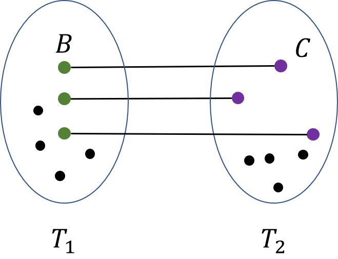 Figure 2
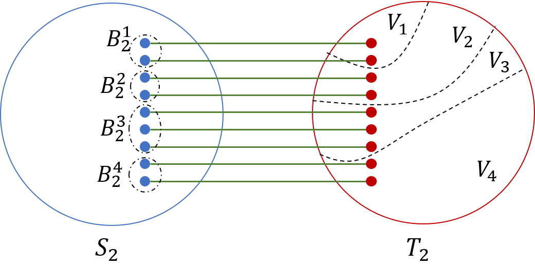 Figure 3
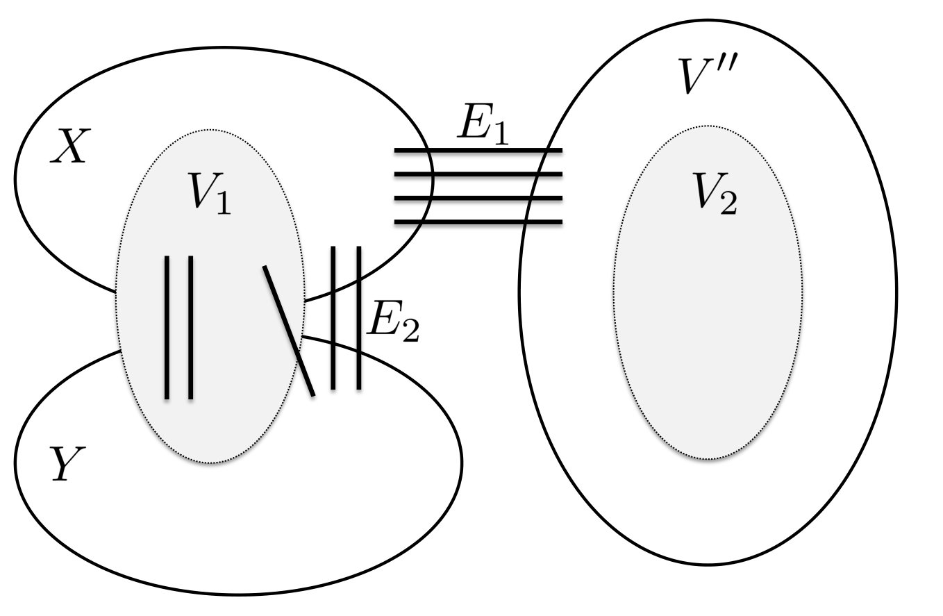 Figure 4
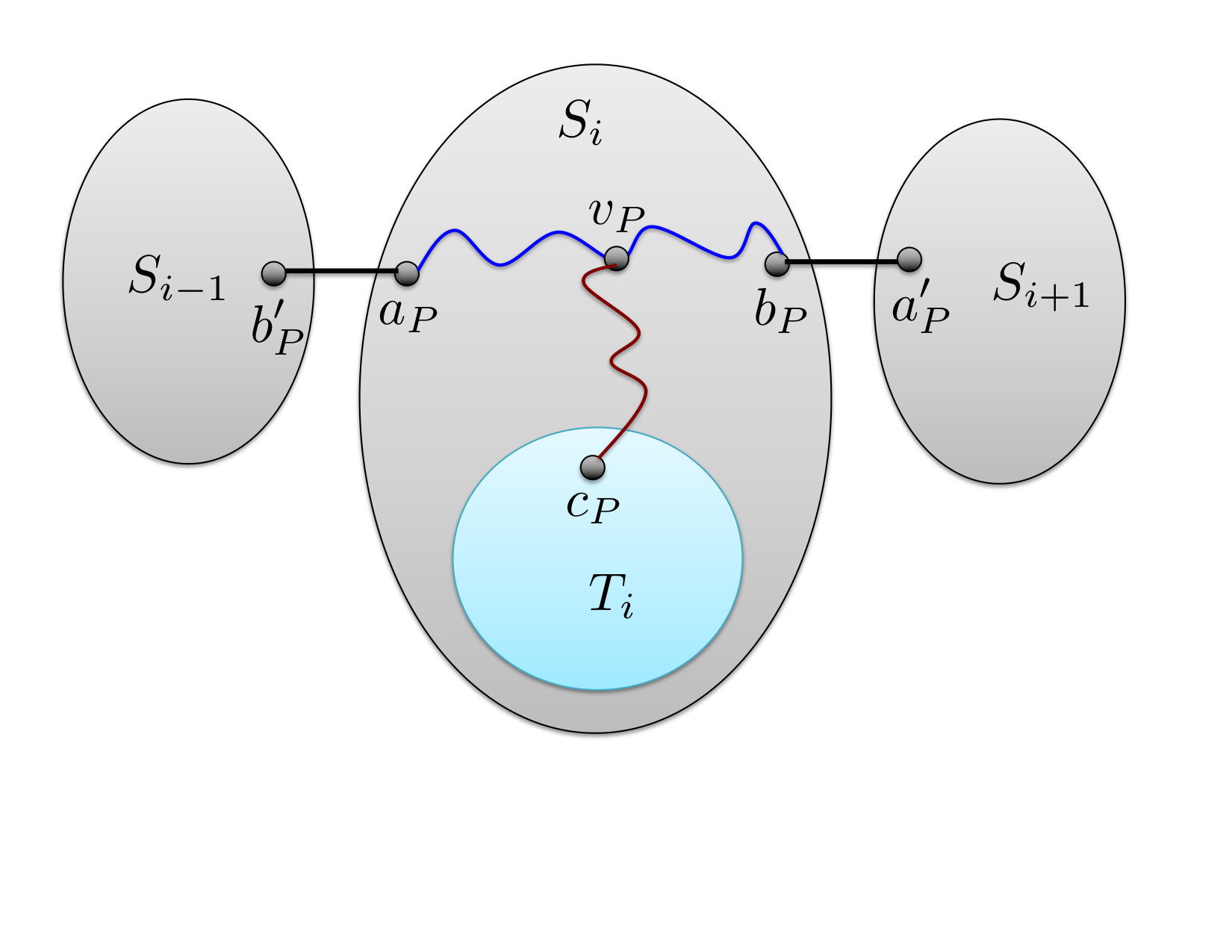 Figure 5
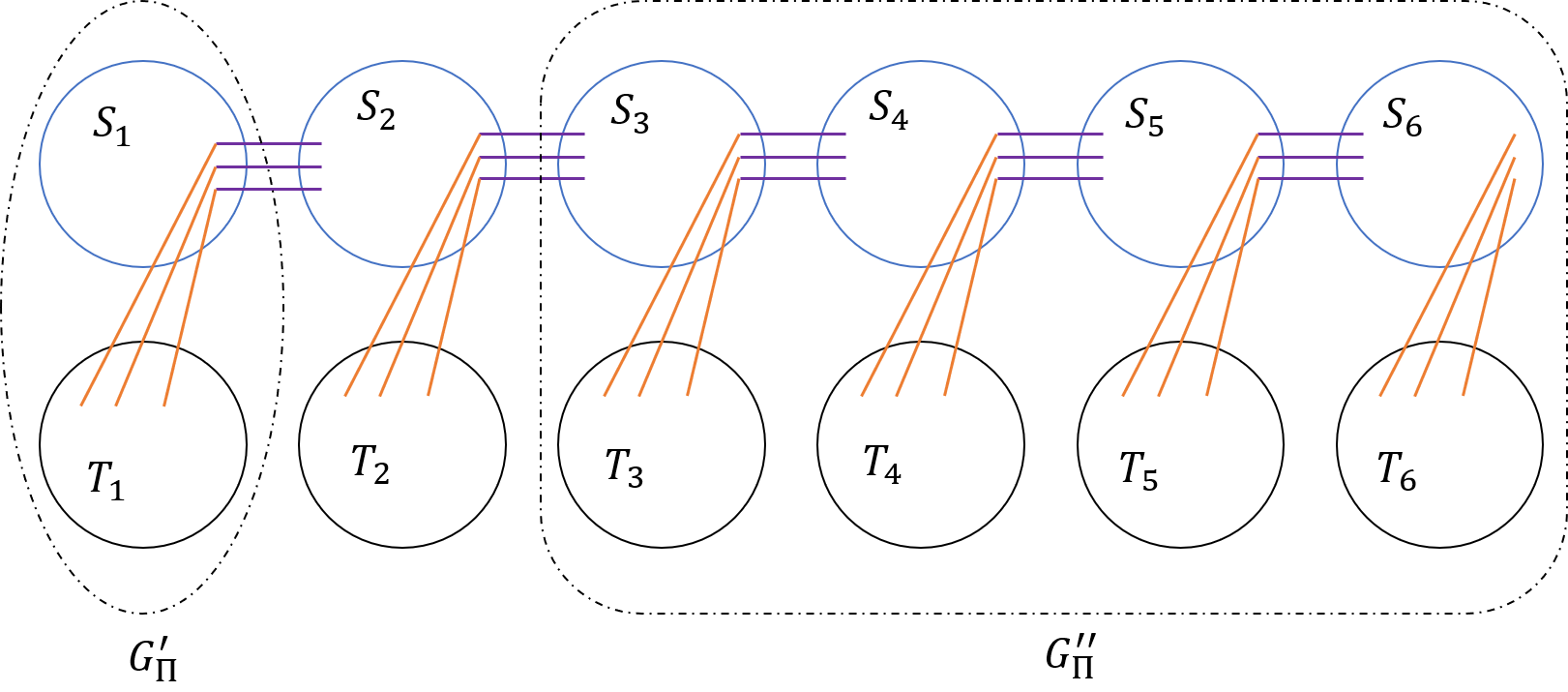 Figure 6
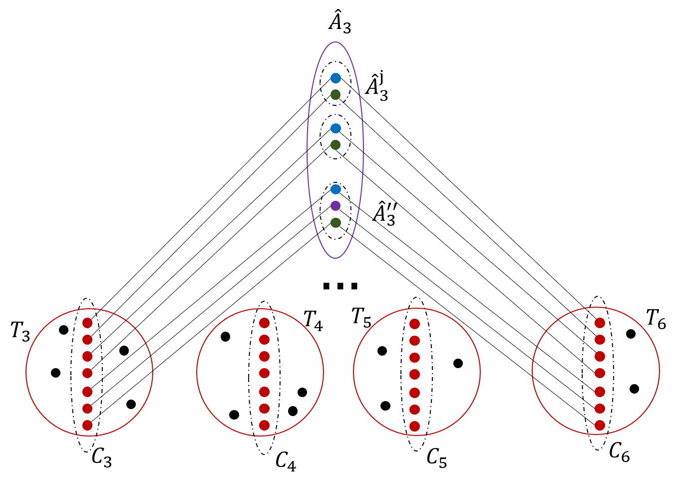 Figure 7
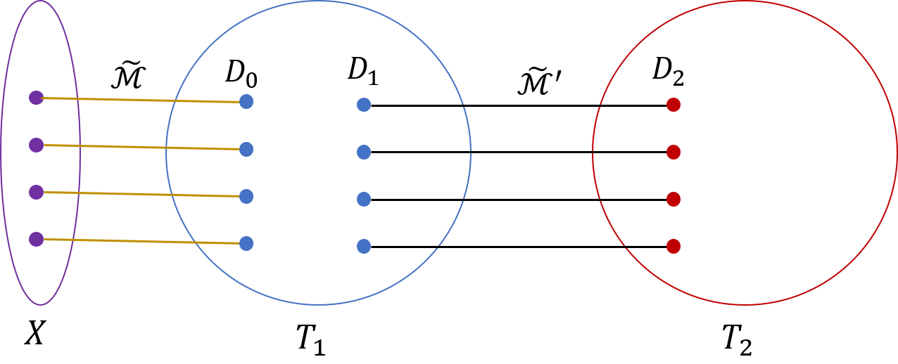 Figure 8
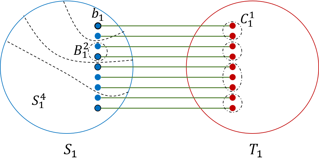 Figure 9
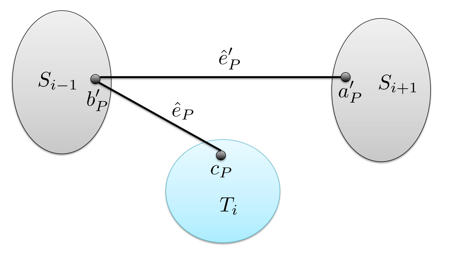 Figure 10
 Figure 11
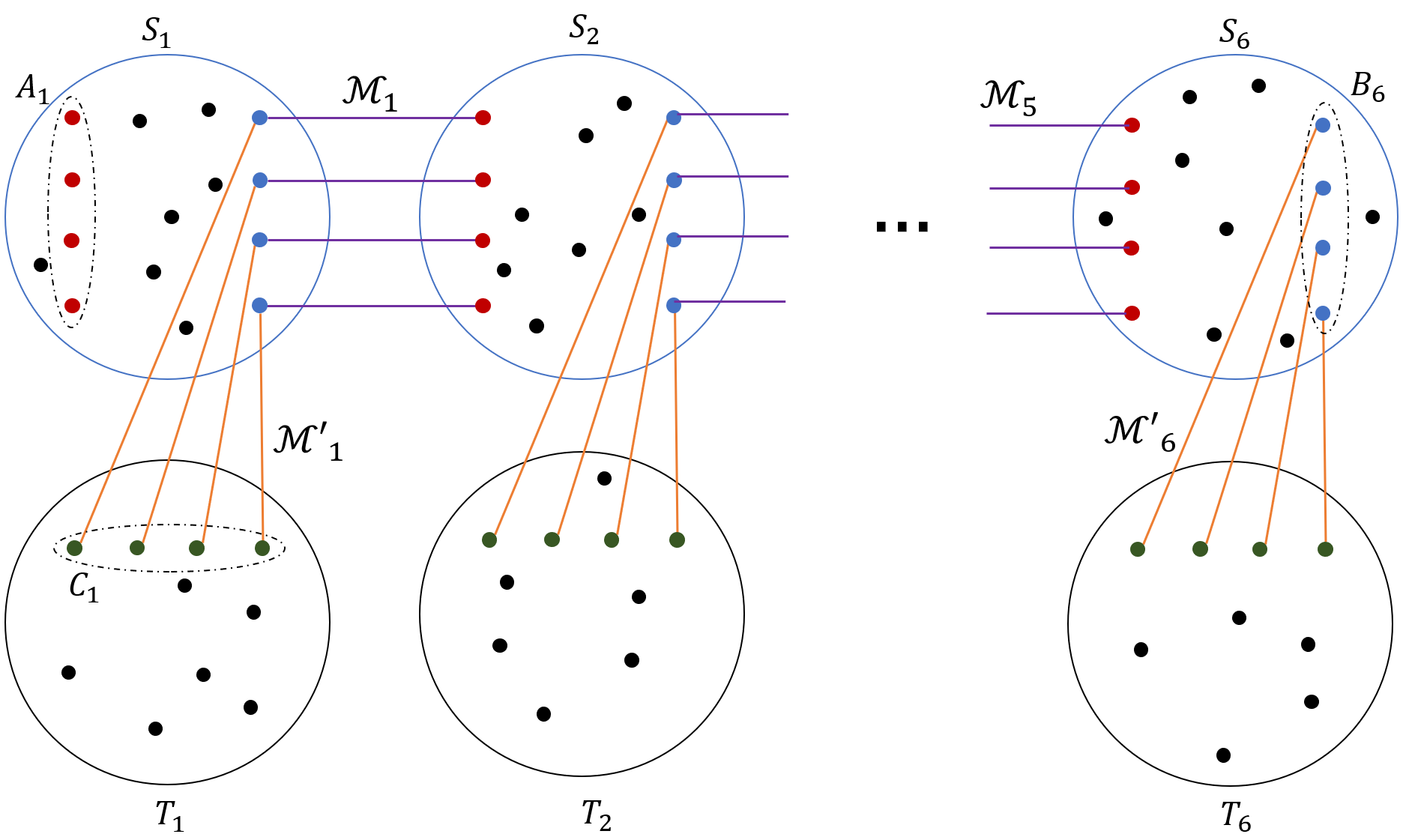 Figure 12
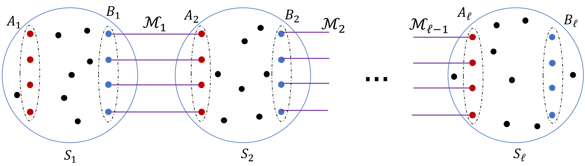 Figure 13
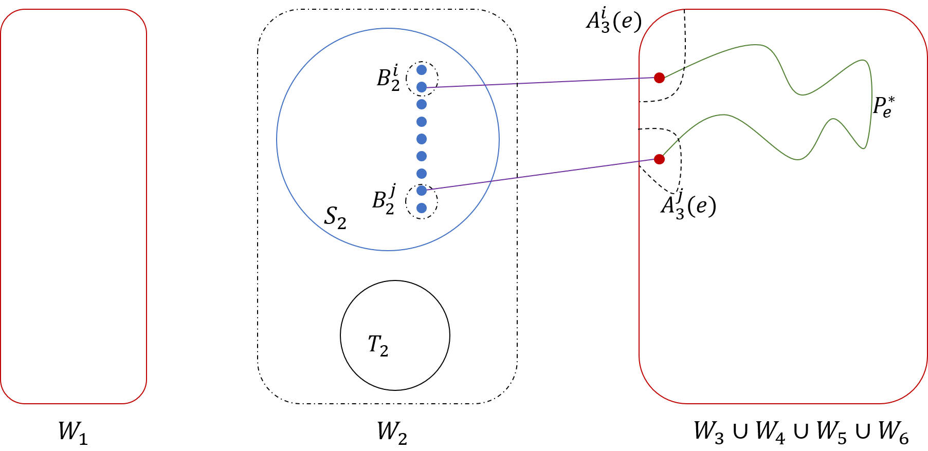 Figure 14
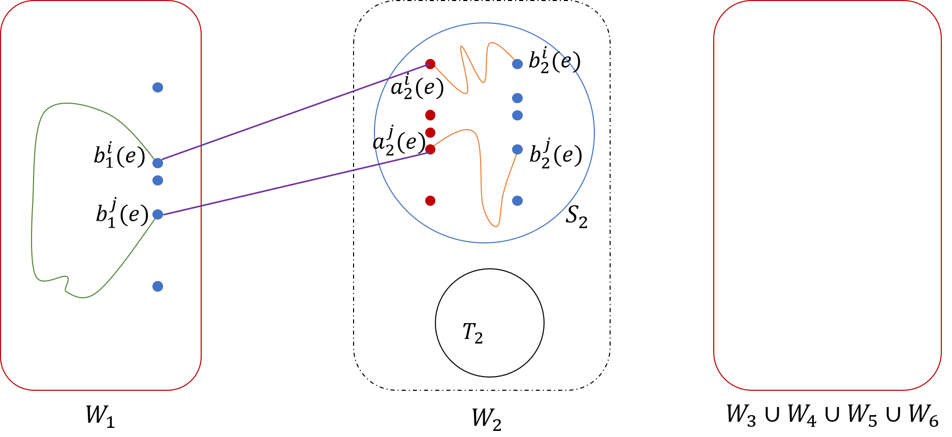 Figure 15
 Figure 16
 Figure 17
Peer Reviews
No public reviews on file for this paper yet. If you reviewed it on a platform where reviews are public (OpenReview, ICLR, NeurIPS, ICML), you can paste yours below so the community can read it here.
Videos
No videos yet. Explain this paper in a talk, walkthrough, or lecture? Add one.
Large Minors in Expanders
Julia Chuzhoy Toyota Technological Institute at Chicago. Email: [email protected]. Part of the work was done while the author was a Weston visiting professor in the Department of Computer Science and Applied Mathematics, Weizmann Institute. Supported in part by NSF grant CCF-1616584.
Rachit Nimavat Toyota Technological Institute at Chicago. Email: [email protected]. Supported in part by NSF grant CCF-1616584.
In this paper we study expander graphs and their minors. Specifically, we attempt to answer the following question: what is the largest function , such that every -vertex -expander with maximum vertex degree at most contains every graph with at most edges and vertices as a minor? Our main result is that there is some universal constant , such that . This bound achieves a tight dependence on : it is well known that there are bounded-degree -vertex expanders, that do not contain any grid with vertices and edges as a minor. The best previous result showed that , where depends on both and . Additionally, we provide a randomized algorithm, that, given an -vertex -expander with maximum vertex degree at most , and another graph containing at most vertices and edges, with high probability finds a model of in , in time . We also show a simple randomized algorithm with running time , that obtains a similar result with slightly weaker dependence on but a better dependence on and , namely: if is an -vertex -expander with maximum vertex degree at most , and contains at most edges and vertices, where is an absolute constant, then our algorithm with high probability finds a model of in .
We note that similar but stronger results were independently obtained by Krivelevich and Nenadov: they show that , and provide an efficient algorithm, that, given an -vertex -expander of maximum vertex degree at most , and a graph with vertices and edges, finds a model of in .
Finally, we observe that expanders are the ‘most minor-rich’ family of graphs in the following sense: for every -vertex and -edge graph , there exists a graph with vertices and edges, such that is not a minor of .
1 Introduction
In this paper we study large minors in expander graphs. A graph is an -expander, if, for every partition of its vertices into non-empty subsets, the number of edges connecting vertices of to vertices of is at least . We say that is an expander, if it is an -expander for some constant , that is independent of the graph size. A graph is a minor of a given graph , if one can obtain a graph isomorphic to from , via a sequence of edge- and vertex-deletions and edge-contractions.
Bounded-degree expanders are graphs that are simultaneously extremely well connected, while being sparse. Expanders are ubiquitous in discrete mathematics, theoretical computer science and beyond, arising in a wide variety of fields ranging from computational complexity to designing robust computer networks (see [HLW06] for a survey on expanders and their applications). In this paper we study an extremal problem about expanders: what if the largest function , such that every -vertex -expander with maximum vertex degree at most contains every graph with at most vertices and edges as a minor?
Our main result is that there is a constant , such that . As we discuss below, this result achieves an optimal dependence on . We also provide a randomized algorithm that, given an -vertex -expander with maximum vertex degree at most , and another graph containing at most edges and vertices, with high probability finds a model of in , in time . Additionally, we show a simple randomized algorithm with running time , that achieves a bound that has a slightly worse dependence on but a better dependence on and : if is an -vertex -expander with maximum vertex degree at most , and is any graph with at most edges and vertices, for some universal constant , the algorithm finds a model of in with high probability.
Independently from our work, Krivelevich and Nenadov (see Theorem 8.1 in [Kri18a]) provide an elegant proof of a similar but stronger result: namely, they show that , and provide an efficient algorithm, that, given an -vertex -expander of maximum vertex degree at most , and a graph with vertices and edges, finds a model of in .
One of our main motivations for studying this question is the Excluded Grid Theorem of Robertson and Seymour. This is a fundamental result in graph theory, that was proved by Robertson and Seymour [RS86] as part of their Graph Minors series. The theorem states that there is a function , such that for every integer , every graph of treewidth at least contains the -grid as a minor. The theorem has found many applications in graph theory and algorithms, including routing problems [RS95], fixed-parameter tractability [DH08, DH07], and Erdős-Pósa-type results [RS86, Car88, Ree97, FST11]. For an integer , let be the smallest value, such that every graph of treewidth at least contains the -grid as a minor. An important open question is establishing tight bounds on the function . Besides being a fundamental graph-theoretic question in its own right, improved upper bounds on directly affect the running times of numerous algorithms that rely on the theorem, as well as parameters in various graph-theoretic results, such as, for example, Erdős-Pósa-type results.
In a series of works [RS86, RST94, KK12, LS15, CC16, Chu15, Chu16a, CT], it was shown that holds. The best currently known negative result, due to Robertson et al. [RST94] is that . This is shown by employing a family bounded-degree expander graphs of large girth. Specifically, consider an -vertex expander whose maximum vertex degree is bounded by a constant independent of , and whose girth is . It is not hard to show that the treewidth of is . Assume now that contains the -grid as a minor, for some value . Such a grid contains disjoint cycles, each of which must consume vertices of , and so . This simple argument is the best negative result that is currently known for the Excluded Grid Theorem. In fact, Robertson and Seymour conjecture that this bound is tight, that is, must hold. A natural question therefore is whether this analysis is tight, and in particular, whether every -vertex bounded-degree expander must contain a -grid as a minor, for . In this paper we answer this question in the affirmative, and moreover, we show that every graph with at most vertices and edges is a minor of such an expander.
The problem of finding large minors in bounded-degree expanders was first considered by Kleinberg and Rubinfield [KR96]. Building on the random walk-based techniques of Broder et al. [BFU94], they showed that every expander on vertices contains every graph with vertices and edges as a minor. The exponent depends on the expansion and the maximum degree of the expander; we estimate it to be at least . They also show an efficient algorithm for finding a model of such a graph in .
Another related direction of research is the existence of large clique minors in graphs. The study of the size of the largest clique minor in a graph is motivated by Hadwiger’s conjecture, which states that, if the chromatic number of a graph is at least , then it contains a clique with vertices as a minor. One well-known result in this area, due to Kawarbayashi and Reed [KR10], shows that every -expander with vertices and maximum vertex-degree bounded by contains a clique with vertices as a minor. Recently, Krivelevich and Nenadov [KN18] improved the dependence on the expansion and the maximum vertex degree under a somewhat stronger definition of expansion. We note that both these bounds have tight dependence on , since contains only edges. Our results imply a weaker bound of on the size of the clique minor, for some absolute constant .
The existence of large clique minors was also studied in the context of random graphs. Recall that is a random graph on vertices, whose edges are added independently with probability each. Bollobás, Catlin and Erdős [BCE80] showed that Hadwiger’s conjecture is true for almost all graphs for every constant . Fountoulakis et al. [FKO09] later showed that for every , there is a constant such that the following is true: if is the probability that the graph does not contain a clique minor on vertices, then . Using a theorem from [Kri18b], our results imply a slightly weaker bound of on the clique minor size.
Our Results and Techniques.
All graphs that we consider are finite; they do not have loops or parallel edges. Given a graph , we define its size to be . Our main result is summarized in the following theorem:
Theorem 1.1**.**
*There is a constant , such that for all and , if is an -vertex -expander with maximum vertex degree at most , and is any graph of size at most , then is a minor of . Moreover, there is a randomized algorithm, whose running time is , that, given and as above, with high probability, finds a model of in . *
As discussed above, the theorem implies that we cannot get stronger negative results for the Excluded Grid Theorem using bounded-degree -expanders, where is independent of the graph size. But this leaves open the possibility of obtaining stronger negative results when is a function of , such as, for example, , or for some small constant . Our next result provides a simpler algorithm, with better running time and a better dependence on and , at the cost of slightly weaker dependence on in the minor size.
Theorem 1.2**.**
*There is a constant and a randomized algorithm, that, given an -vertex -expander with maximum vertex degree at most , where , and another graph of size at most , with high probability computes a model of in , in time . *
The following corollary easily follows from Theorem 1.1 and a result of [Kri18b].
Corollary 1.3**.**
*For every , there is a constant depending only on , such that a random graph with high probability contains every graph of size at most as a minor. *
As mentioned earlier, similar but somewhat stronger results were obtained independently by Krivelevich and Nenadov (see Theorem 8.1 in [Kri18a]).
As a final comment, we show in Appendix B that expanders are the ‘most minor-rich’ family of graphs:
Observation 1.4**.**
*For every graph of size , there is a graph of size at most such that does not contain as a minor. *
We now turn to describe our techniques, starting with the simpler result: Theorem 1.2. Given an -vertex -expander with maximum vertex degree at most , we compute a partition of into two disjoint subgraphs, and , such that is a connected graph; is an -expander for a somewhat weaker parameter , and a large matching connecting vertices of to vertices of . We refer to the edges of , and to their endpoints, as terminals. Assume now that we are given a graph , containing at most vertices and edges. We can assume w.l.o.g. that the maximum vertex degree in is at most , as we can compute a graph of size at most twice the size of , such that the maximum vertex degree of is at most , and is a minor of . Using the transitivity of the minor relation, it is now sufficient to show that is a minor of . Therefore, we assume that the maximum vertex degree in is at most , and we denote . Using the standard grouping technique, we partition the graph into connected subgraphs , each of which contains at least terminals. Assume that . We map the vertex of to the graph . Let be the set of edges of incident to the vertices of . Every edge is embedded into a path in the expander , that connects some edge of to some edge of . The paths are found using standard techniques: we use the classical result of Leighton and Rao [LR99] to show that for every edge of , there is a large set of paths in , connecting edges of to edges of , such that all resulting paths in are short, and cause a small vertex-congestion in . We then use the constructive proof of the Lovasz Local Lemma by Moser and Tardos [MT10] to select a single path from each such set , so that the resulting paths are disjoint in their vertices.
The proof of Theorem 1.1 is somewhat more complex. As before, we assume w.l.o.g. that maximum vertex degree in the graph is at most . We define a new combinatorial object called a Path-of-Expanders System (see Figure 1). At a high level, a Path-of-Expanders System of width and expansion consists of 12 graphs: graphs that are -expanders, and graphs that are connected graphs. For each , we are also given a matching of cardinality connecting vertices of to vertices of ; the endpoints of the edges of in and are denoted by and , respectively. For each , we are given a matching connecting every vertex of to some vertex of ; the endpoints of the edges of that lie in are denoted by . We show that an -vertex -expander with maximum vertex degree at most must contain a Path-of-Expanders System of width and expansion for some constants and , and provide an algorithm with running time to compute it. Next, we split the Path-of-Expanders System into three parts. The first part is the union of the graphs and the matching . We view the vertices of as terminals, and we use the graph and the matching in order to partition them into large enough groups, and to define a connected sub-graph of spanning each such group, like in the proof of Theorem 1.2. We ensure that the number of groups is equal to the number of vertices in the graph that we are trying to embed into . Every vertex of is then embedded into a separate group, together with the corresponding connected sub-graph of spanning the group.
We use the graphs in order to route all but a small fraction of the edges of . The algorithm in this part is inspired by the algorithm of Frieze [Fri01] for routing a large set of demand pairs in an expander graph via edge-disjoint paths. Lastly, the remaining edges of are routed in graph , using essentially the same algorithm as the one in the proof of Theorem 1.2.
Organization.
We start with Preliminaries in Section 2. The proof of Theorem 1.1 is provided in Section 3, with some of the technical details deferred to Sections 4 and 5. Section 6 contains an algorithm for constructing a Path-of-Expanders System. The proof of Theorem 1.2 appears in Section 7, and the proofs of Corollary 1.3 and Observation 1.4 appear in Sections A and B of the Appendix, respectively.
2 Preliminaries
Throughout the paper, for an integer , we denote . All logarithms in the paper are to the base of .
All graphs that we consider are finite; they do not have loops or parallel edges.
We will use the following simple observation, whose proof is deferred to the Appendix.
Observation 2.1**.**
*There is an efficient algorithm, that, given a set of non-negative integers, with , and for all , computes a partition of , such that and . *
Given a graph and a subset of its vertices, we denote by the set of all edges that have exactly one endpoint in , and by the set of all edges with both endpoints in . For readability, we write instead of . Given a pair of disjoint subsets of vertices, we denote by the set of all the edges with one endpoint in and another in . We will omit the subscript when the underlying graph is clear from context. For a subset of vertices of , we denote by the subgraph of induced by .
Given a path in a graph , we denote by and the sets of all its vertices and edges, respectively. Given a path and a set of vertices of , we say that is disjoint from iff . We say that is internally disjoint from iff every vertex of is an endpoint of .
Similarly, suppose we are given two paths in a graph . We say that the two paths are disjoint iff , and we say that they are internally disjoint iff all vertices in serve as endpoints of both these paths.
Let be any set of paths in a graph . We say that is a set of disjoint paths iff every pair of distinct paths are disjoint. We say that is a set of internally disjoint paths iff every pair of distinct paths are internally disjoint. We denote by the set of all vertices participating in the paths of . Given a pair of subsets of vertices of (that are not necessarily disjoint), we say that a path connects to iff one of its endpoints is in and the other endpoint is in . We use a shorthand to indicate that is a collection of disjoint paths, where each path connects to . Notice that each path in must originate at a distinct vertex of and terminate at a distinct vertex of .
Finally, assume that we are given a (partial) matching over the vertices of , and a set of paths. We say that routes iff for every pair of vertices , there is a path , whose endpoints are and .
Sparsest Cut and Expansion.
A cut in is a bipartition of its vertices, that is, , and . The sparsity of the cut is . The expansion of a graph , denoted by , is the minimum sparsity of any cut in .
Definition 1**.**
*Given a parameter , we say that a graph is an -expander iff . Equivalently, for every subset of at most vertices of , . *
The following theorem follows from the standard Cheeger’s inequality, that shows that for any graph , whose maximum vertex degree is bounded by , , where is the second smallest eigenvalue of the Laplacian of , and from the algorithm of [Fie73] (see also [AM84, Alo86, Alo98]).
Theorem 2.2**.**
*There is an efficient algorithm, that, given an -vertex graph with maximum vertex degree at most , computes a cut in of sparsity . *
Finally, we use the following simple claim several times; the claim allows one to “fix” an expander, after a small number of edges were deleted from it. The proof appears in Appendix.
Claim 2.3**.**
*Let be an -expander, and let be any subset of edges of . Then there is an -expander , with . *
Graph Minors.
Definition 2** (Graph Minors).**
We say that a graph is a minor of a graph iff there is a map , called a model of in , mapping every vertex to a subset of vertices, and mapping every edge to a path in , such that:
- •
For every vertex , is connected;
- •
For every edge , the path connects to ;
- •
For every pair of distinct vertices, ; and
- •
Paths are internally disjoint from each other and they are internally disjoint from the set of vertices.
*For a vertex we sometimes call the embedding of into , and for an edge , we sometimes refer to as the embedding of into . *
Well-Linkedness and Path-of-Sets System.
We use a slight variation of the standard definition of (node)-well-linkedness.
Definition 3** (Well-Linkedness).**
*We say that a set of vertices in a graph is well-linked iff for every pair of disjoint equal-cardinality subsets of , there is a set of paths in , that are internally disjoint from . (Note that the paths in must be disjoint). *
Next, we define a Path-of-Sets system, that was first introduced in [CC16] (a somewhat similar object called grill was introduced by [LS15]), and was used since then in a number of graph theoretic results.
Definition 4** (Path-of-Sets System).**
Given integers a Path-of-Sets System of width and length (see Figure 2) consists of:
- •
a sequence of disjoint connected graphs, that we refer to as clusters;
- •
for each , two disjoint subsets, of vertices each; and
- •
For each , a collection of edges, connecting every vertex of to a distinct vertex of .
We denote the Path-of-Sets System by , where . We also denote by the graph defined by the Path-of-Sets System, that is, .
*We say that a given Path-of-Sets System is a Strong Path-of-Sets System iff all , the vertices of are well-linked in . We say that it is -expanding, iff for all , graph is an -expander. Note that a Strong Path-of-Sets System is not necessarily -expanding and vice versa. *
2.1 Path-of-Expanders System
Path-of-Expanders System is the main new structural object that we use.
Definition 5** (Path-of-Expanders System).**
Given an integer and a parameter , a Path-of-Expanders System of width and expansion (see Figure 1) consists of:
- •
a Strong Path-of-Sets System of width and length ;
- •
a sequence of disjoint connected graphs, such that for each , is disjoint from , and it is an -expander; and
- •
for each , a perfect matching between and some subset of vertices of .
*We denote the Path-of-Expanders System by , where . For convenience, for each , we denote by be the graph obtained from the union of the graphs and , and the matching . *
Similarly to the Path-of-Sets System, we associate with the Path-of-Expanders System a graph , obtained by taking the union of the graphs , and the sets of edges.
We will be interested in three subgraphs of (see Figure 3): (i) Graph , that we denote by ; (ii) Graph ; and (iii) Graph , obtained by taking the union of and the edges of .
Definition 6**.**
*We say that a graph contains a Path-of-Sets System of width and length as a minor iff there is a Path-of-Sets System of width and length , such that its corresponding graph is a minor of . Similarly, we say that a graph contains a Path-of-Expanders System of width and expansion as a minor iff there is a Path-of-Expanders System of width and expansion , such that its corresponding graph is a minor of . *
The following theorem, that we prove in Section 6, shows that an expander must contain a Path-of-Expanders System with suitably chosen parameters, and provides an algorithm to compute its model in the expander.
Theorem 2.4**.**
*There are constants , and an algorithm, that, given an -expander with , whose maximum vertex degree is at most , and , constructs a Path-of-Expanders System of expansion and width , such that the corresponding graph has maximum vertex degree at most and is a minor of . Moreover, the algorithm computes a model of in . The running time of the algorithm is . *
3 Proof of Theorem 1.1
The goal of this section is to prove Theorem 1.1. We prove it by using the following theorem.
Theorem 3.1**.**
*There is constant and a randomized algorithm, that, given a Path-of-Expanders System with expansion and width , such that the maximum vertex degree in is at most and for some , together with a graph of maximum vertex degree at most and , with high probability, in time , finds a model of in . *
Before proving Theorem 3.1, we complete the proof of Theorem 1.1 using it. Let be the given -expander with , and maximum vertex degree at most . Recall that . By letting be a sufficiently large constant, we can assume that is sufficiently large, so that, for example, , where is the constant from Theorem 3.1. Indeed, otherwise, it is enough to show that the graph with vertex is a minor of , which is trivially true. Therefore, we assume from now on that is sufficiently large. From Theorem 2.4, contains as a minor a Path-of-Expanders System of width and expansion , such that the maximum vertex degree in is at most . Using these bounds, we get that:
[TABLE]
for . Therefore, if is a graph with maximum vertex degree at most , and , then, from Theorem 3.1, contains as a minor, and from Theorems 2.4 and 3.1, its model in can be computed with high probability by a randomized algorithm, in time .
Consider now any graph of size at most . Let and , so . We construct another graph , whose maximum vertex degree is at most and , such that is a minor of . Since must be a minor of , it follows that is a minor of . In order to construct graph from , we consider every vertex of degree in turn, and replace it with a cycle on vertices, such that every edge incident to in is incident to a distinct vertex of . It is easy to verify that the resulting graph has maximum vertex degree at most , that is a minor of , and that , completing the proof of Theorem 1.1. Notice that this proof is constructive, that is, there is a randomized algorithm that constructs a model of in in time . The remainder of this section is dedicated to proving Theorem 3.1, with some details deferred to subsequent sections.
3.1 Large Minors in Path-of-Expanders System
This subsection is devoted to the proof Theorem 3.1. We assume that we are given a Path-of-Expanders System of width and expansion , whose corresponding graph contains at most vertices, where for some large enough constant , and its maximum vertex degree is bounded by . In order to simplify the notation, we denote by . We also use the following parameter: .
We are also given a graph of maximum degree , with .
Our goal is to find a model of in . Our algorithm consists of three steps. In the first step, we associate with each vertex , a subset of vertices of , such that is a connected graph. This defines the embeddings of the vertices of into for the model of that we are computing. In the second step, we embed all but a small fraction of the edges of into , and in the last step, we embed the remaining edges of into . We now describe each step in detail.
Step 1: Embedding the Vertices of .
In this step we compute an embedding of every vertex of into a connected subgraph of . Recall that graph is the union of the graphs and , and the matching , connecting the vertices of to the vertices of , where . We use the following simple observation, that was used extensively in the literature (often under the name of “grouping technique”) (see e.g. [CKS05, RZ10, And10, Chu16b]). The proof is deferred to Section D of the Appendix.
Observation 3.2**.**
There is an efficient algorithm that, given a connected graph with maximum vertex degree at most , an integer , and a subset of vertices of with , computes a collection of mutually disjoint subsets of , such that:
- •
For each , the induced graph is connected; and
- •
For each , .
We apply the above observation to the graph , together with vertex set and parameter . Let be the resulting collection of subsets of vertices of . Recall that for each set , . Since , we can choose distinct sets . We also denote . Finally, for each , we let be the subset of edges that have an endpoint in , and we let be the subset of vertices of that serve as endpoints of the edges in . Since , for all . We are now ready to define the embeddings of the vertices of into . For each , we let . Notice that for all , is a connected graph, and for all , . In the remaining steps, we focus on embedding the edges of into , such that the resulting paths are internally disjoint from .
Step 2: Routing in .
Consider some vertex , its corresponding graph , and the set of vertices that lie in ; recall that . Recall that the maximum vertex degree in is at most . For every edge , we select an arbitrary subset of vertices, so that all resulting sets are mutually disjoint.
Recall that graph contains a perfect matching between the vertices of and the vertices of . We let be the subset of edges whose endpoints lie in , and denote by the set of endpoints of the edges of that lie in . For every edge , we let be the set of vertices that are connected to the vertices of with an edge of . Clearly, all resulting vertex sets are mutually disjoint. Let , and notice that
[TABLE]
The following lemma, whose proof is deferred to Section 4, allows us to embed a large number of edges of in .
Lemma 3.3**.**
*There is an efficient algorithm, that, given a Path-of-Expanders System of expansion and width , where and is an integral multiple of , whose corresponding graph contains at most vertices and has maximum vertex degree at most , together with a subset of at most vertices, and a collection of mutually disjoint subsets of of cardinality each, where , returns a partition of , and a set of disjoint paths in , such that for each , path connects to , and . *
We obtain the following immediate corollary of the lemma.
Corollary 3.4**.**
*There is an efficient algorithm to compute a partition of the set of edges of , and for each edge , a path in graph , connecting a vertex of to a vertex of , such that all paths in set are disjoint, and . *
Proof.
By appropriately ordering the collection of vertex subsets, and applying Lemma 3.3 to the resulting sequence of subsets of , we obtain a set of edges of , and for each edge , a path , connecting a vertex of to a vertex of in graph , such that all paths in set are disjoint. Let . From Lemma 3.3, .
For each edge , we extend the path to include the two edges of incident to its endpoints, so that now connects a vertex of to a vertex of . Path becomes the embedding of in the model of that we are constructing. For convenience, the resulting set of paths is still denoted by . The paths in remain disjoint from each other; they are internally disjoint from , and completely disjoint from (see Figure 5).
Step 3: Routing in .
In this step we complete the construction of a minor of in , by embedding the edges of . The main tool that we use is the following lemma, whose proof is deferred to Section 5.
Lemma 3.5**.**
There is a universal constant , and an efficient algorithm that, given a Path-of-Expanders System of expansion and width , such that the corresponding graph contains at most vertices and has maximum vertex degree at most , computes a subset of at least vertices, such that the following holds. There is an efficient randomized algorithm, that given any matching over the vertices of , with high probability returns a set of disjoint paths in , routing .
We now conclude the last step using the above lemma. Let be the subset of at least vertices, computed by algorithm from Lemma 3.5. Let be the set of all the vertices connected to the vertices of by the edges of the matching . Observe that , since:
[TABLE]
since we have assumed that is sufficiently large. We let be an arbitrary subset of vertices of .
Recall that every vertex , and edge , we have defined a subset of vertices. We select an arbitrary representative vertex , and we let be the resulting set of representative vertices, so that .
Since are well-linked in , there is a set of disjoint paths in , connecting every vertex of to some vertex of , such that the paths in are internally disjoint from . For each vertex , let be the corresponding endpoint of the path of that originates at (see Figure 6). Let be the vertex of that is connected to with an edge from . We can now naturally define a matching over the vertices of , where for every edge , we add the pair of vertices to the matching. From Lemma 3.5, with high probability we obtain a collection of disjoint paths in , such that, for every edge , the corresponding path connects to . We extend this path to connect the vertex to the vertex , by using the edges of that are incident to to , and the paths of that are incident to to . Notice that the resulting extended paths are internally disjoint from , and are completely disjoint from . We now embed each edge into the path , that is, we set . This completes the construction of the model of in , except for the proofs of Lemmas 3.3 and 3.5, that are provided in Sections 4 and 5, respectively.
4 Routing in
This section is dedicated to the proof of Lemma 3.3. We define a new combinatorial object, called a Duo-of-Expanders System.
Definition 7**.**
A Duo-of-Expanders System of width , expansion (see Figure 7) consists of:
- •
two disjoint graphs , each of which is an -expander;
- •
a set of vertices that are disjoint from , and three subsets and of vertices each, where all three subsets are disjoint; and
- •
a complete matching between the vertices of and the vertices of , and a complete matching between the vertices of and the vertices of , so .
*We denote the Duo-of-Expanders System by . The set of vertices is called the backbone of . Let be the graph corresponding to the Duo-of-Expanders System , so is the union of graphs , the set of vertices, and the set of edges. *
Similarly to Path-of-Expanders System, given a graph , we say that it contains a Duo-of-Expanders System as a minor iff is a minor of .
The following lemma is central to the proof of Lemma 3.3.
Lemma 4.1**.**
*There is an efficient algorithm that, given a Duo-of-Expanders System of width and expansion , for some , such that the corresponding graph contains at most vertices and has maximum vertex degree at most , together with a collection of mutually disjoint subsets of the backbone of cardinality each, where , returns a partition of , and for each , a path connecting a vertex of to a vertex of in , such that the paths in set are disjoint, and . *
We defer the proof of Lemma 4.1 to Section 4.1, after we complete the proof of Lemma 3.3 using it. Recall that we are given a Path-of-Expanders System , together with its corresponding graph . Recall that we are also given a subset of at most vertices, and a partition of into disjoint subsets , of cardinality each, where . For each , we arbitrarily partition into two subsets, , of cardinality each (note that is an even integer). Let and let . Note that . We add arbitrary vertices of to and , until each of them contains vertices (recall that is an integer), while keeping them disjoint. The vertices of are then arbitrarily partitioned into two subsets, and , of cardinality each.
Next, we show that graph contains two disjoint Duo-of-Expanders Systems as minors. We will then use Lemma 4.1 in each of the two Duo-of-Expanders Systems in turn in order to obtain the desired routing.
Claim 4.2**.**
*There is an efficient algorithm to compute two disjoint subgraphs, and of , and for each , to compute a model of a Duo-of-Expanders System of width and expansion in , such that the corresponding graph has maximum vertex degree at most , and for every vertex , there is a distinct vertex in the backbone , such that . *
Proof of Claim 4.2. From the definition of the Path-of-Expanders System, for , the set of vertices is well-linked in . Therefore, there is a set of node-disjoint paths in , connecting to . By concatenating the path sets , and the edge sets , we obtain a collection of node-disjoint paths in , connecting to . We partition into two subsets: set contains all paths originating at the vertices of , and set contains all paths originating at the vertices of .
We are now ready to define the two graphs and . Graph is obtained from the union of the expanders and , the paths of , and the edges of that have an endpoint lying on the paths of . Graph is defined similarly by using , the paths of , and the edges of that have an endpoint lying on the paths of . It is immediate to verify that the graphs and are disjoint.
It now remains to show that each of the resulting graphs contains a Duo-of-Expanders System as a minor, with the required properties. We show this for ; the proof for is symmetric. Our first step is to contract every path of into a single vertex. For each such path , let be the first vertex of . We denote the new vertex obtained by contracting by . We let the backbone of the new Duo-of-Expanders System be , so . We map every vertex to the corresponding vertex in the model of that we are constructing in ; that is, we set . We also map the two expanders of to and , respectively, by setting and .
Consider some vertex and the path originating from . Let be the unique vertex of that belongs to , and let be the unique vertex of that belongs to , in the original Path-of-Expanders System . Recall that there is an edge of , connecting to some vertex , and there is an edge of , connecting to some vertex . Therefore, there are edges and in the new contracted graph.
We set , and we let . We also set , and . Observe that all three sets of vertices are disjoint, and they contain vertices each. It now remains to define the set of edges, that connect vertices of and . In order to do so, for every vertex , we merge the two edges and into a single edge, by contracting one of these two edges. The resulting edge is added to . It is easy to see that we have obtained a Duo-of-Expanders System , whose width is and expansion . It is easy to verify that the maximum vertex degree in the corresponding graph is bounded by . Notice that for every vertex , there is a distinct vertex , such that .
We apply Lemma 4.1 to , together with vertex sets , each of which now contains vertices obtaining a partition of , together with a set of disjoint paths in , such that for all path connects a vertex of to a vertex of , and . Since is a minor of , it is immediate to obtain a collection of disjoint paths in , such that for all path connects a vertex of to a vertex of .
If , then we terminate the algorithm, and return the set of paths, together with the partition of . Next, we denote , and we assume that .
We apply Lemma 4.1 to , together with vertex sets , that are appropriately ordered. We then obtain a partition of , and a set of disjoint paths in , such that for each path connects a vertex of to a vertex of , and . As before, since is a minor of , it is immediate to obtain a collection of disjoint paths in , such that for all path connects a vertex of to a vertex of .
We return the partition of , together with the set of paths. Since the graphs and are disjoint, all paths in are disjoint. It now only remains to show that .
Recall that the set of at most vertices is partitioned into subsets of cardinality each. Therefore:
[TABLE]
Therefore, , as required.
4.1 Routing in Duo-of-Expanders — Proof of Lemma 4.1
The goal of this section is to prove Lemma 4.1. The proof is inspired by the algorithm of Frieze [Fri01] for routing a large set of demand pairs in an expander graph via edge-disjoint paths. Recall that we are given a Duo-of-Expanders System of width and expansion , for some , such that the maximum vertex degree in the corresponding graph is at most , and . We are also given mutually disjoint subsets of the backbone , of cardinality each, where . In particular, since , we get that , and so . Therefore, we obtain the following bounds on that we will use throughout the proof:
[TABLE]
For convenience, we will denote by for the rest of this subsection.
We will iteratively construct the set of disjoint paths in , where for each path , there is some index , such that connects to . Whenever a path is added to , we delete all vertices of from . Throughout the algorithm, we say that an index is settled iff there is a path connecting to , and otherwise we say that it is not settled. We use a parameter . We say that a path in is permissible iff contains at most nodes of and at most nodes of .
The Algorithm.
Start with . While there is an index and a permissible path in the current graph such that:
- •
is not settled;
- •
connects to ; and
- •
is internally disjoint from :
add to and delete all vertices of from .
In order to complete the proof of Lemma 4.1, it is enough to show that, when the algorithm terminates, at most indices are not settled. Assume for contradiction that this is not true. Let be the path set obtained at the end of the algorithm, and let be the set of vertices participating in the paths of . We further partition into three subsets: ; ; and . Note that, since , we are guaranteed that ; , and, since we have assumed that , and all paths in are internally disjoint from , we get that .
We now proceed as follows. First, we show that and both contain very large -expanders. We also show that there is a large number of edges in that connect these two expanders. This will be used to show that there must still be a permissible path , connecting two sets and for some index that is not settled yet, leading to a contradiction. We start with the following claim that allows us to find large expanders in and .
Claim 4.3**.**
*Let be an -expander with maximum vertex degree at most , and let be any subset of vertices of . Then there is an -expander , with . *
The proof of Claim 4.3 follows immediately from Claim 2.3, by letting be the set of all edges incident to the vertices of . The following corollary follows immediately from Claim 4.3
Corollary 4.4**.**
*There is a subgraph that is an -expander, and . Similarly, there is a subgraph that is an -expander, and . *
Let and let . We refer to the vertices of and as the vertices that were discarded from and , respectively. The vertices that belong to and are called surviving vertices. It is easy to verify that . Indeed, observe that . Since, from Equation (1), , we get that altogether:
[TABLE]
since .
Recall that the Duo-of-Expanders contains a matching between the set of vertices and the set of vertices. Next, we show that there are large subsets and of surviving vertices, such that a subset of defines a complete matching between them.
Observation 4.5**.**
*There are two sets and containing at least vertices each, and a subset of edges, such that is a complete matching between and . *
Proof.
Let . Since , . Let be the set of edges whose endpoints lie in , and let be the set of vertices that serve as endpoints for the edges in , so . Finally, let , so . We let be the set of all edges incident to the vertices of , and we let be the set of endpoints of these edges.
Our second main tool is the following claim, that shows that for any pair of large enough sets of vertices in an expander, there is a short path connecting them. The proof uses standard methods and is deferred to Appendix.
Claim 4.6**.**
*Let be an -expander for some , such that , and the maximum vertex degree in is at most . Let be two vertex subsets, with and . Then there is a path in , connecting a vertex of to a vertex of , whose length is at most . In particular, for every pair of vertices in , there is a path of length at most connecting to in . *
Let be the set of indices that are not settled yet. From our assumption, . For every index , consider the corresponding sets of vertices of , and let be the sets of vertices of , that are connected to and via the matching . Let and let be the subsets of surviving vertices in and respectively. We say that index is bad iff or ; otherwise we say that it is a good index. Recall that . Therefore, the total number of bad indices is at most:
[TABLE]
since .
Let be the set of all good indices, so . We say that an index is happy iff there is a path in , of length at most , connecting a vertex of to a vertex of , and there is a path in , of length at most , connecting a vertex of to a vertex of . The following claim will finish the proof of Lemma 3.3.
Claim 4.7**.**
*At least one index of is happy. *
Assume first that the claim is correct. Consider the paths and in , given by Claim 4.7, and assume that path connects a vertex to a vertex . Let be the vertex connected to by an edge of , that we denote by . Similarly, assume that path connects a vertex to a vertex . Let be the vertex connected to by an edge of , that we denote by . From Claim 4.6, there is a path in , of length at most , connecting to . By combining , together with the edges of incident to and , we obtain an admissible path, connecting a vertex of to a vertex of , a contradiction. It now remains to prove Claim 4.7.
Proof of 4.7. We say that a vertex of is happy iff there is a path in , of length at most , connecting to a vertex of . Assume for contradiction that the claim is false. Then for each good index , either all vertices of are unhappy, or all vertices of are unhappy. Let be the set of all unhappy vertices. Since , and , we get that:
[TABLE]
Let , so . From Claim 4.6, there is a path in , connecting a vertex of to a vertex of , of length at most: , since .
5 Routing in
The goal of this section is to prove Lemma 3.5. We use the following lemma, whose proof uses standard techniques and is deferred to Section F of Appendix.
Lemma 5.1**.**
There is a universal constant , and an efficient randomized algorithm, that, given graph with , such that the maximum vertex degree in is at most and a parameter , together with a collection of mutually disjoint subsets of of cardinality each, computes one of the following:
- •
either a collection of paths in , where for each , path connects a vertex of to a vertex of , and with high probability the paths in are disjoint; or
- •
a cut in of sparsity less than .
Consider the subgraph of ; recall that it consists of two graphs, and , where is a connected graph and is an -expander. Recall that contains a set of vertices; contains a set of vertices, and is a perfect matching between these two sets.
We let , where is the constant from Lemma 5.1, and we let . Observe that . We use Observation 3.2 to compute connected subgraphs of , each of which contains at least vertices of . For , we denote . We also let be the set of edges incident to the vertices of in , and we let be the set of the endpoints of the edges of that lie in . Observe that for all , . For each , we select an arbitrary vertex , and we let , so that , as required.
Assume now that we are given an arbitrary matching over the vertices of . By appropriately re-indexing the sets , we can assume w.l.o.g. that . Since is an -expander, the algorithm of Lemma 5.1 computes a collection of paths in , where for each , path connects some vertex to some vertex , and with high probability the paths in are disjoint.
Consider now some index . We let be the unique edge of the matching incident to , and we let be the other endpoint of this edge. Since graph is connected, and it contains both and , we can find a path in , connecting to . For each , let be the path obtained by concatenating , and let . It is immediate to verify that, if the paths in are disjoint from each other, then so are the paths in , since all graphs in are disjoint from each other and from . Moreover, for each , path connects to , as required.
6 Constructing a Path-of-Expanders System
The goal of this section is to prove Theorem 2.4. The proof consists of three parts. In the first part, we construct an -expanding Path-of-Sets System of length in , for some . In the second part, we transform it into a Strong Path-of-Sets System of the same length. In the third and the final part, we turn the Strong Path-of-Sets System into a Path-of-Expanders System.
6.1 Part 1: Constructing an Expanding Path-of-Sets System
The main technical result of this section is the following theorem.
Theorem 6.1**.**
*There is a constant , and a deterministic algorithm, that, given an -vertex -expander with maximum vertex degree at most , where , computes, in time a partition of , such that , and each graph is an -expander, for . *
The main tool that we use in the proof of the theorem is the following lemma.
Lemma 6.2**.**
*There is a constant , and deterministic algorithm, that, given an -vertex -expander with maximum vertex degree at most , where , computes, in time , a subset of vertices, such that , and is an -expander, for . *
Proof.
Given a graph , we say that a partition of is a balanced cut iff .
Our starting point is the following claim.
Claim 6.3**.**
There is an efficient algorithm that, given an -vertex graph , and a parameter , returns one of the following:
- •
either a subset of vertices, such that and is an -expander;
- •
or a partition of with .
Proof.
We start with an arbitrary balanced cut in with , and perform a number of iterations. In every iteration, we will either establish that is an -expander, or compute the desired partition of , or find a new balanced cut in with . In the first two cases, we terminate the algorithm and return either (in the first case), or the cut (in the second case). In the last case, we replace with , and continue to the next iteration.
We now describe the execution of an iteration. Recall that we are given a balanced cut of with . If , then we return the cut and terminate the algorithm. Therefore, we assume that . We apply the algorithm from Theorem 2.2 to graph , and consider the cut of computed by the algorithm. We then consider two cases. First, if , then from Theorem 2.2, we are guaranteed that is an -expander. We terminate the algorithm and return .
We assume that from now on, and we assume w.l.o.g. that . We consider again two cases. First, if , we define a new cut in , where . We then get that , and moreover, . We return the cut and terminate the algorithm.
The final case is when . In this case, we are guaranteed that . Therefore, if we consider the cut , where and , then is a balanced cut in , and moreover:
[TABLE]
We then replace with the new cut , and continue to the next iteration. It is easy to verify that every iteration can be executed in time . Since the number of the edges in the set decreases in every iteration, the number of iterations is also bounded by .
By combining Claim 6.3 with Observation 2.1, we obtain the following simple corollary.
Corollary 6.4**.**
There is an efficient algorithm that, given an -vertex graph with maximum vertex degree at most , and a parameter , returns one of the following:
- •
either a subset of vertices, such that and is an -expander;
- •
or a balanced partition of with .
Proof.
Throughout the algorithm, we maintain a set of edges of that we remove from the graph, starting with , and a collection of disjoint induced subgraphs of , starting with . The algorithm continues as long as there is some graph , with . In every iteration, we select the unique graph with , and apply Claim 6.3 to it, with the parameter . If the outcome is a subset of vertices, such that , and is an -expander, then we return : it is easy to verify that , so is a valid output. Otherwise, we obtain a partition of with . We add the edges of to , remove from , and add and to instead. If , then our algorithm will never attempt to process the graph again, so we charge the edges of to the vertices of , where every vertex of is charged fewer than units. The algorithm terminates when every graph has (unless it terminates earlier with an expander). Notice that from our charging scheme, at the end of the algorithm, . Moreover, using Observation 2.1, we can partition the final collection of graphs into two subsets, , such that . Letting and , we obtain a balanced partition of . Since , we get that .
We now turn to complete the proof of Lemma 6.2. We denote , and we let . Our goal now is to compute a subset of vertices, with , such that is an -expander, where for some constant . Our algorithm is recursive. Over the course of the algorithm, we will consider smaller and smaller sub-graphs of , containing at least vertices each. For each such subgraph , we define its level as follows. Let . If , then ; otherwise, . Intuitively, is the number of recursive levels that we will use for processing . Notice that, from the definition of , . We use the following claim.
Claim 6.5**.**
There is a deterministic algorithm, that, given a subgraph , such that , and a parameter , returns one of the following:
- •
Either a balanced cut in with ; or
- •
A subset of vertices of , such that , and is an -expander, for .
*The running time of the algorithm is . *
We prove the claim below, after we complete the proof of Lemma 6.2 using it. We apply Claim 6.5 to the input graph and the parameter . Since is an -expander, we cannot obtain a cut in with . Therefore, the outcome of the algorithm is a subset of vertices of , with , such that is a -expander, for , in time . Recall that . Therefore, we get that for some constant , and the running time of the algorithm is . It now remains to prove Claim 6.5.
Proof of Claim 6.5. We denote . We let be a large enough constant. We prove by induction on that the claim is true, with the running time of the algorithm bounded by . The base of the recursion is when , and so . We apply Corollary 6.4 to graph with the parameter . If the outcome of the corollary is a subset of vertices with , such that is an -expander, then we terminate the algorithm and return . Notice that in this case, we are guaranteed that . Otherwise, the algorithm returns a balanced cut in , with . We then return this cut. The running time of the algorithm is .
We now assume that the theorem holds for all graphs with , for some integer , and prove it for a given graph with . Let . The proof is somewhat similar to the proof of Corollary 6.4. Throughout the algorithm, we maintain a balanced cut of , with . Initially, we start with an arbitrary such balanced cut. Notice that . While , we perform iterations (that we call phases for convenience, since each of them consists of a number of iterations). At the end of every phase, we either compute a subset of vertices of , such that , and is an -expander, in which case we terminate the algorithm and return ; or we compute a new balanced cut in , such that . If , then we return this cut; it is easy to verify that . Otherwise, we replace with the new cut , and continue to the next iteration. Since initially , and since decreases by at least in every phase, the number of phases is bounded by . We now proceed to describe a single phase.
An execution of a phase.
We assume that we are given a balanced cut in , with , and . Our goal is to either compute a subset of vertices of such that and is an -expander, or return another balanced cut in , with . Let . Over the course of the algorithm, we will maintain a set of edges that we remove from the graph, starting with , and a collection of subgraphs of (that will contain at most such subgraphs). As each graph is a subgraph of , we are guaranteed that , and so . We start with containing a single graph, the graph . We then iterate, while there is a graph with .
In every iteration, we let be the unique graph with . Notice that , since we have assumed that and so . We apply the algorithm from the induction hypothesis to , with the parameter . If the outcome is a subset of vertices of , such that and is a -expander, for then we terminate the algorithm and return . Notice that, since , and , we get that , so is a -expander. Otherwise, the algorithm returns a balanced cut of , such that . We add the edges of to , remove from , and add and to . The algorithm terminates once for every graph , . Let at the end of the algorithm. Since the cuts that we compute in every iteration are balanced, it is easy to verify that we run the algorithm from the induction hypothesis at most times, and that , since in every iteration the size of the largest graph in decreases by at least factor , and . Denote , and for each , let , and let . Since , there is some index , such that . We define a new balanced cut , by setting and . Since , it is immediate to verify that it is a balanced cut. Moreover, it is immediate to verify that , and so:
[TABLE]
Finally, we bound the running time of the algorithm. The running time is at most plus the time required for the recursive calls to the same procedure. Recall that the number of phases in the algorithm is at most , and every phase requires up to recursive calls. Therefore, the total number of recursive calls is bounded by . Each recursive call is to a graph that has . From the induction hypothesis, the running time of each recursive call is bounded by , and so the total running time of the algorithm is bounded by:
[TABLE]
since .
We are now ready to complete the proof of Theorem 6.1.
Proof of Theorem 6.1. We start with the input -vertex -expander and apply Lemma 6.2 to it, obtaining a subset of vertices, such that is a -expander and . Let . Since the maximum vertex degree in is at most , .
We use the following claim, which is similar to Claim 2.3, except that it provides an efficient algorithm instead of the existential result of Claim 2.3, at the expense of obtaining somewhat weaker parameters. The proof appears in the Appendix.
Claim 6.6**.**
*There is an efficient algorithm, that given an -expander with maximum vertex degree at most and a subset of its edges, computes a subgraph that is an -expander, and . *
We apply Claim 6.6 to graph and the set of edges computed above. Let be the resulting graph, and let . From Claim 6.6, . Since and the set of edges disconnects the vertices of from the rest of the graph, while is an -expander and therefore a connected graph, .
We are now ready to define the final partition of , by letting it be the minimum cut separating the vertices of from the vertices of in : that is, we require that , , and among all such partitions of , we select the one minimizing . The partition can be computed efficiently using standard techniques: we construct a new graph by starting with , contracting all vertices of into a source , contracting all vertices of into a destination , and computing a minimum - cut in the resulting graph. The resulting cut naturally defines the partition of . Let , and denote . From Menger’s theorem, there is a set of edge-disjoint paths in , connecting to . Therefore, there is a set of edge-disjoint paths in , where each path in connects a distinct edge of to a vertex of , and similarly, there is a set of edge-disjoint paths in , where each path in connects a distinct edge of to a vertex of .
We claim that each of the graphs is an -expander, for . We prove this for ; the proof for is similar. Assume for contradiction that is not an -expander. Then there is a cut in , such that . Assume w.l.o.g. that . We now consider two cases.
The first case happens when . In that case, since is an -expander, there are at least edges connecting to , and so , a contradiction. Therefore, we assume now that .
We partition the edges of into two subsets: set contains all edges that lie in , and set contains all remaining edges, so (see Figure 8). Note that from the definition of the cut , . Recall that for every edge , there is a path contained in , connecting to a vertex of , such that all paths in are edge-disjoint. Let be the set of paths originating at the edges of . We further partition into two subsets: set contains all paths that contain an edge of , and contains all remaining paths. Notice that . On the other hand, every path is contained in , and contains a vertex of – the endpoint of . Since we have assumed that , and since the maximum vertex degree in is at most , while the paths in are edge-disjoint, we get that . Altogether, we get that , and , since , as . This contradicts the fact that is an -expander.
Corollary 6.7**.**
*There is an algorithm, that, given, an -vertex -expander with maximum vertex degree at most and an integer , where , computes an -expanding Path-of-Sets system of length and width , together with a subgraph of , where , and is the constant from Theorem 6.1. The running time of the algorithm is . *
We note that we will use the corollary for with , and so the resulting Path-of-Sets System will have expansion , and the running time of the algorithm from Corollary 6.7 is .
Proof.
The proof is by induction on . The base case is when . We choose two arbitrary disjoint subsets of of vertices, and we let . This defines an -expanding Path-of-Sets System of length and width .
We now assume that we are given an integer , and an -expanding Path-of-Sets System of length and width , where . We assume that . We compute an -expanding Path-of-Sets System of length and width . We will denote , and for each , the corresponding vertex sets and in are denoted by and , respectively.
For all , we set . We also let be any subset of vertices, and for , we let be any subset of edges; the endpoints of these edges lying in and are denoted by and respectively. It remains to define , the matchings and (that implicitly define the sets of vertices), and the set of vertices.
We apply Theorem 6.1 to graph , and compute, in time a partition of , such that , and each graph is an -expander, for .
One of the two subsets, say , must contain at least half of the vertices of . We set and . Recall that: . Since graph is an -expander, there are at least edges connecting to . Since maximum vertex degree in is at most , there is a matching , between vertices of and vertices of , with . We claim that . In order to see this, it is enough to prove that . Since , this is equivalent to proving that:
[TABLE]
This is easy to verify from the definition of and the fact that . We let be any subset of containing edges. The endpoints of the edges of lying in and are denoted by and respectively. We let be any subset of vertices of . Finally, we let any subset of vertices of ; the subset of edges whose endpoints lie in ; and the set of endpoints of the edges of lying in . This completes the construction of the Path-of-Sets System . It is immediate to verify that it has length , width , and that . It remains to prove that it is -expanding, or equivalently, that and are -expanders. Recall that Theorem 6.1 guarantees that both these graphs are -expanders, where . It is now enough to verify that , which is immediate to do from the definition of :
[TABLE]
Lastly, the running time of the algorithm is dominated by partitioning , and is bounded by , as required.
We apply Corollary 6.7 to the input graph , with the parameter , obtaining a sub-graph , and an -expanding Path-of-Sets System of length and width , where . The running time of the algorithm is .
6.2 Part 2: From Expanding to Strong Path-of-Sets System
The goal of this subsection is to prove the following theorem:
Theorem 6.8**.**
*There is an efficient algorithm, that, given a parameter , and an -Expanding Path-of-Sets System of width and length , where , such that the corresponding graph has maximum vertex-degree at most , computes a Strong Path-of-Sets System , of width and length , such that the maximum vertex degree in the corresponding graph is at most , and is a minor of . Moreover, the algorithm computes a model of in . *
We use the following simple claim, whose proof is deferred to the Appendix.
Claim 6.9**.**
*There is an efficient algorithm, that, given an -expander , whose maximum vertex degree is at most , where , together with two disjoint subsets of its vertices of cardinality each, computes a collection of disjoint paths, connecting vertices of to vertices of in . *
We will also use the following theorem, whose proof is similar to some arguments that appeared in [CC16], and is deferred to the Appendix.
Theorem 6.10**.**
*There is an efficient algorithm, that, given an -Expanding Path-of-Sets System of width and length , where , and the corresponding graph has maximum vertex degree at most , computes subsets of vertices each, such that is well-linked in . *
We are now ready to complete the proof of Theorem 6.8.
Proof of Theorem 6.8. We construct a Strong Path-of-Sets System of length and width , denoting . For all , the corresponding vertex sets and are denoted by and , respectively.
For all , we let be the -expanding Path-of-Sets System of width and length obtained by using the clusters , , and the matchings and . In order to define the new Path-of-Sets System, for each , we set . We apply Theorem 6.10 to , to obtain subsets , of vertices each, such that are well-linked in .
In order to complete the construction of the Path-of-Sets System , we let be any subset of vertices, and we define similarly. It remains to define, for each , the matching . We will ensure that the endpoints of the resulting matching are contained in and , respectively, ensuring that the resulting Path-of-Sets System is strong.
Consider some index . Recall that we have computed the sets , of vertices. We let be the set of edges incident to the vertices of , and we denote by the set of vertices in that serve as their endpoints. Similarly, we let be the set of edges incident to the vertices of , and we denote by the set of vertices in that serve as their endpoints. From Claim 6.9, there is a set of disjoint paths in , connecting vertices of to vertices of , of cardinality . By extending the paths in to include the edges of incident to them, we obtain a collection of disjoint paths in , connecting vertices of to vertices of . We denote the endpoints of the paths in lying in by , and the endpoints of the paths in lying in by . The paths in naturally define the matching between the vertices of and the vertices of . This concludes the definition of the Path-of-Sets System . It is immediate to verify that it is a strong Path-of-Sets System of length and width , and to obtain a model of in . Note that graph has maximum vertex degree at most .
Recall that in Part 1 of the algorithm, we have obtained a sub-graph , and an -expanding Path-of-Sets System of length and width , where . Applying Theorem 6.8 to , we obtain a Strong Path-of-Sets System of length and width . We have also computed a model of in , and established that the maximum vertex degree in is at most . For convenience, we let be a constant, such that .
6.3 From Strong Path-of-Sets System to Path-of-Expanders System
The goal of this subsection is to prove the following theorem:
Theorem 6.11**.**
*There is an efficient algorithm, that, given a Strong Path-of-Sets System of width and length , such that the corresponding graph has at most vertices and has maximum vertex degree at most , computes a Path-of-Expanders System of width and expansion , whose corresponding graph has maximum vertex degree at most and is a minor of . Moreover, the algorithm computes a model of in . *
Before we prove Theorem 6.11, we complete the proof of Theorem 2.4 using it. Recall that our input is an -expander , for some , with , such that the maximum vertex degree in is at most . Our goal is to provide an algorithm that computes a Path-of-Expanders System of expansion and width , such that the maximum vertex degree in is at most , and to compute a minor of in .
Recall that in Step 2 we have constructed a Strong Path-of-Sets System of length and width , for some constant , such that has maximum vertex degree at most . We have also computed a model of in . Our last step is to apply Theorem 6.11 to . As a result, we obtain a Path-of-Expanders System of width and expansion , whose corresponding graph has maximum vertex degree at most . We also obtain a model of in .
Substituting the value , we get that the width of the Path-of-Expanders System is , and that its expansion is . By appropriately setting the constants and , we ensure that the width of the Path-of-Expanders System is at least and its expansion is at least .
In the remainder of this section, we prove Theorem 6.11. We can assume w.l.o.g. that , since otherwise it is sufficient to produce a Path-of-Expanders System of width , which is trivial to do. We denote the input Strong Path-of-Sets System by , where , and we let be its corresponding graph. For convenience, we denote by and the sets of all even and all odd indices in , respectively. The algorithm consists of three steps. In the first step, for every index , we find a large set of disjoint paths connecting to in , and a subgraph that is an -expander, such that the paths in are disjoint from . In the second step, for each such index , we compute another set of disjoint paths in , and a large enough subset of paths, such that every path in connects a vertex on a distinct path of to a distinct vertex of . In the third and the final step we compute the Path-of-Expanders System and a model of in .
Step 1.
In this step, we prove the following lemma.
Lemma 6.12**.**
There is an efficient algorithm, that, given an index , computes a set of paths in , and a subgraph , such that:
- •
graph is an -expander, and it contains at least vertices of ;
- •
the paths in are disjoint from each other; they are also disjoint from and internally disjoint from ;
- •
every path in connects a vertex of to a vertex of ; and
- •
every path in has length at most .
Proof.
For convenience, we omit the subscript in this proof. We are given a graph that contains at most vertices and has maximum vertex degree at most , and two disjoint subsets of of cardinality each, such that each of is well-linked in . Therefore, there is a set of disjoint paths in , connecting vertices of to vertices of , such that the paths in are internally disjoint from . We say that a path in is short if it contains at most vertices, and otherwise it is long. Since , at most paths in can be long, and the remaining paths must be short. Let be any subset of paths in . It is now sufficient to show an algorithm that computes an -expander , such that is disjoint from the paths in . In order to do so, we let be the set of all edges lying on the paths in , so .
We start with , and then iteratively remove edges from , until we obtain a connected component of the resulting graph that is an -expander, containing at least vertices of . Notice that the original graph is not necessarily connected. We also maintain a set of edges that we remove from , initialized to . Our algorithm is iterative. In every iteration, we apply Theorem 2.2 to the current graph , to obtain a cut in . If the sparsity of the cut is at least , that is, , then we terminate the algorithm. Theorem 2.2 then guarantees that the expansion of is , that is, is a -expander. Otherwise, . Assume w.l.o.g. that . We then add the edges of to , set , and continue to the next iteration. Note that the number of edges added to during this iteration is at most .
Clearly, the graph we obtain at the end of the algorithm is an -expander, and it is disjoint from all paths in . It now only remans to show that contains at least vertices of . Assume for contradiction that this is false.
Assume that the algorithm performs iterations, and for each , let be the cut computed by the algorithm in iteration , where . But then for all , must hold. Let . Since the vertices of are well-linked in , . Therefore:
[TABLE]
since we have assumed that the final graph has fewer than vertices of . On the other hand, all edges in are contained in , and so:
[TABLE]
Recall that , and it is easy to verify that . Therefore, , a contradiction.
Step 2.
For every index , let be the subset of vertices that serve as endpoints for the paths in . The goal of this step is to prove the following lemma.
Lemma 6.13**.**
*There is an efficient algorithm, that, given an index , computes a subset of paths, and, for each path , a path in , that connects a vertex of to a vertex of , such that the paths in set are disjoint from each other, internally disjoint from , and internally disjoint from the paths in . *
Proof.
We fix an index , and for convenience omit the subscript for the remainder of the proof. Recall that we are given a set of vertices, that serve as endpoints of the paths in . Recall that contains at least vertices of . We let be any set of vertices of lying in . Since the set of vertices is well-linked in , there is a set of node-disjoint paths, connecting the vertices of to the vertices of in . We say that a path in is short if it contains fewer than vertices, and otherwise we say that it is long. Since contains at most vertices, and the paths in are disjoint, at most paths of are long. We let be the set of all short paths, so , and we let be the set of vertices that serve as endpoints of the paths in . We also let the set of paths originating from the vertices in . We are now ready to compute the set of paths, and the corresponding paths for all .
We start with , and then iterate. While , let be any path in , and let be the vertex from which it originates. Let be the path of originating at . We prune the path as needed, so that it connects a vertex of to a vertex of , but is internally disjoint from and . Let be the resulting path. We then add to , and we let . Next, we delete from all paths that intersect (since the length of is at most , we delete at most paths from ), and for every path that we delete from , we delete from the path sharing an endpoint with (so at most paths are deleted from ). Similarly, we delete from every path that intersects (since the length of is at most , we delete at most paths from ), and for every path that we delete from , we delete from the path sharing an endpoint with (again, at most paths are deleted from ). Overall, we delete at most paths from , and at most paths from . The paths that remain in both sets form pairs – that is, for every path , there is a path originating at the same vertex of , and vice versa. Furthermore, and all paths in are disjoint from the paths in .
At the end of the algorithm, we obtain a subset of paths, and for each path , a path in , connecting a vertex of to a vertex of , such that the paths in set are disjoint from each other, internally disjoint from , and internally disjoint from the paths in . It now only remains to show that .
Recall that we start with . In every iteration, we add one path to , and delete at most paths from . Since we have assumed that , we get that . It is then easy to verify that at the end of the algorithm, .
Step 3.
In this step we complete the construction of the Path-of-Expanders System . We will also define a minor of and compute a model of in ; it is then easy to obtain a model of in .
Consider some index , and the sets of paths computed in Step 2. Let be any such path, and assume that it connects a vertex to a vertex . Let be the endpoint of lying on , and let be its other endpoint. Finally, let be the edge of incident to and let be its other endpoint. Similarly, if , let be the edge of incident to , and let be its other endpoint (see Figure 9(a)).
We contract the edge and all edges lying on the sub-path of between and , so that and merge. The resulting vertex is denoted by . We also suppress all inner vertices on the path , obtaining an edge , connecting to . Finally, if , then we contract all edges on the sub-path of between and , obtaining an edge . We let and we let be the sets of these newly defined edges. Notice that the edges of connect a subset of vertices of (that we denote by ) to a subset of vertices of (that we denote by , and for , the edges of connect every vertex of to some vertex of ; we denote the set of endpoints of these edges that lie in by .
Once we perform this procedure for every path , for all , we delete from the resulting graph all edges and vertices except those lying in graphs for , graphs for , and the edges in for . The resulting graph, denoted by , is a minor of , and it is easy to verify that its maximum vertex degree is at most .
We now define a Path-of-Expanders System , where the clusters of are denoted by ; for each the corresponding sets of vertices are denoted by , and respectively; the matching is denoted by and the expander is denoted by . For all , we also denote the matching by .
For each , we let the cluster of be , and we let the expander be . We also set , and . If , then we let , and we let be any subset of vertices of . Similarly, if , then we let , and we let be any subset of vertices of . Finally, for , we let . It is immediate to verify that we have obtained a Path-of-Expanders System of width and expansion , and a model of in . It is now immediate to obtain a model of in .
7 Proof of Theorem 1.2
The goal of this section is to provide the proof of Theorem 1.2. Notice that Theorem 1.2 provides slightly weaker dependence on in the minor size than Theorem 1.1, but it has several advantages: its proof is much simpler, the algorithm’s running time is polynomial in and , and it provides a better dependence on and in the bound on the minor size. Our algorithm also has an additional useful property: if it fails to find the required model, then with high probability it certifies that the input graph is not an -expander by exhibiting a cut of sparsity less than .
Let be the given -vertex -expander with maximum vertex degree at most . As in the proof of Theorem 1.1, given a graph with vertices and edges, we can construct another graph , whose maximum vertex-degree is at most and , such that is a minor of . It is now enough to provide an efficient algorithm that computes a model of in . For convenience of notation, we denote by , and we denote . We can assume that for a large enough constant by appropriately setting the constant , as otherwise it is enough to show that every graph of size is a minor of , which is trivial.
Our algorithm consists of a number of iterations. We say that a partition of is good iff ; and are both connected graphs. We start with an arbitrary good partition of , obtained by using the algorithm from 3.2 with . Assume without loss of generality that . We now try to compute a model of in , by first embedding the vertices of into connected sub-graphs of , and then routing the edges of in . We show an efficient algorithm, that with high probability returns one of the following:
- •
either a good partition such that (in this case, we proceed to the next iteration); or
- •
a model of in (in this case, we terminate the algorithm and return the model).
Clearly, we terminate after iterations, succeeding with high probability. We now describe a single iteration in detail. Recall that we are given a good partition of with . Since is an -expander, we have (note that, if this is not the case, we have found a cut of sparsity less than ). Since the maximum vertex-degree in is bounded by , we can efficiently find a matching of cardinality at least . We denote the endpoints of the edges in lying in and by and , respectively. Let , where is the constant from Lemma 5.1.
Recall that is the set of vertices in the graph . We apply Observation 3.2 to the graph , together with and parameter , to obtain a collection of disjoint connected subgraphs of , such that for all ,
[TABLE]
Here, we have used the fact that ). By appropriately setting the constant in the bound on , we can ensure that for all , .
Recall that we are given a graph with maximum vertex-degree and that we have denoted . For , we think of the graph as representing the vertex of . For each , and for each edge , we select an arbitrary subset of vertices, such that all resulting sets of vertices are mutually disjoint. Let be the subset of edges of that have an endpoint in , so . We let be the set of vertices of that serve as endpoints of the edges in . Notice that all resulting sets are mutually disjoint, and each of them contains vertices.
We apply the algorithm of Lemma 5.1 to the graph , together with the parameter and the family of vertex subsets, that we order appropriately.
Case 1. The algorithm returns a cut.
In this case, we obtain a cut in of sparsity less than . We will compute a good partition of with . We need the following simple observation whose proof appears in Appendix.
Observation 7.1**.**
*There is an efficient algorithm, that given a connected graph and a cut in , produces a cut , whose sparsity is less than or equal to that of , such that both and are connected. *
We apply 7.1 to graph and cut , obtaining a new cut of sparsity less than , such that both and are connected. For convenience, we denote the cut by , and we assume without loss of generality that . Notice that . Since is an -expander, (note that, if this is not the case, then have found a cut of sparsity less than .).
Since , we get that , and . In particular, . We now define a new cut of , where and . We claim that is a good partition of . It is immediate to verify that , and that is connected. Moreover, since is connected and , is also connected. Lastly, we claim that . Indeed, since :
[TABLE]
Therefore, we have computed a good partition of , with as required.
Case 2. The algorithm returns paths.
In this case, we have obtained, for every edge , a path in , connecting a vertex of to a vertex of , such that, with high probability, the paths in are mutually disjoint. If the paths in are not mutually disjoint, the algorithm fails. We assume from now on that the paths in are mutually disjoint. We extend each path to include the two edges of that are incident to its endpoints, so that now connects a vertex of to a vertex of .
We are now ready to define the model of in . For every , we let , and for every edge , we let . It is immediate to verify that this mapping indeed defines a valid model of in . This completes the proof of Theorem 1.2.
Appendix A Proof of Corollary 1.3.
In this subsection we prove Corollary 1.3. We use the following result of Krivelevich [Kri18b]:
Theorem A.1** (Corollary 1 of [Kri18b]).**
*For every , there exists , such that for every , a random graph contains an induced bounded-degree -expander on at least vertices w.h.p. *
Let . From the above theorem, w.h.p., there is an induced bounded-degree -expander on at least vertices, for some depending only on . From Theorem 1.1, every graph of size at most is a minor of , where is some constant depending on only. Corollary 1.3 now follows.
Appendix B Proof of 1.4.
Recall that we are given a integer and a graph of size . Assume for now that . Let be a graph with vertices and [math] edges. Notice that the number of vertices in is strictly more than that in , and hence is not a minor of . The observation now follows since . Thus from now on, we assume that and hence, .
We denote by . For an integer , let be the set of all graphs of size at most . The following two observations now complete the proof of Observation 1.4.
Observation B.1**.**
*.
Proof.
From the definition of minors, every minor of can be identified by a subset of deleted edges, a subset of contracted edges and a subset of deleted vertices. Thus,
[TABLE]
Observation B.2**.**
*For every even integer , .
Proof.
Let . We lower-bound the number of graphs containing exactly vertices and exactly edges. Notice that, since , . For convenience, assume that the set of vertices and their indices are fixed. We will first lower-bound the number of vertex-labeled graphs with the set of vertices, that contain exactly edges. Since there are only ‘edge-slots’, this number is at least:
[TABLE]
Here, the inequalities hold for all . Notice that two graphs and with labeled vertices are isomorphic to each other iff there is a permutation of the vertices, mapping to . Thus, the number of non-isomorphic graphs on vertices and edges is at least:
[TABLE]
We are now ready to complete the proof of Observation 1.4. Assume for contradiction that contains every graph in the family as a minor. Recall that . However, from the above two observations, , while . It is immediate to verify that , a contradiction.
Appendix C Proofs Omitted from Section 2
C.1 Proof of Observation 2.1
We assume without loss of generality that , and process the integers in this order. When is processed, we add to if , and we add it to otherwise. We claim that at the end of this process, must hold. Indeed, is always added to . If , then, since , it is easy to see that both subsets of integers sum up to at least . Otherwise, , and so .
C.2 Proof of 2.3.
Our algorithm iteratively removes edges from , until we obtain a connected component of the resulting graph that is an -expander. We start with (notice that is not necessarily connected). We also maintain a set of edges that we remove from , initialized to . While is not an -expander, let be a cut of sparsity less than in , that is . Assume w.l.o.g. that . Update to be , add the edges of to , and continue to the next iteration.
Assume that the algorithm performs iterations, and for each , let be the cut computed by the algorithm in iteration . Since , . At the same time, if we denote , then . Therefore:
[TABLE]
On the other hand, since is an expander, the total number of edges leaving each set in is at least , and all such edges lie in . Therefore:
[TABLE]
Combining both bounds, we get that . We get that , and therefore .
Appendix D Proof of 3.2.
Let be any spanning tree of , rooted at an arbitrary degree- vertex of . We start with . Our algorithm performs a number of iterations, where in each iteration we add one new set of vertices to , such that is connected and , and we remove the vertices of from . We execute the iterations as long as , after which we terminate the algorithm, and return the current collection of vertex subsets.
In order to execute an iteration, we let be the lowest vertex of , such that the subtree of rooted at contains at least vertices of . Since the maximum vertex degree in is bounded by , tree contains fewer than vertices of . We add a new set of vertices to , delete the vertices of from , and continue to the next iteration.
Let be the final collection of vertex subsets obtained at the end of the algorithm. It is immediate to verify that for every set , is connected and, from the above discussion, . Therefore, .
Appendix E Proof of 4.6.
Consider the following sequence of vertex subsets. Let , and for all , let contain all vertices of , and all neighbors of vertices in . Notice that, if , then, since is an -expander, there are at least edges leaving the set , and, since the maximum vertex degree in is at most , there are at least vertices that do not belong to , but are neighbors of vertices in . Therefore, . We claim that there must be an index , such that . Indeed, otherwise, we get that for :
[TABLE]
Here, the second inequality follows from the fact that for all . We construct a similar sequence for . Similarly, there is an index , such that contains more than half the vertices of . Therefore, there is a path connecting a vertex of to a vertex of , whose length is at most .
Appendix F Proof of Lemma 5.1
Recall that we are given a graph , with and maximum vertex degree at most , and a parameter . We are also given a collection of disjoint subsets of , each containing vertices, for some constant to be fixed later. Our goal is to either find a set of disjoint paths, such that for each , path connects to ; or compute a cut in of sparsity less than .
We use a standard definition of multicommodity flow. A flow consists of a collection of paths in , called flow-paths, and, for each path , an associated flow value . The edge-congestion of is the maximum amount of flow passing through any edge, that is, . We say that the flow in causes no edge-congestion iff the edge-congestion due to is at most . Similarly, the vertex congestion of is the maximum flow passing through any vertex, that is, . If a path does not lie in , then we implicitly set . For any pair of vertices, let be the set of all paths connecting to in . We say that transfers flow units between and iff .
The following theorem is a consequence of Theorem 18 from [LR99] that we prove after completing the proof of Lemma 5.1.
Theorem F.1**.**
There is an efficient randomized algorithm, that, given a graph with and maximum vertex degree at most , and a parameter , together with a (possibly partial) matching over the vertices of , computes one of the following:
- •
either a collection of paths, such that for all , path connects to ; the paths in with high probability cause vertex-congestion at most , and the length of every path in is at most ; or
- •
a cut in of sparsity less than .
We are now ready to complete the proof of Lemma 5.1. We construct a matching over the vertices of , as follows. For each , we add an arbitrary matching , containing edges, between the vertices of and the vertices . We then set . We apply the algorithm from Theorem F.1 to the graph , parameter and the matching . If the algorithm returns a cut of sparsity less than , we terminate the algorithm and return the cut. Therefore, we assume from now on that the algorithm returns a set of paths with the following properties:
- •
For each , there is a subset of paths connecting vertices of to vertices of ;
- •
All paths in have length at most ; and
- •
With high probability, every vertex of participates in at most paths of .
If the vertex-congestion caused by the paths in is greater than , the algorithm terminates with a failure. Therefore, we assume from now on that the paths in cause vertex-congestion at most . We use the constructive version of the Lovasz Local Lemma by Moser and Tardos [MT10] in order to select one path from each set , so that the resulting paths are node-disjoint with high probability. The next theorem summarizes the symmetric version of the result of [MT10].
Theorem F.2** ([MT10]).**
*Let be a finite set of mutually independent random variables in some probability space. Let be a finite set of bad events determined by these variables. For each event , let be the unique minimal subset of variables determining , and let be a subset of bad events , such that , but . Assume further that for each , , , and . Then there is an efficient randomized algorithm that computes an assignment to the variables of , such that with high probability none of the events in holds. *
For each , we choose one of its paths independently at random. We let be the random variable indicating which path has been chosen. For every pair of intersecting paths, such that belong to distinct sets let be the bad event that both these paths were selected. Notice that the probability of is . Notice also that , where . There are at most events , with : set contains paths; each of these paths has length at most , so there are at most vertices that participate in the paths in . Each such vertex may be shared by at most other paths. Similarly, there are at most events , with . Therefore, . Let . It now only remains to show that . Indeed,
[TABLE]
By choosing the constant in the definition of to be large enough, we can ensure that holds. Using the algorithm from Theorem F.2, we obtain a collection of paths in , where for each , path connects a vertex of to a vertex of , and with high probability the resulting paths are disjoint. This completes the proof of Lemma 5.1, except for the proof of Theorem F.1 that we provide next.
F.1 Proof of Theorem F.1.
We use a slight adaptation of Theorem 18 from [LR99].
Theorem F.3** (Adaptation of Theorem 18 from [LR99]).**
There is an efficient algorithm, that, given a -vertex graph with maximum vertex degree at most , together with a parameter computes one of the following:
- •
either a flow in , with every pair of vertices in transferring flow units to each other with no edge-congestion, such that every flow-path has length at most ; or
- •
a cut in of sparsity less than .
We provide the proof of Theorem F.3 below, after completing the proof of Theorem F.1 using it.
We apply Theorem F.3 to the graph and the parameter . If the algorithm returns a cut of sparsity less than , then we terminate the algorithm and return this cut. Therefore, we assume from now on that the algorithm returns the flow . Let be a flow obtained from by scaling it up by factor , so that every pair of vertices in now sends flow units to each other, with total edge-congestion at most .
We start by showing that there is a multi-commodity flow , where every pair of vertices sends one flow unit to each other simultaneously, on flow-paths of length at most , with total vertex-congestion at most . Let be any pair of vertices. The new flow between and is defined as follows: sends flow units to every vertex of , using the flow , and collects flow units from every vertex of , using the flow . In other words, the flow between and is obtained by concatenating all flow-paths in originating at with all flow-paths in terminating at . It is easy to see then that every flow-path in is used at most twice: once by each of its endpoints; all flow-paths in have length at most ; and the total edge-congestion due to flow is at most . Since the maximum vertex degree in is at most , flow causes vertex-congestion at most .
Next, for every pair , we select one path at random, where a path is selected with probability – the amount of flow sent on by . We then let . Notice that the length of every path in is at most . It remains to show that the total vertex-congestion due to paths in is at most with high probability. This is done by standard techniques. Consider some vertex . We say that the bad event happens if more than paths of use the vertex . We use the following variation of the Chernoff bound (see [DP09]):
Theorem F.4**.**
*Let be independent random variables taking values in , let , and let . Then for all , . *
It is easy to see that the expected number of paths in that contain is at most , and so the probability of is bounded by . From the Union Bound, the probability that any such event happens for any vertex is bounded by . Therefore, with high probability, every vertex of belongs to paths in . This finishes the proof of Theorem F.1 except for the proof of Theorem F.3, that we prove in the next sub-section.
F.2 Proof of Theorem F.3
The proof follows closely that of [LR99]; we provide it here for completeness. Recall that we are given a graph with maximum vertex-degree at most , and a parameter . We let . For every pair of vertices in , let be the set of all paths in between and that contain at most vertices. We employ standard linear program for uniform multicommodity flow:
[TABLE]
In general, the dual of the standard relaxation of the uniform multicommodity flow problem is the problem of assigning lengths to the edges , so as to minimize , subject to the constraint that the total sum of all pairwise distances between pairs of vertices is at least , where the distance between pairs of vertices is defined with respect to .
In our setting, given lengths on edges , we need to use -hop bounded distances between vertices, defined as follows: for all , if , then we let:
[TABLE]
otherwise, we set . The dual of (LP-1) can now be written as follows:
[TABLE]
Even though Linear Programs (LP-1) and (LP-2) are of exponential size, they can be solved efficiently using standard techniques (that is, edge-based flow formulation). Let be the value of the optimal solution to (LP-1). We let . If , then we return the flow corresponding to the optimal solution of (LP-1); it is immediate to verify that it satisfies all requirements. Therefore, we assume from now on that . We will provide an efficient algorithm to compute a cut in of sparsity less than .
Given a length function , we denote by the total ‘weight’ of . We need the following definition.
Definition 8**.**
*Given an integer and a length function on edges , the -hop bounded diameter of is . *
Consider the optimal solution to (LP-2). Observe that, by the strong duality, the value of the solution , and so holds.
We define a new solution to (LP-2) as follows: for each edge , we let . Since , it immediate to verify that we obtain a valid solution to (LP-2), of value . Moreover, the constraint governing the sum of pairwise -hop bounded distances is now satisfied with strict inequality:
[TABLE]
The lengths on edges are fixed from now on, and we denote by from now on. We will also use the distance function , that we denote by from now on.
We use the following lemma.
Lemma F.5** (Adaptation of Corollary 20 from [LR99]).**
There is an efficient algorithm, that, given a graph , a parameter and any edge length function of total weight , returns one of the following:
- •
either a subset of at least vertices, such that, for , the -hop bounded diameter of is at most ; or
- •
a cut in of sparsity less than .
We complete the proof of Lemma F.5 later, after we complete the proof of Theorem F.3 using it. Recall that . We apply the algorithm from Lemma F.5 to graph , with parameter and distance function .
If the algorithm returns a cut of sparsity less than , we terminate the algorithm and return this cut. Therefore, we assume from now on that the algorithm from Lemma F.5 returns a subset of at least vertices such that has -hop bounded diameter at most , where . Observe that for all , for every pair of vertices, . Observe also that:
[TABLE]
Therefore, the -hop bounded diameter of is at most .
For convenience, for a subset of vertices and a vertex , we denote by . We use the following lemma.
Lemma F.6** (Adaptation of Lemma 21 from [LR99]).**
*There is an efficient algorithm, that, given a graph , a parameter , any edge length function , a length parameter and a subset of at least vertices, such that , returns a cut of with sparsity less than . *
We prove Lemma F.6 later, after we complete the proof of Theorem F.3 using it.
First, we claim that . Indeed, assume for contradiction otherwise, that is:
[TABLE]
Recall that the -hop bounded diameter of is at most . From the triangle inequality, for any pair of vertices:
[TABLE]
Hence,
[TABLE]
[TABLE]
[TABLE]
contradicting the fact that is a valid solution to (LP-2). Therefore, must hold. Moreover, notice that holds. We now apply the algorithm from Lemma F.6 to , with parameters and , edge length function and the subset of vertices, to obtain a cut of with sparsity less than . This completes the proof of Theorem F.3, except for the proofs of Lemma F.5 and Lemma F.6 that we provide in the next subsection.
F.3 Proof of Lemma F.5
We start with the following definition:
Definition 9**.**
*Given a graph , a partition of into components is a collection of vertex-induced subgraphs such that and for every , . *
We use the following lemma, that we prove later for completeness after completing the proof of Lemma F.5 using it.
Lemma F.7** (Adaptation of Lemma 19 from [LR99]).**
There is an efficient algorithm, that, given a graph , a parameter , and any edge length function , partitions into components such that the following holds:
- •
For each , the -hop bounded diameter of is at most , for ; and
- •
.
We use Lemma F.7 with and edge length function to obtain a collection of components. Notice that , so the -hop bounded diameter of each subgrpaph is at most .
If, for some subgraph , , then we return . Otherwise, we use Observation 2.1, to obtain a partition of the graphs in into two subsets, and , such that, if we let , and , then and . Therefore, the sparsity of the cut is less than:
[TABLE]
This completes the proof of Lemma F.5 except for the proof of Lemma F.7 that we provide next.
Proof of Lemma F.7. If , we output . Notice that for each , we have for some . Hence, the -hop bounded diameter of is [math], and we have as required. Therefore, we assume from now on that holds. For convenience, we denote . Notice that holds.
Consider an auxiliary graph obtained from by replacing each edge with a path consisting of edges. Notice that . For simplicity, we identify the common vertices of and . The following observation is now immediate:
Observation F.8**.**
*For any path of length in , the corresponding path in has length at most . *
Next, we iteratively partition vertices of into and the required partition of into components will be given by . We start with and then iterate. We now show how to compute given .
We denote . If , we have computed the desired partition and the algorithm terminates. Thus, we assume from now on that there is a vertex . For every integer , we denote by the subset of vertices , such that there is some path of length at most connecting and in .
We let for every integer . Let be the smallest such that . Notice that some such must exist, since and for . We set and proceed to the next iteration. The following observation is now immediate:
Observation F.9**.**
*For every index , and . *
Proof.
Notice that for every index and , we have . Thus, , and hence . From our construction, we have
[TABLE]
Equivalently:
[TABLE]
Therefore,
[TABLE]
The following two claims will complete the proof of Lemma F.7.
Claim F.10**.**
*. *
Proof.
[TABLE]
[TABLE]
Here, the second inequality follows from F.9 and the penultimate inequality follows from the fact that .
Claim F.11**.**
*For each , the -hop bounded diameter of is at most , for . *
Proof.
We claim that it suffices to show that, for each , the diameter of is at most . Indeed, if this is the case, F.8 implies that the -hop bounded diameter of is at most . Notice that, in order to show that the diameter of is at most , it suffices to show that . Fix any index and the corresponding graph . If , we must have:
[TABLE]
Therefore, must hold, and so:
[TABLE]
(We have used the fact that ).
F.4 Proof of Lemma F.6
Similarly to the proof of Lemma F.6, consider an auxiliary graph obtained from by replacing each edge with a path consisting of edges. Notice that . For simplicity, we identify the common vertices of and . Given a subset of vertices, we denote by the set of all vertices such that , but has a neighbor in .
Next, we iteratively partition the vertices of into layers, , and for each , we define the corresponding graph , as follows. We start with , and then iterate. We now show how to compute and , given and , assuming that (otherwise, the algorithm terminates).
Let and . We partition into two subsets: set containing all edges with , such that is a vertex of the original graph ; and set containing all remaining edges. Let , and let . We distinguish between the following two cases:
- •
Case 1: . In this case, we let contain all vertices of . We also set . Notice that in this case, .
- •
Case 2: . In this case, we let only contain the vertices of , and those vertices of that do not lie in the original graph , that is:
[TABLE]
As before, we set . Notice that in this case, contains all edges of , and so .
From the above discussion we obtain the following observation:
Observation F.12**.**
*For each level , , and in particular . *
For each level , let – the number of vertices of the original graph that do not lie in . Recall that , and so for all , . Moreover, .
If, for any level , , then we return the cut ; it is immediate to see that its sparsity is less than . Therefore, we assume from now on, that for all , . We will reach a contradiction by showing that must hold. In order to do so, we use the following two claims.
Claim F.13**.**
*The number of indices for which Case is invoked is at most . *
Proof.
Let be an index for which Case is invoked, so . Recall that we have assumed that . Since the maximum vertex-degree of is bounded by , the number of new vertices of that are added to is at least . Therefore, , and the total number of indices in which Case 1 is invoked must be bounded by .
Claim F.14**.**
*. *
Proof.
Recall that we have assumed for all . Thus,
[TABLE]
Here, the second-last inequality follows from F.12 and the last inequality follows from the fact that .
For each vertex , let be the unique index, such that and . For the remaining vertices , we set . Notice that must be connected by an edge to a vertex with . Therefore, we can construct a path in , where , , and for all , .
Let be the path corresponding to in the original graph . Since we invoke Case at most times, it is easy to verify that contains at most edges. Moreover:
[TABLE]
Altogether:
[TABLE]
where the last inequality follows from Claim F.14. This contradicts the assumption that ,
completing the proof of Lemma F.6.
Appendix G Proofs Omitted from Section 6
G.1 Proof of Claim 6.6
The proof is very similar to the proof of Claim 2.3. The algorithm iteratively removes edges from , until we obtain a connected component of the resulting graph that is an -expander. We start with (notice that is not necessarily connected). We also maintain a set of edges that we remove from , initialized to . We then perform a number of iterations. In every iteration, we apply Theorem 2.2 to , and obtain a cut in . If , then, from Theorem 2.2, is an -expander. We terminate the algorithm and return . We later show that . Assume now that , and assume w.l.o.g. that . Update to be , add the edges of to , and continue to the next iteration. Clearly, at the end of the algorithm, we obtain a graph that is an -expander. It only remains to show that . The remainder of the analysis is identical to the analysis of Claim 2.3.
Assume that the algorithm performs iterations, and for each , let be the cut computed by the algorithm in iteration . Since , . At the same time, if we denote , then . Therefore:
[TABLE]
On the other hand, since is an -expander, the total number of edges leaving each set in is at least , and all such edges lie in . Therefore:
[TABLE]
Combining both bounds, we get that , and so . Therefore, .
G.2 Proof of Claim 6.9
We can compute the largest-cardinality set of disjoint paths connecting vertices of to vertices of in using standard maximum – flow computation and the integrality of flow. Therefore, it is sufficient to show that there exists a set of disjoint paths connecting to in .
Assume otherwise. Then, from Menger’s theorem, there is a set of fewer than vertices in , such that contains no path from a vertex of to a vertex of . Let be the set of all edges of incident to the vertices of . Since the maximum vertex degree in is at most , . Therefore, graph contains no path connecting a vertex of to a vertex of . Let be the union of all connected components of containing the vertices of , and let . Then , contradicting the fact that is an -expander.
G.3 Proof of Theorem 6.10
The main tool that we use for the proof of Theorem 6.10 is the following theorem, whose proof appeared in [CC16]; we include the proof here for completeness.
Theorem G.1** (Restatement of Theorem A.4 in [CC16]).**
*There is an efficient algorithm, that, given a graph with maximum vertex degree at most , an integer , and a set of at least disjoint paths in , computes a subset of at least paths, and a collection of disjoint connected subgraphs of , such that each path is completely contained in some subgraph , and each such subgraph contains at least and at most paths in . *
Proof.
Starting from , we construct a new graph , by contracting every path into a super-node . Let be the resulting set of super-nodes. Let be any spanning tree of , rooted at an arbitrary vertex . Given a vertex , let be the sub-tree of rooted at . Let be the set of all vertices of that belong to the original graph (that is, they are not super-nodes), and let be the set of all vertices of that lie on paths with . We then let . We also denote ; observe that it must be a connected graph. Over the course of the algorithm, we will delete some vertices from . The notation and is always computed with respect to the most current tree . We start with , and then iterate.
Each iteration is performed as follows. If , then we add the graph corresponding to the root of to , and terminate the algorithm. If , then we also terminate the algorithm (we will show later that at this point). Otherwise, let be the lowest vertex of with . If , then, since the degree of every vertex in is at most , . We add to , and all paths in to . We then delete all vertices of from , and continue to the next iteration.
Assume now that for some path . If , then we add to , and all paths in to and continue to the next iteration. So we assume that .
Let be the children of in . Build a new tree as follows. Start with the path , and add the vertices to . For each , let be any edge connecting some vertex to some vertex ; such an edge must exist from the definition of and . Add the edge to . Therefore, is the union of the path , and a number of disjoint stars whose centers lie on the path , and whose leaves are the vertices . The degree of every vertex of is at most . We define the weight of the vertex as the number of the paths in contained in (equivalently, it is ). Recall that the weight of each vertex is at most , by the choice of . For each vertex , the weight of is the total weight of its children in . Recall that the the total weight of all vertices of is at least , and the weight of every vertex is at most . We partition into a number of disjoint segments of weight at least and at most each, as follows. Start with , and then iterate. If the total weight of the vertices of is at most , we build a single segment, containing the whole path. Otherwise, find the shortest segment starting from the first vertex of , whose weight is at least . Since the weight of every vertex is at most , the weight of is at most . We then add to , delete it from and continue. Consider the final set of segments. For each segment , we add a new graph to . Graph consists of the union of , the graphs for each that is connected to a vertex of with an edge in , and the corresponding edge . Clearly, is a connected subgraph of , containing at least and at most paths of . We add all those paths to , delete all vertices of from , and continue to the next iteration. We note that path itself is not added to , but all paths with are added to .
At the end of this procedure, we obtain a collection of paths, and a collection of disjoint connected subgraphs of , such that each path is contained in some , and each contains at least and at most paths from . It now remains to show that . We discard at most paths in the last iteration of the algorithm. Additionally, when is processed, if , then path is also discarded, but at least paths are added to . Therefore, overall, , since .
We now turn to prove Theorem 6.10. Recall that we are given an -Expanding Path-of-Sets System of width and length , where , and the corresponding graph has maximum vertex degree at most . Our goal is to compute subsets of vertices each, such that is well-linked in . Notice that we can assume w.l.o.g. that , as otherwise it is sufficient that each set contains a single vertex, which is trivial to ensure.
We apply Claim 6.9 to graph , together with the sets of vertices, to compute a set of node-disjoint paths in , connecting vertices of to vertices of . We then set , and use Theorem G.1, to compute a subset of at least paths, and a collection of disjoint connected subgraphs of , such that each path is completely contained in some subgraph , and each such subgraph contains at least and at most paths of . (Note that from our assumption that , ). Clearly, . We select one representative path from each subgraph , so that , and we let be the resulting set of paths. We are now ready to define the set of vertices: set contains, for every path , the endpoint of that lies in . Note that . For convenience, for every vertex , we denote by the unique path originating at , and we denote by the unique subgraph of containing .
We select a subset of at least vertices similarly, by running the same algorithm in . The set of paths obtained as the outcome of Theorem G.1 is denoted by , and the set of connected subgraphs of by . We also denote by the set of representative paths that we select from each subgraph of . For every vertex , we denote by the unique path originating at , and we denote by the unique subgraph containing .
It remains to show that is well-linked in . We show this using the same arguments as in [CC16]. Let be two equal-cardinality sets of vertices. We need to show that there is a set of disjoint paths connecting them in , such that the paths in are internally disjoint from . We define a new subgraph as follows: graph is the union of the graph and the matchings and ; additionally, for every vertex , we add the graph to . It is now enough to show that there is a set of disjoint paths connecting to in ; such paths are guaranteed to be internally disjoint from . From the integrality of flow, it is sufficient to show a flow in , where every vertex in sends one flow unit, every vertex in receives one flow unit, and every vertex of carries at most one flow unit. We now construct such a flow. This flow will be a concatenation of three flows, .
We start by defining the flows and . Consider some vertex , and assume w.l.o.g. that . We select an arbitrary subset of vertices that serve as endpoints of paths that are contained in . Since is a connected graph, vertex can send flow units to every vertex in simultaneously, inside the graph , so that the flow on every vertex is at most . We denote the resulting flow by .
We obtain the flow by taking the union of all flows for , and we obtain the flow by taking the union of all flows for (we reverse the direction of the flow in the latter case).
Let , and let . Note that . For every vertex that lies in , we let be the vertex of , that is connected to by an edge of . Similarly, for every vertex that lies in , we let be the vertex of , that connects to by an edge of . Let and . Note that are disjoint sets of vertices in . Since graph is an -expander, there is a flow in , where every vertex in sends one flow unit, every vertex in sends one flow unit, and every edge carries at most flow units. Scaling this flow down by factor , we obtain a new flow in , where every vertex of sends flow units, every vertex of receives flow units, and every vertex of carries at most one flow unit.
The final flow is obtained by concatenating the flows and , and sending flow units on every edge of that is incident to a vertex of . The flow in guarantees that every vertex of sends one flow unit, every vertex in receives one flow unit, and every vertex of carries at most one flow unit.
Appendix H Proof of Observation 7.1
We start with the cut and perform a number of iterations. In every iteration, we modify the cut so that the number of connected components in strictly decreases, while ensuring that the cut sparsity does not increase. We now describe the execution of an iteration. Let be the current cut. Let and be the sets of all connected components of and respectively. If , then we return the cut , and terminate the algorithm. We assume from now on that this is not the case.
Assume w.l.o.g. that . Let and . We consider the following two cases.
Case 1:
The first case happens when . Recall that . Thus, there is a connected component such that . Consider a new partition , obtained by setting and . Notice that the number of connected components in decreases by at least one. The sparsity of the new cut is:
[TABLE]
Case 2:
If Case 1 does not happen, then must hold. As before, there is a connected component such that . Consider the new partition by setting and . Notice that the number of connected components in decreases by at least one. In order to bound the sparsity of the new cut, we consider two cases. If , then the sparsity of the new cut is
[TABLE]
Otherwise, the sparsity of the new cut is
[TABLE]
It is immediate to verify that the algorithm is efficient, and that it produces the cut with the required properties.
The reference list from the paper itself. Each links out to its DOI / PubMed record.
- 1[Alo 86] Noga Alon. Eigenvalues and expanders. Combinatorica , 6(2):83–96, 1986.
- 2[Alo 98] Noga Alon. Spectral techniques in graph algorithms. In Latin American Symposium on Theoretical Informatics , pages 206–215. Springer, 1998.
- 3[AM 84] Noga Alon and Vitali D Milman. Eigenvalues, expanders and superconcentrators. In Foundations of Computer Science, 1984. 25th Annual Symposium on , pages 320–322. IEEE, 1984.
- 4[And 10] Matthew Andrews. Approximation algorithms for the edge-disjoint paths problem via Raecke decompositions. In Proceedings of IEEE FOCS , pages 277–286, 2010.
- 5[BCE 80] Béla Bollobás, Paul Catlin, and Paul Erdős. Hadwiger’s conjecture is true for almost every graph. European Journal of Combinatorics , 1(3):195 – 199, 1980.
- 6[BFU 94] Andrei. Broder, Alan. Frieze, and Eli Upfal. Existence and construction of edge-disjoint paths on expander graphs. SIAM Journal on Computing , 23(5):976–989, 1994.
- 7[Car 88] Thomassen Carsten. On the presence of disjoint subgraphs of a specified type. Journal of Graph Theory , 12(1):101–111, 1988.
- 8[CC 16] Chandra Chekuri and Julia Chuzhoy. Polynomial bounds for the grid-minor theorem. J. ACM , 63(5):40:1–40:65, December 2016.