The homogenization method for topology optimization of structures: old and new
Gr\'egoire Allaire, Lorenzo Cavallina, Nobuhito Miyake, Tomoyuki Oka,, Toshiaki Yachimura

TL;DR
This paper reviews the homogenization method for topology optimization, focusing on mathematical tools, applications to lattice structures, and practical exercises using FreeFem++, highlighting both classical and recent developments.
Contribution
It provides a comprehensive overview of homogenization techniques in topology optimization, including new theoretical insights and practical implementation methods.
Findings
Effective homogenization techniques for lattice structure optimization
Numerical methods demonstrated with FreeFem++ software
Enhanced understanding of mathematical tools for topology optimization
Abstract
These are the lecture notes of a short course on the homogenization method for topology optimization of structures, given by Gr\'egoire Allaire, during the "GSIS International Summer School 2018" at Tohoku University (Sendai, Japan). The goal of this course is to review the necessary mathematical tools of homogenization theory and apply them to topology optimization of mechanical structures. The ultimate application, targeted in this course, is the topology optimization of structures built with lattice materials. Practical and numerical exercises are given, based on the finite element free software FreeFem++.
Click any figure to enlarge with its caption.
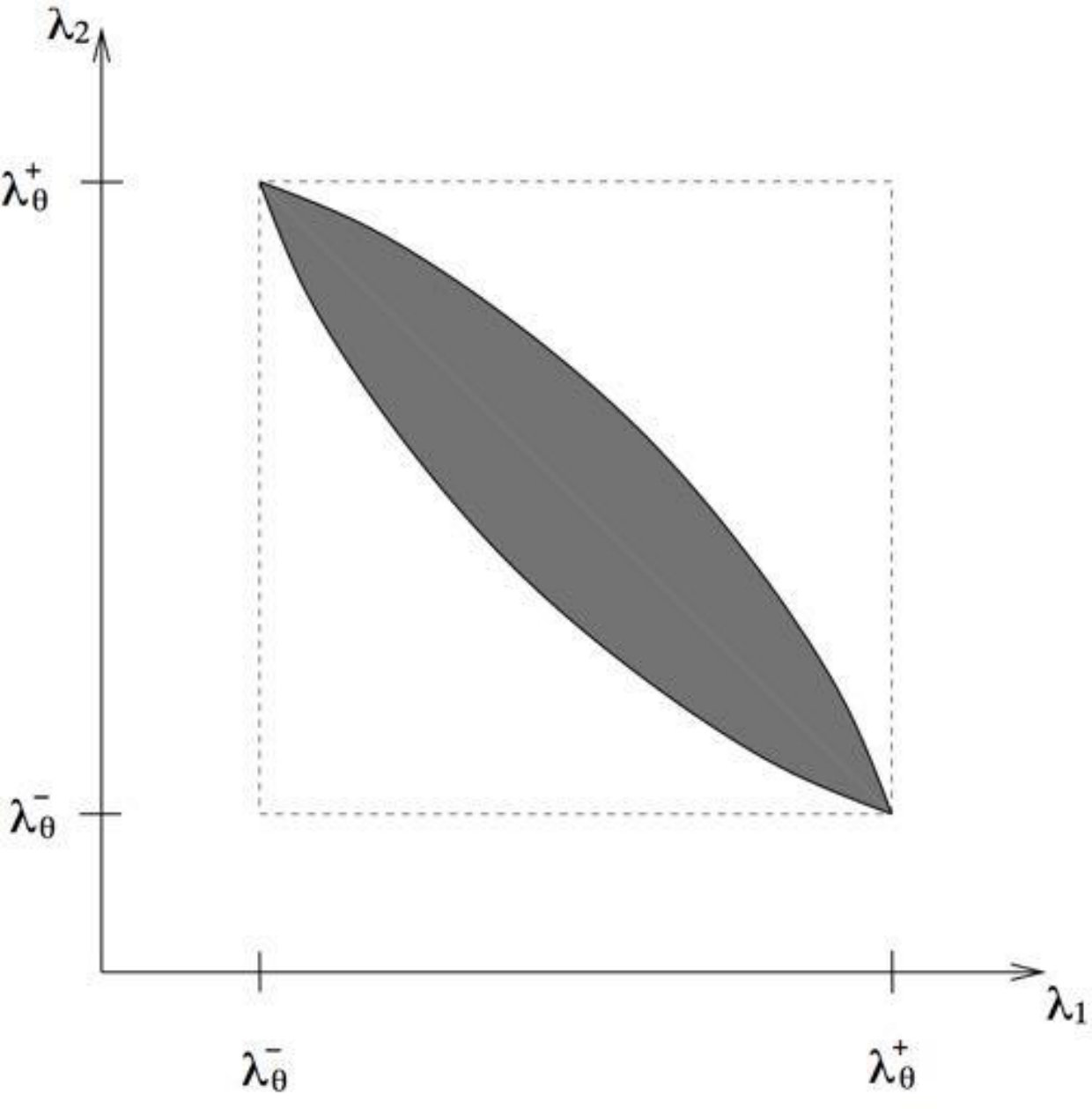 Figure 1
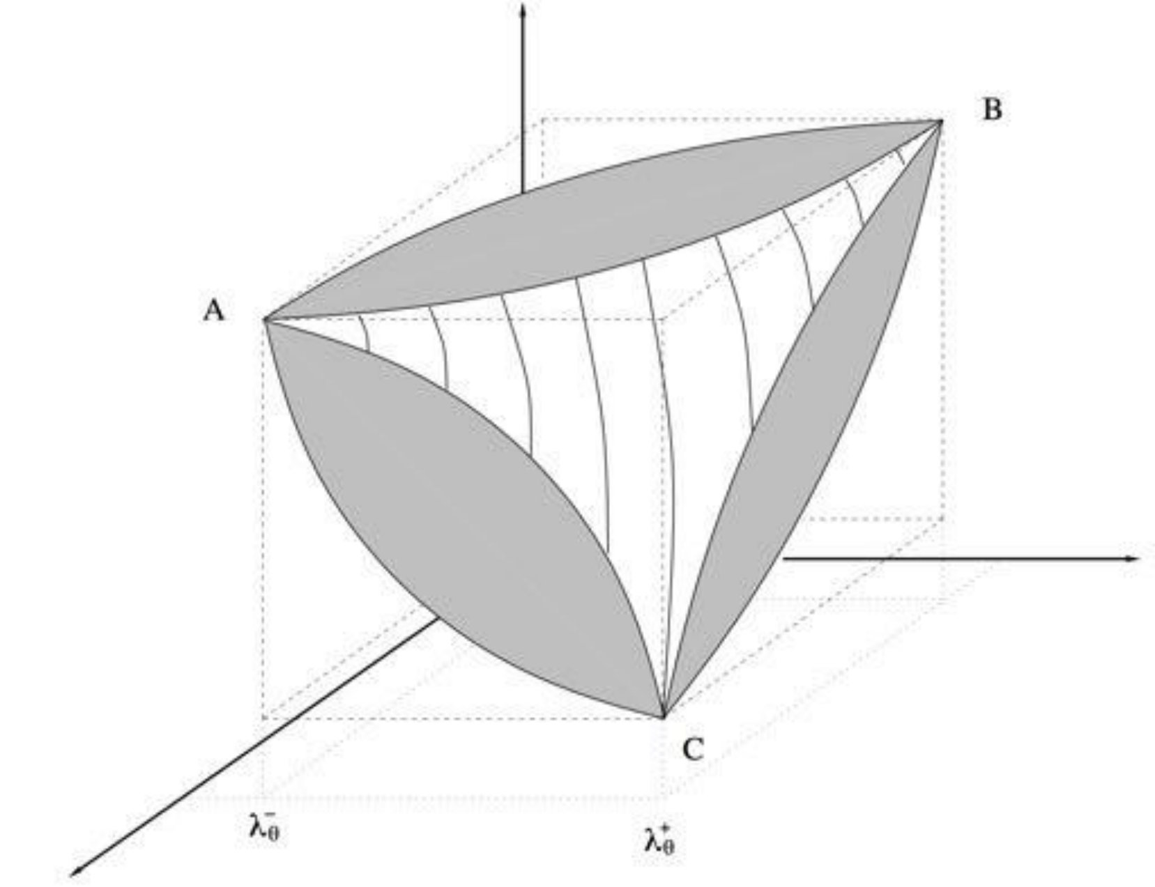 Figure 2
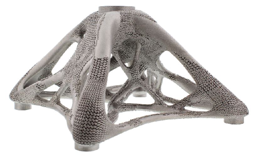 Figure 3
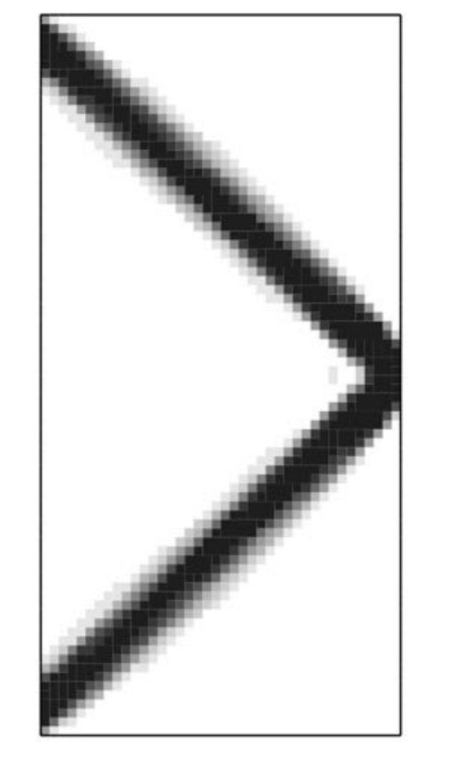 Figure 4
 Figure 5
 Figure 6
 Figure 7
 Figure 8
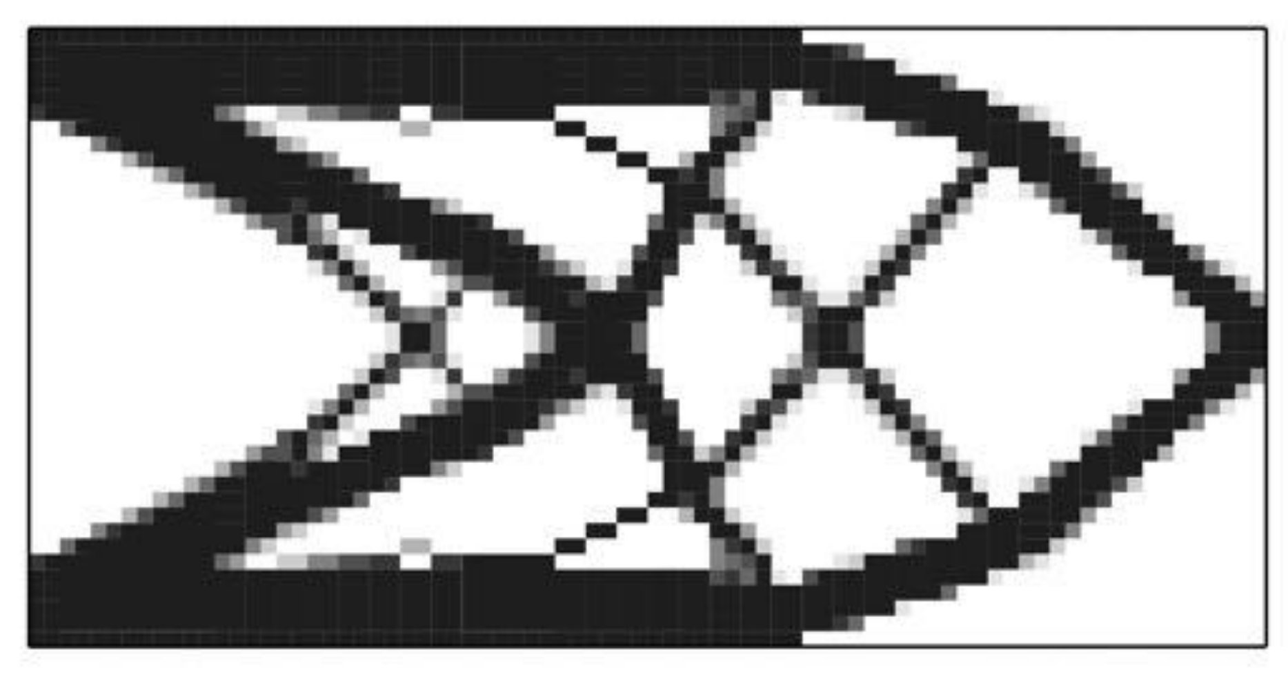 Figure 9
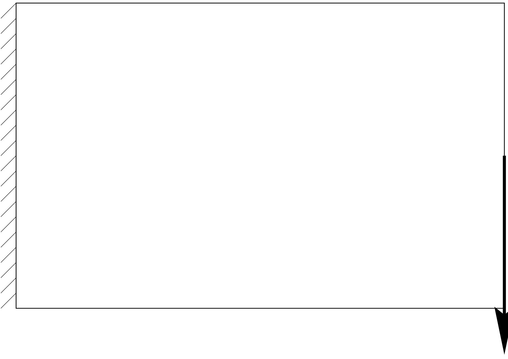 Figure 10
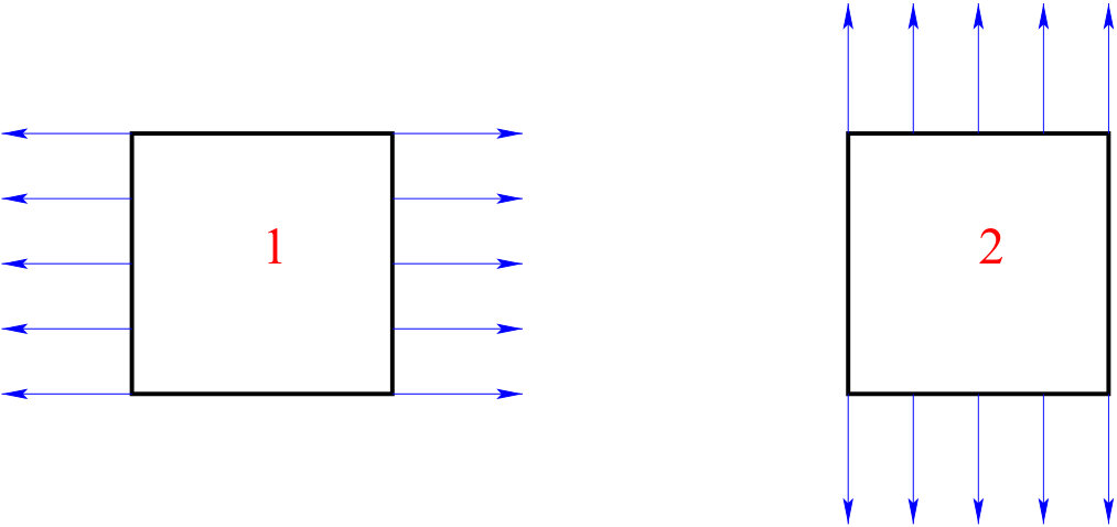 Figure 11
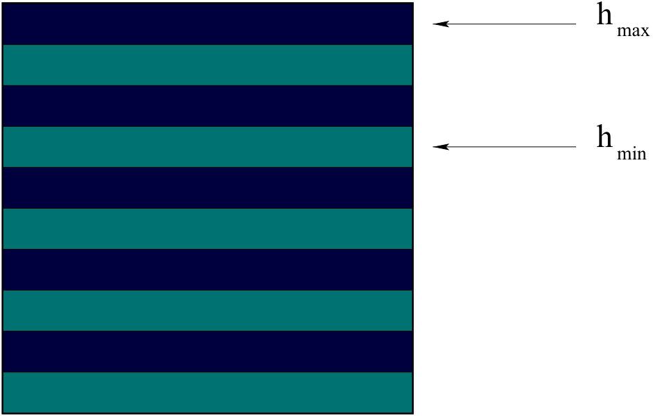 Figure 12
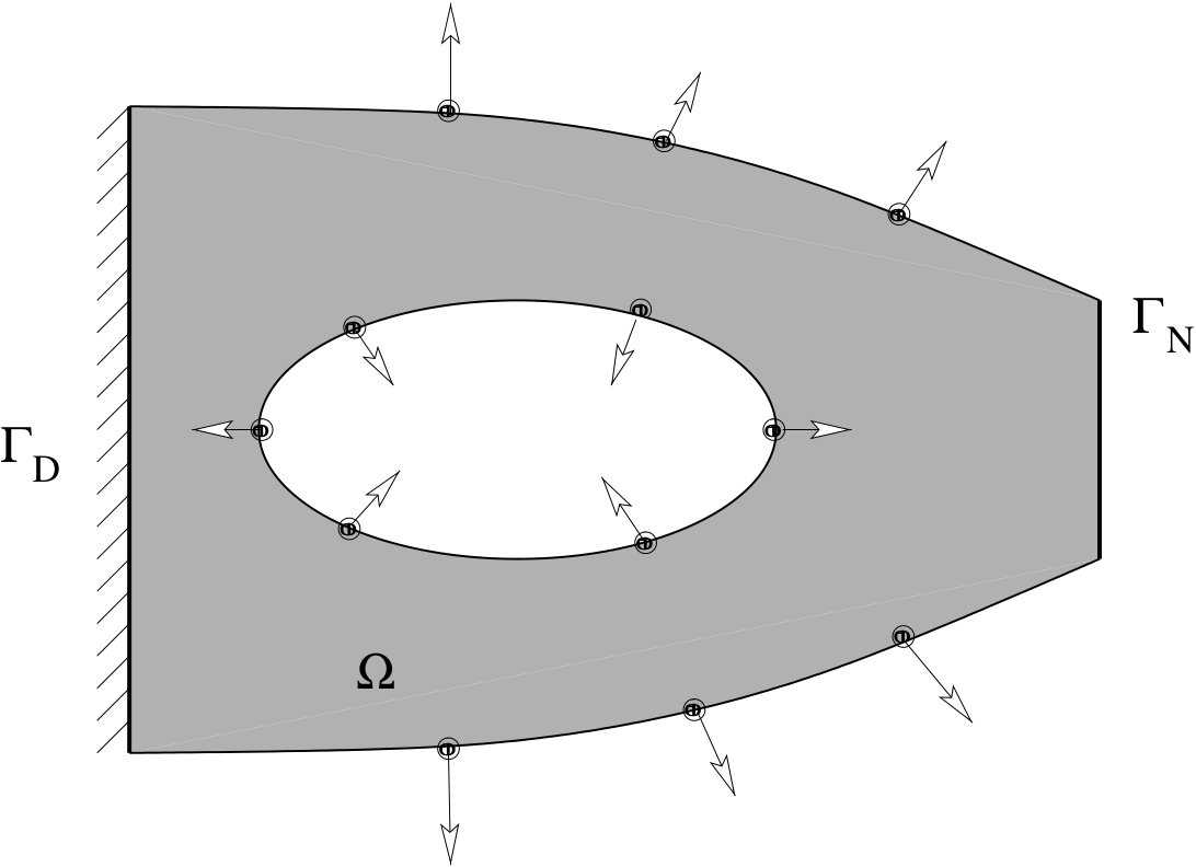 Figure 13
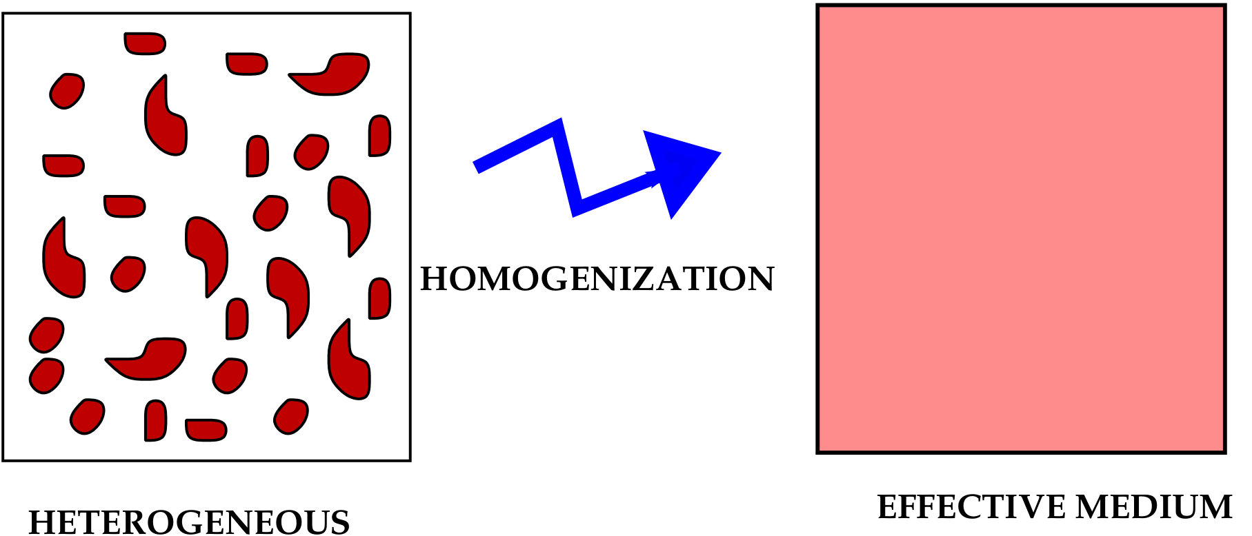 Figure 14
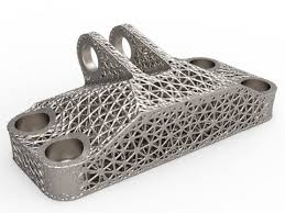 Figure 15
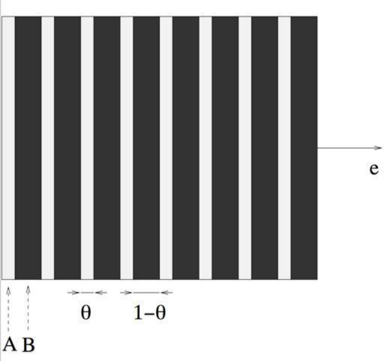 Figure 16
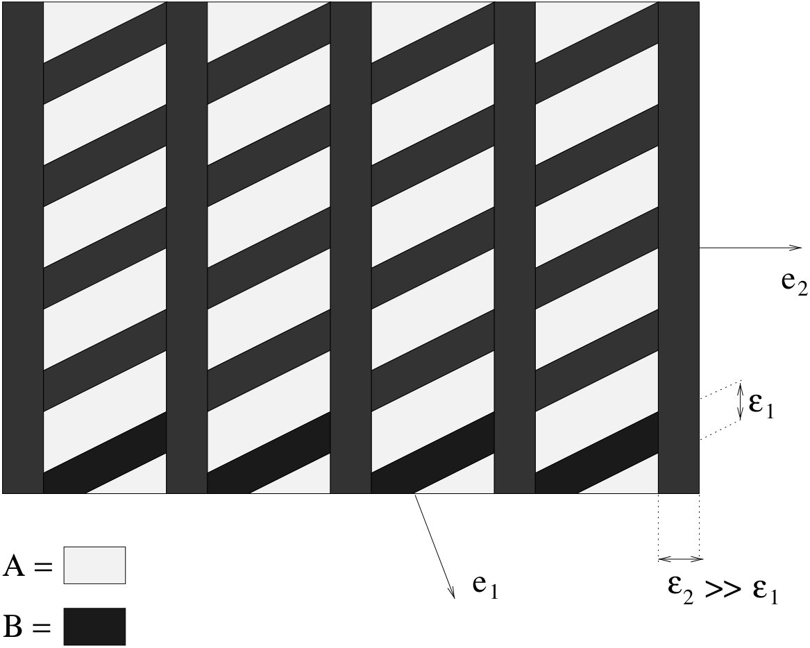 Figure 17
 Figure 18
 Figure 19
 Figure 20
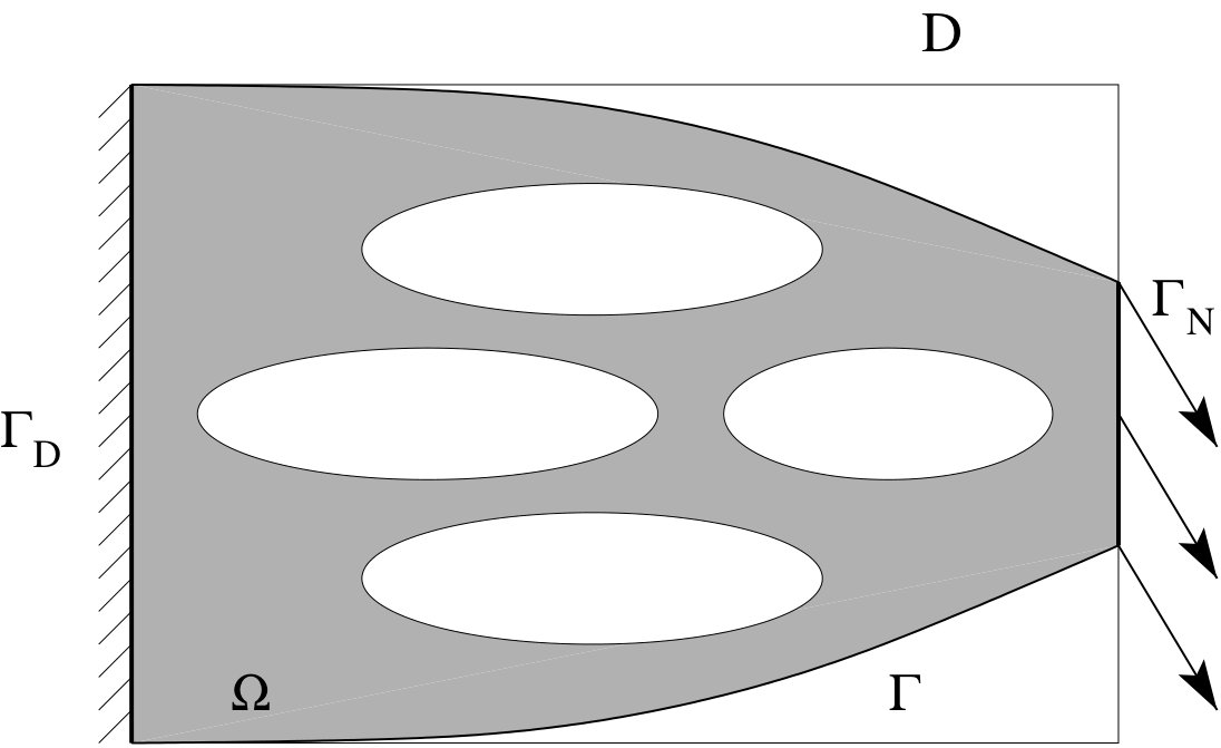 Figure 21
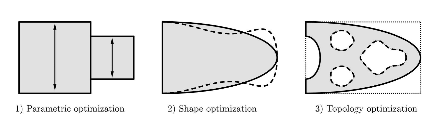 Figure 22
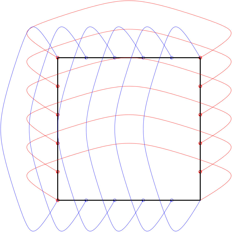 Figure 23
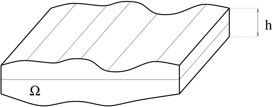 Figure 24
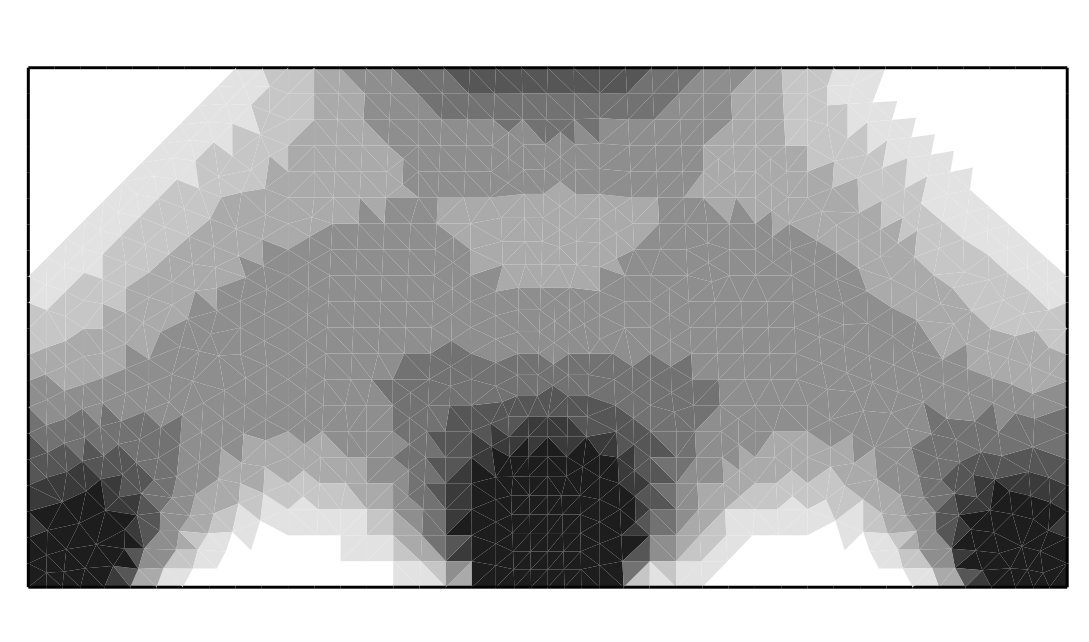 Figure 25
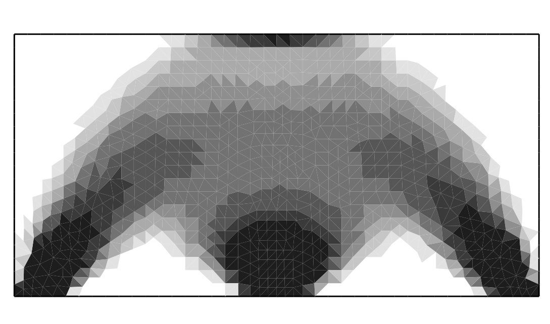 Figure 26
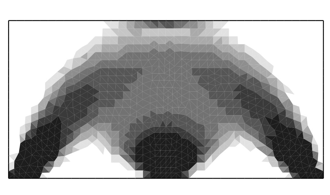 Figure 27
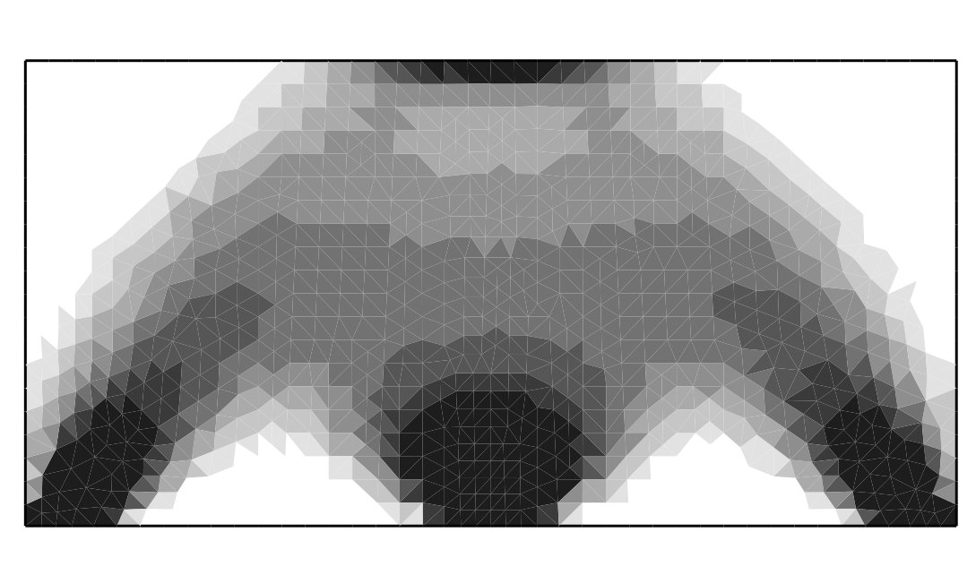 Figure 28
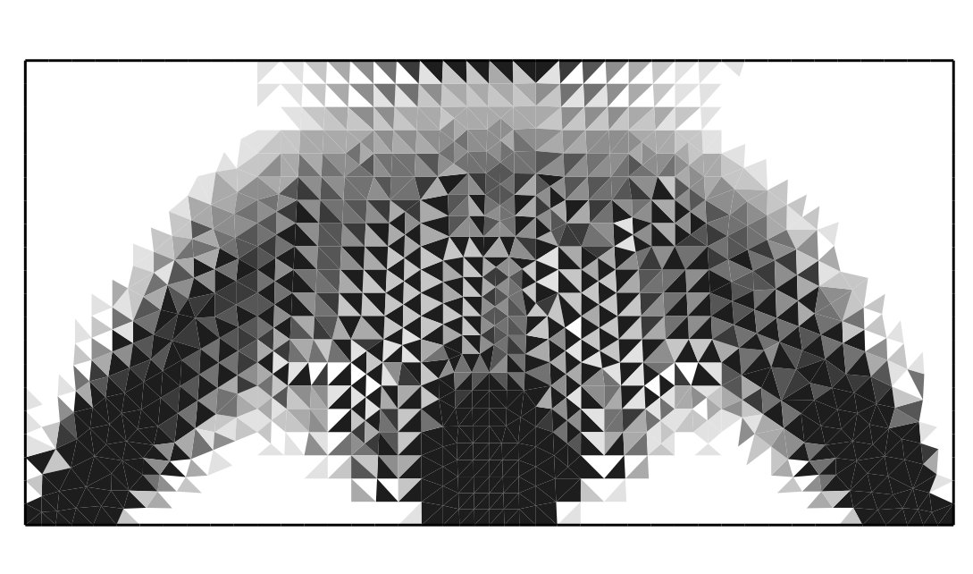 Figure 29
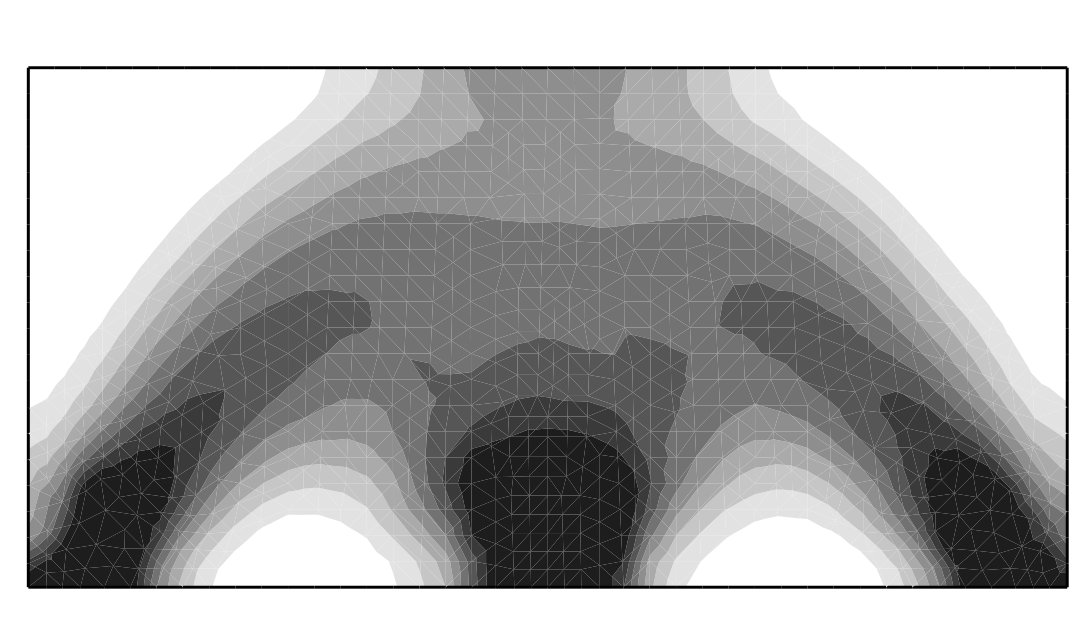 Figure 30
 Figure 31
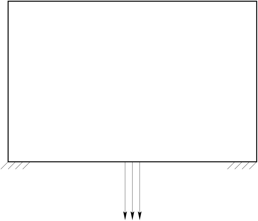 Figure 32
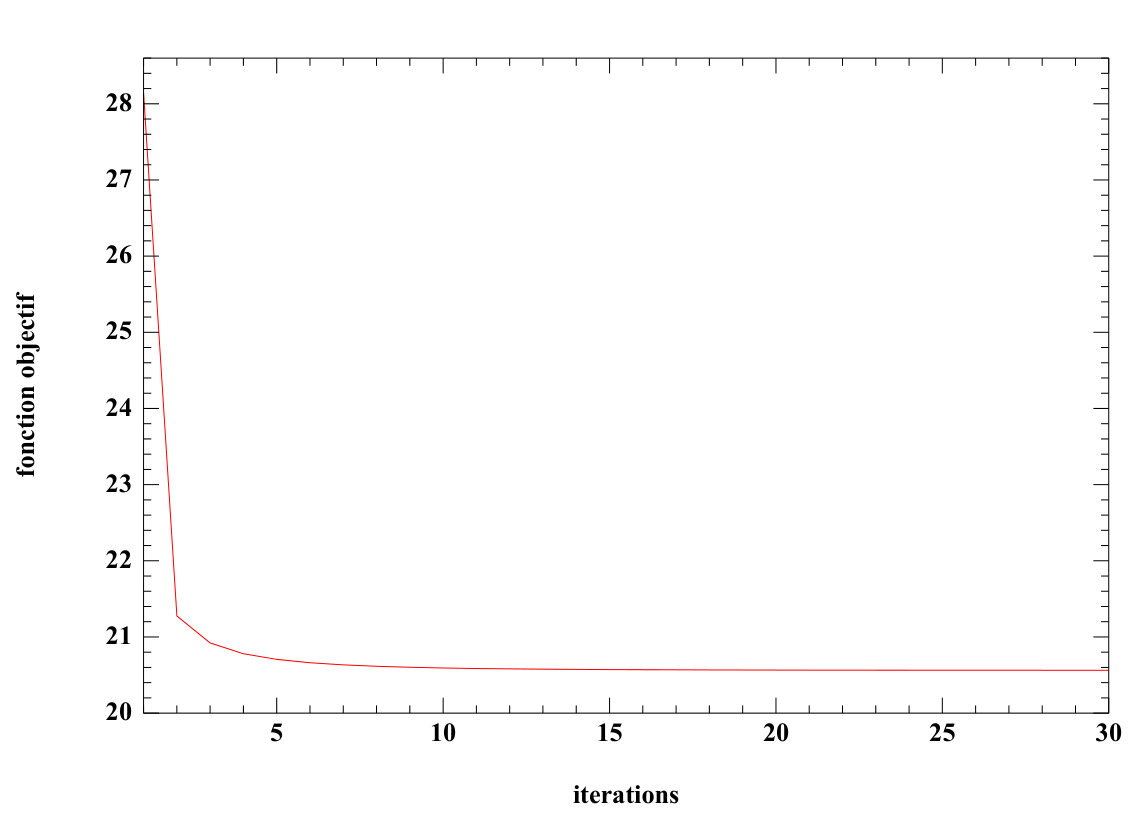 Figure 33
 Figure 34
 Figure 35
 Figure 36
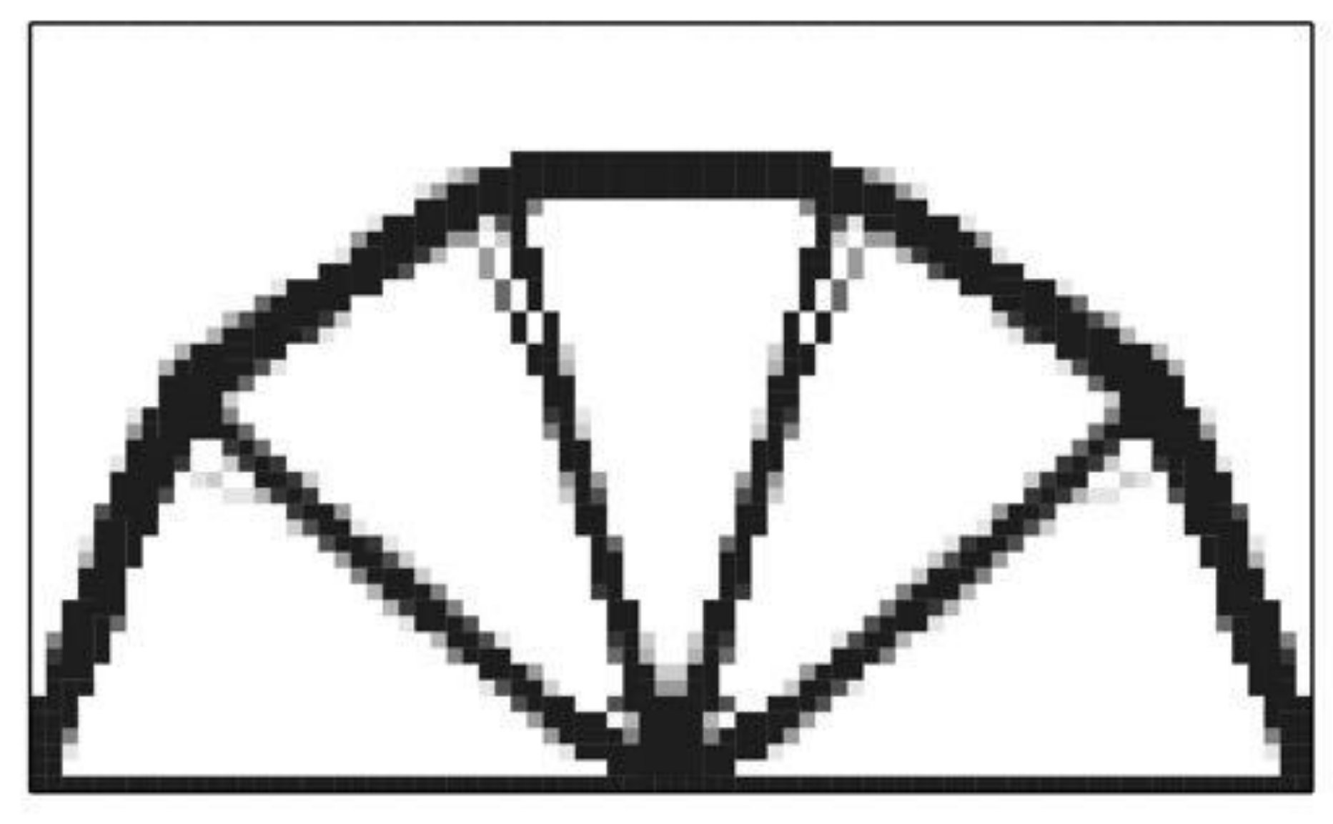 Figure 37
 Figure 38
 Figure 39
 Figure 40
Peer Reviews
No public reviews on file for this paper yet. If you reviewed it on a platform where reviews are public (OpenReview, ICLR, NeurIPS, ICML), you can paste yours below so the community can read it here.
Videos
No videos yet. Explain this paper in a talk, walkthrough, or lecture? Add one.
The homogenization method for topology optimization of structures: old and new
Grégoire Allaire
Lorenzo Cavallina
Nobuhito Miyake
Tomoyuki Oka
Toshiaki Yachimura
Grégoire Allaire
CMAP
Ecole Polytechnique,
Palaiseau, France
Lorenzo Cavallina
RCPAM, Graduate School of Information Sciences, Tohoku University,
980-8579 Sendai, Japan
Nobuhito Miyake
Mathematical Institute,
Tohoku University,
980-8578 Sendai, Japan
Tomoyuki Oka
Mathematical Institute,
Tohoku University,
980-8578 Sendai, Japan
Toshiaki Yachimura
RCPAM, Graduate School of Information
Sciences, Tohoku University,
980-8579 Sendai, Japan
Contents
-
5.3.1 Introduction of the model of the elasticity and relaxed problem
-
6 Resurrection of the homogenization method: lattice materials in additive manufacturing
-
6.5 2nd step: parametric optimization of the homogenized problem
-
6.6 3rd step: reconstruction of an optimal periodic structure
-
6.6.1 Projection in the simple case without varying orientation,
-
6.7 A final post-processing/cleaning of the lattice reconstruction
Preface and acknowledgments
These are the lecture notes of a short course on the homogenization method for topology optimization of structures, given by one of us, Grégoire Allaire, during the “GSIS International Summer School 2018” at Tohoku University (Sendai, Japan). Based on the slides of this course, the four other authors, Lorenzo Cavallina, Nobuhito Miyake, Tomoyuki Oka, Toshiaki Yachimura, have written the present lecture notes, which have been proofread by Grégoire Allaire. Each chapter of these lecture notes corresponds to one class, except the two first ones which were taught together.
Topology optimization of structures is nowadays a well developed field with many different approaches and a wealth of applications. One of the earliest method of topology optimization was the homogenization method, introduced in the early eighties. It became extremely popular in its over-simplified version, called SIMP (Solid Isotropic Material with Penalization), which retains only the notion of material density and forgets about true composite materials with optimal (possibly non isotropic) microstructures. However, the appearance of mature additive manufacturing technologies which are able to build finely graded microstructures (sometimes called lattice materials) drastically changed the picture and one can see a resurrection of the homogenization method for such applications. Indeed, homogenization is the right technique to deal with microstructured materials where anisotropy plays a key role, a feature which is absent from SIMP. Homogenization theory allows to replace the microscopic details of the structure (typically a complex networks of bars, trusses and plates) by a simpler effective elasticity tensor describing the mesoscopic properties of the structure.
The goal of this course is to review the necessary mathematical tools of homogenization theory and apply them to topology optimization of mechanical structures. The ultimate application, targeted in this course, is the topology optimization of structures built with lattice materials. Practical and numerical exercises are given, based on the finite element free software FreeFem++.
Finally, the authors would like to express their gratitude to the organizers of the Summer School: Reika Fukuizumi, Kei Funano, Jun Masamune, Jinhae Park, Ruo Li, Shigeru Sakaguchi, Kenjiro Terada, Takayuki Yamada and Lei Zhang. The meeting was partially supported by a grant from the JSPS A3 Foresight Program, JSPS KAKENHI Grant Numbers and , GSIS and RCPAM.
Chapter 1 Introduction
1.1 Optimal design of structures
A problem of optimal design (material, shape and topology optimization) of structures is defined by three ingredients (see [Al2007-1, BS2003, HM2003, HP2018, KPTZ2000, SK1992]):
- (a)
a model (typically a partial differential equation) to evaluate (or analyze) the mechanical behavior of a structure, 2. (b)
an objective function which has to be minimized or maximized, or sometimes several objectives (also called cost functions or criteria), 3. (c)
a set of admissible designs which precisely defines the optimization variables, including possible constraints.
The kind of optimal design problems which we focus on in these lecture notes can be roughly divided into three categories, from the “easiest” to the “most difficult” one:
Parametric or sizing optimization, for which designs are parametrized by a few variables (for example, thickness or member sizes), implying that the set of admissible designs is considerably simplified (see Figure 1-1, where the variable parameters, the thickness of the two boxes in this case, are symbolized by arrows), 2. 2.
Shape (geometric) optimization, for which all designs are obtained from an initial guess by moving its boundary without change of its topology due to the generation of new boundaries (see Figure 1-2, where an admissible shape is drawn with a broken line), 3. 3.
Topology optimization where both the shape and the topology of the admissible designs can vary without any explicit or implicit restrictions (see Figure 1-3, where the broken lines show removable holes).
The last category in the above is, of course, the most general but also the most difficult. We recall that two shapes share the same topology if there exists a continuous deformation from one to the other. In dimension , topology is completely characterized by the number of holes (or, equivalently, of connected components of the boundary). In dimension it is quite more complicated. Indeed, the topology of a set in dimension is not only determined by the number of holes, but it also depends on the number and intricacy of “handles” or “loops”.
First of all, one could ask theoretical questions concerning existence, uniqueness, and qualitative properties of the solutions of these shape optimization problems. One could also study the necessary and/or sufficient conditions satisfied by the optimal shapes. Such “optimality conditions” are very important both from a theoretical and a numerical point of view. They are often the basis for numerical algorithms of gradient method type. Furthermore one can investigate the numerical computation of approximate optimal shapes. All these questions will be addressed in the following chapters.
1.2 Example of sizing or parametric optimization
First of all, we show some examples of sizing or parametric optimization. Let us consider the thickness optimization of a membrane, where is a mean surface of a (plane) membrane and is the thickness in the normal direction to the mean surface (see Figure 2).
In what follows, we consider our membrane to be pre-stressed at its boundary and subject to some vertical force . Moreover, for small displacements, small deformations and negligible bending effects in the elasticity, the membrane deformation can be modeled by its vertical displacement , solution of the following partial differential equation, the so-called membrane model (see also [Al2007-1, K2016]),
[TABLE]
where the thickness is bounded by some given minimum and maximum values:
[TABLE]
The thickness is the optimization variable. Notice that we are dealing with a sizing or parametric optimal design problem here, because the computational domain does not change.
Let us define the set of admissible thickness as follows:
[TABLE]
where is an imposed average thickness.
Remark 1.1** (Possible additional “feasibility” constraints).**
According to the production process of membranes, the thickness can be discontinuous, or on the contrary continuous. A uniform bound can be imposed on its first derivative (molding-type constraint) or on its second order derivative , linked to the curvature radius (milling-type constraint).
The optimization criterion is linked to some mechanical property of the membrane, evaluated through its displacement , solution of the PDE,
[TABLE]
where, of course, depends on . For example, the global rigidity of a structure is often measured by its compliance, or work done by the load : the smaller the work, the larger the rigidity (compliance = rigidity). In such a case, we set
[TABLE]
Another example amounts to achieve (at least approximately) a target displacement , which is modeled by taking
[TABLE]
Those two criteria are the typical examples studied in this course. Then, a parametric optimization problem is
[TABLE]
Other examples of objective functions are the following:
- •
Introducing the stress vector , we can minimize the maximum stress norm
[TABLE]
or more generally, for any , the following -norm
[TABLE]
- •
For a vibrating structure, introducing the first eigenfrequency , defined by
[TABLE]
We consider to maximize it.
- •
Multiple loads optimization: for given loads the independent displacements are solutions of
[TABLE]
We then introduce an aggregated criterion
[TABLE]
with given coefficients , or
[TABLE]
1.3 Example of shape optimization
In this section, we show two examples of shape optimization. At first let us consider a shape optimization of a membrane’s shape. A reference domain for the membrane is denoted by , with a boundary made of three disjoint parts
[TABLE]
where is the variable part, is the Dirichlet (clamped) part and is the Neumann part (loaded by ).
The vertical displacement is the solution of the following membrane model
[TABLE]
From now on the membrane thickness is fixed, equal to . Moreover, we consider the parts and to be given. Thus the set of admissible shapes is
[TABLE]
where is a given volume. The shape optimization problem reads
[TABLE]
with, as a criterion, the compliance
[TABLE]
or a least-square functional to achieve a target displacement
[TABLE]
Notice that the true optimization variable is only the free boundary , and therefore the topology of the shape does not change.
Another example is a shape optimization in the elasticity setting. The model of linearized elasticity gives the displacement vector field as the solution of the system of equations
[TABLE]
with and , where and are the Lamé coefficients, and is the outer unit normal to . The boundary is again divided into three disjoint parts
[TABLE]
where is the free boundary, the true optimization variable. The set of admissible shapes is again
[TABLE]
where is a given imposed volume. The objective function chosen is either the compliance
[TABLE]
or a least-square criterion for the target displacement
[TABLE]
As before, the shape optimization problem reads
[TABLE]
1.4 Topology optimization and the homogenization method
In topology optimization, not only the connected components of the boundary are allowed to move but also new connected components (holes in -d) of can appear or disappear. Topology is now optimized too. In order to solve this task, we introduce the homogenization method. The homogenization method is a kind of averaging methods for partial differential equations, and is commonly used to determine the averaged (or effective, or homogenized, or equivalent, or macroscopic) parameters of a heterogeneous medium [Al2002, BLP1978, ch1000, CD1999, JKO1995, MT1997, TA2000].
How does homogenization apply to optimal design ? The homogenization method is based on the concept of “relaxation”: it makes ill-posed problems well-posed by enlarging the space of admissible “shapes”. It is crucial to introduce “generalized” shapes, that are “not too generalized”. In the homogenization method, we think of generalized shapes as “limits” of minimizing sequences of classical shapes. We can then say that homogenization allows, as admissible shapes, composite materials obtained by micro-perforation of the original material (fine mixtures of material and void).
1.5 Lattice materials in additive manufacturing
Additive manufacturing, also known as 3D printing, is a process that creates physical structures built layer by layer from a digital design by using metallic powder melted by a laser or an electron beam [GRS2015]. One of the main advantages of additive manufacturing is that, a priori, there are no limitations on the structures that can be built (unfortunately, in practice there are some limitations of manufacturability, like overhangs or the possibility of thermal residual stresses). Moreover, one can even build microstructures or lattice materials.
However, it is impossible to describe all the fine details of a lattice structure in a finite element model for optimization purposes. Therefore, homogenization theory is the right tool for dealing with lattice materials and related optimal design problems. In chapter 6, we will tackle the problem of optimizing lattice structures by using the homogenization method.
1.6 Goals of these lecture notes
The main goal of these lecture notes is to introduce the homogenization method for topology optimization of structures. The rest of these lecture notes are organized as follows. In chapter 2, we show some tools in optimization and describe numerical algorithms for computing optimal designs. In chapter 3, we consider parametric optimization problem and compute gradients of objective functions (by an optimal control approach) for further use in gradient-type algorithms. A representative example of parametric optimization is that of a membrane’s thickness. In chapter 4, we provide a brief survey on homogenization theory. In chapter 5, we apply the homogenization method to topology optimization. In chapter 6, we present a resurrection of the homogenization method for the design of lattice materials in additive manufacturing.
Through these lecture notes, numerical exercizes are proposed with the FreeFem++ code (http://www.freefem.org). FreeFem++ is a free software for solving partial differential equations by the finite element method [He2012]. Moreover, you can find some scripts of FreeFem++ for shape optimization in the web site (http://www.cmap.polytechnique.fr/~allaire/freefem_en.html) and in the corresponding educational paper [AP2006].
1.7 Exercises
Problem 1.7.1**.**
Solve (with FreeFem++) the elasticity equations for the following test cases: cantilever, bridge, MBB beam and L-beam (see Figure 7).
Chapter 2 Some tools in optimization
We review some classical result in optimization theory. More details can be found in textbooks like [Al2007-2, BGLS2006, ET1999, NW1999].
2.1 Generalities
Let be a Banach space and be a non-empty subset. Let . We consider the following minimization problem
[TABLE]
Let us specify some basic definitions.
Definition 2.1**.**
An element is called a local minimizer of on if
[TABLE]
Moreover, an element is called a global minimizer of on if
[TABLE]
Definition 2.2**.**
A minimizing sequence of a function on the set is a sequence such that
[TABLE]
By definition of the infimum value of on there always exists at least one minimizing sequence for on .
Let us consider the existence of minima for optimization problems in finite dimension. The following result guarantees the existence of a minimum.
Theorem 2.3**.**
Let be a non-empty closed subset of and a continuous function from to satisfying the so-called “infinite at infinity” property, i.e.,
[TABLE]
Then there exists at least one minimizer of on . Furthermore, from each minimizing sequence of over one can extract a subsequence which converges to a minimum of on .
Proof.
Let be a minimizing sequence for over . In particular, since is infinite at infinity and the sequence is bounded, we conclude that must be bounded as well. Therefore, since closed bounded sets are compact in finite dimension, there exists a subsequence that converges to a point . Now, because is closed, and converges to by continuity. We conclude that .
∎
Remark 2.4**.**
In an infinite dimensional vector space, a continuous function on a closed bounded set does not necessarily attain its minimum. For example, let be the usual Sobolev space with the norm . Let
[TABLE]
One can check that is continuous and “infinite at infinity”. Nevertheless the minimization problem
[TABLE]
does not admit a minimizer. Indeed, there exists no such that but, still,
[TABLE]
To obtain it, we construct a minimizing sequence defined for, , by
[TABLE]
as Figure 8.
We can easily check that and . Consequently,
[TABLE]
We clearly see in this example that the minimizing sequence is “oscillating” more and more and it is not compact in despite being bounded in the same space.
2.2 Convex analysis
As we have seen in Remark 2.4, continuous functions do not necessarily attain their minimum on a bounded closed set. In order to extend the result of Theorem 2.3 to the case of an infinite dimensional Hilbert space, we shall work in a convex framework.
Definition 2.5**.**
A set is said to be convex if, for any and for any , the linear combination belongs to .
Definition 2.6**.**
A function , defined from a non-empty convex set into is convex on if
[TABLE]
Furthermore, is said to be strictly convex if the inequality above is strict whenever and .
Theorem 2.7**.**
Let be a non-empty closed convex set in a reflexive Banach space (i.e. the dual of is itself), and be a convex continuous function on , which is “infinite at infinity”, i.e.,
[TABLE]
Then, there exists a minimizer of in .
Remark 2.8**.**
Theorem 2.7 remains true if is just the dual of some separable Banach space. In particular it holds true when with .
The proof will follow along the same lines as that of Theorem 2.3. However, the infinite dimensional case is much more delicate, since it relies on weak convergence and its relations with convexity. We refer to [Al2007-2, Theorem 9.2.7 and Remark 9.2.9] for a complete proof.
Proposition 2.9**.**
Under the hypotheses of Theorem 2.7, suppose that is strictly convex. Then has at most one minimizer.
Proof.
Suppose by contradiction that are two distinct minimizers of over the closed strictly convex set . If we take in (2.1), then we get
[TABLE]
which is contradicts the definition of minimum. ∎
Proposition 2.10**.**
If is convex on the convex set , then any local minimizer of on is a global minimizer.
Proof.
Let be a local minimizer of on . Thus there exists such that for any . Let . Our aim is to show that . Let be such that . For example we can take . Since , it follows that , and by Jensen’s inequality
[TABLE]
Thus, follows. ∎
Convexity is not the only tool to prove existence of minimizers. Another method is, for example, compactness.
2.3 Optimality conditions
In this section, we discuss optimality conditions for objective functions.
Definition 2.11**.**
Let be a Banach space. A function , defined from a neighborhood of into , is said to be differentiable in the sense of Fréchet at if there exists such that
[TABLE]
We call the differential (or derivative, or gradient) of at and we denote it by
[TABLE]
Remark 2.12**.**
If is a Hilbert space, its dual can be identified with itself thanks to the Riesz representation theorem. Thus, there exists a unique such that . We also write . We use this identification if or . In practice, it is often easier to compute the directional derivative with .
Consider the variational formulation
[TABLE]
where is a symmetric coercive continuous bilinear form and is a continuous linear form. By the Lax–Milgram theorem we know that the variational formulation (2.3) admits a unique solution. Let us now define the energy
[TABLE]
The following lemma tells us the relationship between the energy and the variational formulation (2.3).
Lemma 2.13**.**
Let be the unique solution of the variational formulation (2.3). Then is the unique minimizer of , that is,
[TABLE]
Conversely, if is a point giving an energy minimum of , then is the unique solution of the variational formulation (2.3).
Proof.
If is the solution of the variational formulation (2.3), then thanks to the symmetry of we have
[TABLE]
As is arbitrary in , minimizes the energy in .
Conversely, let be such that
[TABLE]
For we define . Then
[TABLE]
We differentiate ,
[TABLE]
By definition, , thus
[TABLE]
Since is a minimum point of , we have for all . ∎
Remark 2.14**.**
When computing the Fréchet differential of a given functional at (see the definition of and in (2.2)), there is not always an obvious way to deduce a formula for , nevertheless most of the time it is enough to know the mapping .
Example 2.15**.**
For fixed , define
[TABLE]
We have
[TABLE]
Thus
[TABLE]
Notice that here we identified with its dual. 2. 2.
For fixed define
[TABLE]
We have
[TABLE]
Therefore, by the usual definition of the duality pairing between and (that comes from a formal integration by parts) we get
[TABLE]
Notice that here the space is not identified with its dual.
Remark 2.16**.**
If instead of the “usual” scalar product in we rather use the scalar product in the second part of Example 2.15, then we have to identify with a different function (in other words, the definition of depends on the scalar product used). From the directional derivative
[TABLE]
using the scalar product , we deduce that
[TABLE]
in the distributional sense. Here we identify with its dual.
Theorem 2.17** (Euler inequality).**
Let be a convex Banach space. Take and let be differentiable at . If is a local minimizer of in , then
[TABLE]
On the other hand, if satisfies this inequality and is convex, then is a global minimizer of in .
Proof.
For and , we have . Thus, if is sufficiently small, since is a local minimizer of in , we have
[TABLE]
We obtain inequality (2.4) by letting in the above.
We will now prove the second claim of the theorem. Since, by hypothesis is convex on , then, the graph of always lies above its tangent plane at any point . In other words, the following inequality holds true for all :
[TABLE]
The conclusion follows by taking . ∎
Remark 2.18**.**
If belongs to the interior of , then we deduce the Euler equation .
Remark 2.19**.**
The Euler inequality is usually just a necessary condition (for instance, it is verified also if is a local maximizer). It becomes a necessary and sufficient condition under the further assumption that the functional is also convex.
2.3.1 Minimization with equality constraints
We consider the following problem
[TABLE]
where is a differentiable function from into .
Notice that the set is not necessarily convex. We will therefore need a generalized version of the Euler inequality as stated in Theorem 2.17. To this end we introduce the set of admissible directions for our constrained optimization problem.
Definition 2.20**.**
At every point , the set
[TABLE]
is called the cone of admissible directions at the point .
In other words, is the set of all vectors that are tangent at to a curve in that passes through (hence, if is a regular manifold, coincides with the tangent space to at ). Moreover, notice that, as the name suggests, the set is a cone in the sense of convex analysis: namely, for all and , then also .
Proposition 2.21** (Euler inequality, general case).**
Let be a local minimum of over . Then, if is differentiable at , we have
[TABLE]
Proof.
With the same notations of Definition 2.20, set . By definition, we have that if and only if there exists a sequence in and a sequence of positive real numbers such that
[TABLE]
Now, since is a local minimum of over , we get
[TABLE]
Passing to the limit as yields
[TABLE]
as claimed. ∎
Definition 2.22**.**
We call Lagrangian of problem (2.5), the function
[TABLE]
The new variable is called Lagrange multiplier for the constraint .
Lemma 2.23**.**
The constrained minimization problem (2.5) admits the following equivalent formulation using the Lagrangian:
[TABLE]
Proof.
The proof is done by cases. Notice that, if , then for all . On the other hand, if , then . Putting the two together yields
[TABLE]
∎
Theorem 2.24** (Stationarity of the Lagrangian).**
With the same notation of (2.5), assume that and are continuously differentiable in a neighborhood of such that . If is a local minimizer and if the vectors are linearly independent, then there exist a Lagrange multiplier such that
[TABLE]
Proof.
First define and then the corresponding cone of admissible directions by Definition 2.20. Now, since the vectors are linearly independent by hypothesis, we can use the implicit function theorem in a standard way to deduce that
[TABLE]
or equivalently
[TABLE]
In particular is a vector space (it is indeed the tangent space to the variety at the point ). Thus we can successively take and in Proposition 2.21 to get
[TABLE]
This implies that is generated by (moreover, since the are linearly independent, the Lagrange multipliers are uniquely defined). ∎
2.3.2 Minimization with inequality constraints
We consider the following minimization problem with inequality constraints
[TABLE]
where here means that for , with differentiable.
Definition 2.25**.**
Let be such that . The set
[TABLE]
is called the set of active constraints at . The inequality constraints are said to be qualified at if the vectors are linearly independent.
There are other (more general) definitions of constraints qualification [BGLS2006].
Definition 2.26**.**
We call Lagrangian of the previous problem the function
[TABLE]
The new non negative variable is called Lagrange multiplier for the constraint .
The proof of the result below is analogous to that of Lemma 2.23 and thus will be omitted.
Lemma 2.27**.**
The constrained minimization problem (2.7) is equivalent to
[TABLE]
The existence of (non negative) Lagrange multipliers, analogous to Theorem 2.24, can be proved also for a minimization problem subject to inequality constraints. We refer to [Al2007-2, Theorem 10.2.15] for a proof.
Theorem 2.28** (Stationarity of the Lagrangian for the inequality constraint).**
We assume that the constraints are qualified at satisfying . If is a local minimizer, there exist Lagrange multipliers such that
[TABLE]
The condition (2.8) is indeed the stationarity of the Lagrangian since
[TABLE]
and the condition and for , is equivalent to the Euler inequality (Theorem 2.17) associated to the maximization problem with respect to the variable in the closed convex set . Indeed
[TABLE]
and thus for all as claimed.
2.3.3 Interpreting the Lagrange multipliers
Define the Lagrangian for the minimization of under the constraint as follows:
[TABLE]
We claim that the value of the Lagrange multiplier represents the sensitivity of the minimal value with respect to variations of the constraint . To this end, let and denote the minimizer and the optimal Lagrange multiplier respectively. Moreover, we assume that they are differentiable with respect to . Then
[TABLE]
In other words, gives the derivative of the minimal value with respect to without any further calculation. Indeed
[TABLE]
where, in the last equality we used
[TABLE]
which are a consequence of Theorem 2.24 and the constraint respectively.
2.4 Dual energy
In this section, we shall associate to a minimizing problem with a maximizing problem, so called dual problem. To simplify the argument, we will assume that and are two Banach spaces. Let and be the corresponding dual spaces. The following argument is according to [ET1999] and see the book for the more general setting. For , we consider the following minimizing problem:
[TABLE]
For given problem (2.9), we are now able to define a dual problem. We shall consider a function such that
[TABLE]
We define the conjugate function as
[TABLE]
We call the problem
[TABLE]
the dual problem of (2.9).
In the following, we will mention the relationship between (2.9) and (2.10) in a special case. Let be a continuous linear operator. Assume that can be rewritten as
[TABLE]
where is a function of into . In this case, the function will be
[TABLE]
Then the conjugate function becomes
[TABLE]
For this case, we can see the following relationship.
Theorem 2.29**.**
Assume that is convex and (2.9) is finite. We also assume that there exists such that and the function is continuous at . Then
[TABLE]
and maximizing problem (2.10) has at least one solution.
To show Theorem 2.29, we will use convex analysis. For the details of the proof, see [ET1999, Chapter III, Theorem 4.1].
Example 2.30**.**
We show an application of Theorem 2.29. Let be a smooth domain. We consider the Dirichlet problem
[TABLE]
where and is a positive given function. The solution of the problem above is the minimizer of
[TABLE]
We can apply Theorem 2.29 with
[TABLE]
In the case, we see that
[TABLE]
and hence
[TABLE]
2.5 Numerical algorithms
In this section we present some numerical algorithms in order to solve the kind of minimization problems that were treated in this chapter. All these algorithms are of iterative nature: starting from a give initial value , we construct a sequence , which can be shown to converge to the solution of the given minimization problem under some hypotheses.
2.5.1 A gradient-type algorithm (non-constrained case)
Suppose that (or, more generally, a Hilbert space, that we will identify with its dual ). We consider the following minimization problem without constraints:
[TABLE]
We initialize the algorithm by choosing some initial value and iteratively update it as follows:
[TABLE]
where is a positive parameter that we choose in advance (a more sophisticate algorithm involving the optimal choice of for each iteration is discussed in [Al2007-1, Theorem 3.38]).
Theorem 2.31**.**
Let be a Hilbert space and suppose that the functional is strongly convex, that is, for some
[TABLE]
Moreover, assume that is differentiable with Lipschitz continuous derivative . Then, if is small enough (depending on and on the Lipschitz constant of ), the gradient-type algorithm described above converges. In other words, for all , the sequence defined in (2.12) converges to the solution of (2.11).
For a proof, see [Al2007-2].
Remark 2.32**.**
Choosing the right step length is not an easy task. Let us use the line search strategy as follows: start with a given step . Now, at each iteration, increase the current step, , if decreases, and reduce it, if increases.
2.5.2 A gradient-type algorithm (constrained case)
Suppose that is a real valued strictly convex differentiable functional defined on a nonempty closed convex subset of the Hilbert space . The set represents the imposed constraints. We consider the following minimization problem
[TABLE]
Theorem 2.3 ensures the existence of a minimizer for (2.13) (which is unique by Proposition (2.9)). Moreover, according to Theorem 2.17, the minimizer is characterized by the condition
[TABLE]
Notice that the condition above can be rephrased as follows. For all
[TABLE]
Let denote the projection operator onto the convex subset . Then (2.14) just states that is the orthogonal projection of onto . In other words
[TABLE]
Therefore we devise a (projected) gradient-type algorithm, defined by the following iteration
[TABLE]
where is a fixed positive parameter.
Theorem 2.33**.**
Let be a differentiable strongly convex functional, with derivative Lipschitz continuous on . Then, if is small enough, the projected gradient algorithm with fixed step defined above converges. In other words, for all initial values , the sequence defined by (2.15) converges to the solution of (2.13).
We refer to [Al2007-2, Theorem 10.5.8] for a proof.
Remark 2.34**.**
Another possibility is to penalize the constraints, i.e., for small we replace the problem
[TABLE]
Example 2.35** (Some projection operators ).**
Here we present some projection operators that can be computed explicitly.
- •
If and , then for we have
[TABLE]
- •
If and \displaystyle K=\Big{\{}x\in\mathbb{R}^{M}\mathrel{\mathop{\mathchar 58\relax}}\;\sum_{i=1}^{M}x_{i}=c_{0}\Big{\}}, then
[TABLE]
- •
Similarly, if and or the corresponding projection operators can be obtained by replacing finite sums with integrals in the two examples above.
For more general closed convex sets , the corresponding projection operator can be very hard to determine. In such cases one can use the so called Uzawa algorithm [Al2007-2] which looks for a saddle point of the Lagrangian.
2.6 Exercises
Problem 2.6.1**.**
For a given , being a rectangle in 2D, solve the following optimization problem numerically under the constraints and :**
[TABLE]
Problem 2.6.2**.**
For a given , being a rectangle in 2D, and , solve the following optimization problem numerically under the constraints :**
[TABLE]
Chapter 3 Parametric optimal design
3.1 Optimization of a membrane’s thickness
In this section, we consider a parametric optimal design problem of a membrane. Let be a bounded domain in () and be external forces. Let us consider the displacement , defined as the solution of
[TABLE]
where is the thickness of membrane. Note that Lax–Milgram theorem ensures that there exists a unique solution of (3.1) if . For some given constants , we seek to optimize the membrane by varying its thickness in the admissible set defined by
[TABLE]
We consider the following parametric shape optimization problem:
[TABLE]
where depends on through the state equation (3.1), and is a function from to such that and . As examples of function , we can take if we want to minimize the compliance (maximize the rigidity of the membrane), or if we want to minimize the least-square criterion to reach a target displacement .
Before studying the existence of an optimal thickness, we show the continuity of the cost function.
Proposition 3.1**.**
The application
[TABLE]
is a continuous mapping from into .
Proof.
The result follows immediately by composition of the two continuous functions that appear in the following lemmas: Lemma 3.2 and Lemma 3.3. ∎
Lemma 3.2**.**
The map is continuous from into .
Proof.
The result follows by the Lebesgue dominated convergence theorem. ∎
Lemma 3.3**.**
The map , where is the solution of (3.1), is a continuous function from into .
Proof.
Let be a sequence converging in the -norm to some . Let denote the unique solution of the membrane equation with associated thickness :
[TABLE]
or the equivalent weak formulation
[TABLE]
We will prove that is a Cauchy sequence in and thus it converges. Take and subtract the variational formulation for (3.2) from that of for fixed to be chosen later. We get
[TABLE]
Choosing we deduce
[TABLE]
which proves the claim. ∎
3.2 Existence theories
The question of the existence of optimal shapes is far from simple. We cannot apply the results of Chapter 2 directly since is not generally convex function. In fact, there exists no optimal shape in general. General counter-examples have been found by Murat [Mu1977]. It is an important issue because this non-existence phenomenon has dramatic consequences for the numerical computations. Thus the definition of the set of admissible designs has to be modified in order to obtain existence of optimal shapes. The main strategies employed to gain the existence of optimal shapes are discretization (when the admissible set is made finite dimensional), regularization (when the admissible set is made compact), and sometimes a miracle (when the given optimization problem happens to be convex).
3.2.1 Definition of a counter-example
First, let us show a counter-example to the existence of optimal design for the membrane problem. For simplicity, let and .
We want to minimize the following objective function for :
[TABLE]
where , are the horizontal and vertical directions , respectively and , are the solutions of the following membrane problems:
[TABLE]
When we minimize (3.3), we want the membrane to be strong for horizontal loading (we minimize compliance in the direction), and at the same time weak for vertical loading (we maximize the compliance in the direction ). This property of the objective function makes the problem ill-posed in the following sense.
Theorem 3.4**.**
The infimum of (3.3) is not attained by any .
Since the rigorous proof of Theorem 3.4 is a little bit technical, here we will only explain the main ideas by means of a “hand-waving argument”. First of all, notice that if is uniform (i.e. is a constant function), then by definition the membrane is isotropic. Therefore, also the domain is isotropic, that is to say that it shows the same mechanical behavior in all direction. However, it is better to build horizontal layers of alternating small and large thicknesses in order to minimize the objective function (3.3) (see Figure 10). In other words, we are building a laminated structure that is horizontally strong but vertically weak. In order to intuitively justify this statement consider the following. Vertically, the lines of forces must cross the layers of minimal thickness: this means that the structure is thus weak with respect to vertical stress. On the other hand, horizontally, the lines of forces follow the layers of maximal thickness: this means that the structure is thus strong with respect to horizontal stress. However, since the boundary conditions are uniform, the membrane is horizontally stronger if the layers are finer, as the lines of forces are deviating from the horizontal to a lesser extent. If oscillates at a small scale, we obtain an anisotropic composite material. To reach the minimum, the oscillation scale must go to [math]. Therefore, there does not exist any real optimal design that does not involve a microstructure at an infinitely small scale. We refer the interested reader to Section 5.2 in [Al2007-1] for the details.
3.2.2 Existence for a discretized model
One way to avoid non-existence due to a loss of compactness consists in working with a discretized (and hence finite-dimensional) model. Let be a partition of such that
[TABLE]
We introduce the subset of defined by
[TABLE]
In other words, any function is uniquely determined by the choice of the vector and thus is identified with a closed subset of .
Theorem 3.5** (Existence in finite dimension).**
The discretized optimization problem
[TABLE]
admits at least one minimizer.
Proof.
Since is a compact subset of and is a continuous function on , the existence of a minimizer of in follows from Theorem 2.3. ∎
3.2.3 Existence with a regularity constraint
Another classical way of ensuring the existence of minimizers relies in imposing additional regularity. For example, consider the space which is a Banach space with the norm
[TABLE]
Take a given constant and introduce the subspace :
[TABLE]
The upper bound on the -norm of in the definition above can be interpreted as a “feasibility” (or “manufacturability”) constraint, as, in practice, the thickness cannot vary too rapidly. Then the following theorem holds:
Theorem 3.6**.**
The regularized optimization problem
[TABLE]
admits at least one minimizer.
Proof.
Consider a minimizing sequence such that
[TABLE]
By definition, the sequence is bounded uniformly in in the space . We then apply a variant of Rellich theorem which states that one can extract a subsequence (still denoted by for simplicity) that converges in to a limit function (furthermore, we know that ). We already know that is a continuous mapping from into by Proposition 3.1, therefore
[TABLE]
which proves that is a global minimizer of in as claimed. ∎
Remark 3.7**.**
Theorem 3.6 is actually a theorem of limited practical interest for the following reasons.
- •
In the practical cases, it is not clear how to choose the upper bound in the definition of .
- •
Usually we do not have convergence as goes to infinity.
- •
It is not clear whether, numerically, we have global or local minimizers.
- •
Numerically, an upper bound on the -norm is preferred instead:
[TABLE]
3.3 Computation of a continuous gradient
In this section, we will calculate the gradient of the objective function . This tells us the necessary conditions for optimality of the optimal shape and allows us to establish a numerical algorithm for calculating the optimal shape.
First, we consider the boundary value problem
[TABLE]
where belong to the following convex set which is larger than \mathcal{U}_{\rm ad}$$\colon
[TABLE]
Lemma 3.8**.**
The application , which gives the solution of (3.4) for , is differentiable and its directional derivative at in the direction is given by
[TABLE]
where is the unique solution in of
[TABLE]
Proof.
Formally, one simply differentiates equation (3.4) with respect to . However, to be mathematically rigorous one should rather work at the level of the variational formulation. To compute the directional derivative with respect to , we define for . For , let be the solution for the thickness . Differentiating with respect to leads to
[TABLE]
and, since , we deduce .
Let us justify the above calculation by showing that the map is differentiable in the sense of Fréchet. First, there exists a unique solution of (3.5) in thanks to the Lax–Milgram Theorem applied to the variational formulation
[TABLE]
We combine (3.6) with the following variational formulation for
[TABLE]
Since and , we obtain by difference
[TABLE]
Taking as a test function in the above yields
[TABLE]
which implies
[TABLE]
where we used Cauchy–Schwarz’s inequality and the boundedness of . Furthermore, by (3.7) we have
[TABLE]
Taking the test function as in (3.10), we obtain the following estimate:
[TABLE]
Combining (3.8) with (3.11), we have
[TABLE]
Therefore we obtain as , which proves the claim. ∎
Lemma 3.9**.**
For , let be the solution to (3.4) and
[TABLE]
where is a function from into such that and for any . The application , from into , is differentiable and its directional derivative at in the direction is given by
[TABLE]
where is the unique solution in of
[TABLE]
Proof.
By simple composition of differentiable applications. To justify it, one only has to check that all the terms are well defined. We omit the details of the proof. ∎
3.3.1 Adjoint state
In order to treat the derivative of the objective function , we introduce the adjoint state , defined as the unique solution in of
[TABLE]
Theorem 3.10**.**
The cost function is differentiable on and
[TABLE]
If is a local minimizer of in , then it satisfies the necessary optimality condition
[TABLE]
for any .
Proof.
To make explicit from Lemma 3.9, we must eliminate . To this end, we employ the use of the adjoint state, solution of (3.12). multiplying the equation for by and that for by , we integrate by parts
[TABLE]
[TABLE]
Comparing these two equalities we deduce
[TABLE]
for any . Since belongs to , we check that is continuous on . To obtain the condition of optimality, it suffices to apply Theorem 2.17 since is a closed non-empty convex subset of . ∎
Remark 3.11** (How to find the adjoint state).**
For independent variable , we introduce the Lagrangian
[TABLE]
where is a Lagrange multiplier (a function) for the constraint which connects to . By integration by parts we get
[TABLE]
The partial derivative of at in the direction is given by
[TABLE]
Notice that, requiring that for all directions is nothing else than the variational formulation of the adjoint equation (3.12).
3.3.2 A simple formula for the derivative
It is possible to compute the derivative of by means of the Lagrangian in the following way:
[TABLE]
where is the state function (solution to (3.4)) and is the adjoint state (solution to problem (3.12)). Indeed, we have
[TABLE]
by definition of the state function . Thus, if the map is differentiable, we get for
[TABLE]
Then, taking , the adjoint we obtain
[TABLE]
By the above discussion, we obtain the following theorem.
Theorem 3.12**.**
Let be the Lagrangian defined as the sum of the objective function and the variational formulation of the state equation, i.e.,
[TABLE]
Let be the solution of the adjoint equation
[TABLE]
Assume that the solution of the state equation (3.4) is differentiable with respect to . Then the objective function is differentiable and
[TABLE]
This theorem is the practical method for computing . Once the gradient of the cost function has been obtained, it is natural and quite easy to implement a gradient method to minimize numerically. In Section 3.5, we provide numerical algorithms to compute the optimal thickness.
3.4 A discrete approach
One can wonder whether the such optimal design problems get simpler after discretization. Unfortunately, the answer is “no”. In this section, we consider a discrete approach to the problems. Applying a finite element method, the equation becomes a linear system of order
[TABLE]
where is the rigidity matrix of the membrane (which depends on ), is a vector representing the forces , and the vector of the coordinates of the solution in the finite element basis (of dimension ). We also discretize the admissible set as follows:
[TABLE]
where the finite sum
[TABLE]
is an approximation of
[TABLE]
Approximating the cost function, the discrete problem becomes
[TABLE]
where is a smooth approximation of from into . In the case of the compliance we have:
[TABLE]
In the case of a least-square criterion for a target displacement we have:
[TABLE]
where is a mass matrix. In practice, we need a way to compute the gradient of . This can be applied to both finding the optimality condition and the implementation of a numerical method of minimization.
First, we consider the following “naive idea”. Since , we have
[TABLE]
where we used the notation and the second identity in (3.13) is a direct application of the formula for the derivative of a matrix. We remark that this method is not practically useful because one must solve linear systems with respect to the matrix in order to obtain all components of . Recall that is a very large matrix (of size ) and its inverse is never explicitly computed as it would take too long. As a consequence, we do not use the explicit formula . We rather use an adjoint method.
3.4.1 Adjoint state
Definition 3.13**.**
We define the adjoint state as the solution of
[TABLE]
By rearranging the second equality of (3.13) we get
[TABLE]
Now, taking the scalar product of (3.15) with and that of (3.14) with , we obtain, for each component :
[TABLE]
from which we deduce
[TABLE]
In practice, this is the very formula that we use for evaluating the gradient since it requires only to solve two linear systems.
There is no simplification in using a discrete approach rather than a continuous one. Some authors prefer to discretize first and optimize afterwards. This approach guarantees a perfect compatibility between the gradient and the cost function, but it requires a deep knowledge of the numerical solver. Here, we follow another philosophy, “first optimize in a continuous framework, then discretize”. It is much simpler, and no precision is lost if the finite element spaces are adequately chosen.
3.5 Numerical algorithms
In this section, we show numerical algorithms to seek the optimal thickness of . First, we consider the following projected gradient algorithm.
To make the algorithm fully explicit, we have to specify how to compute the projection operator .
We define the projection operator as follows:
[TABLE]
where is the unique Lagrange multiplier such that
[TABLE]
The determination of the constant is not explicit but based on an iterative algorithm. First, notice that the function
[TABLE]
is strictly increasing on the interval , the inverse image of the closed interval . Thanks to this monotonicity property, we propose a simple iterative algorithm we first bracket the root by an interval such that
[TABLE]
then we proceed by dichotomy to find the root .
Remark 3.14**.**
**
In practice, we rather use a projected gradient algorithm with a variable step (not optimal) which guarantees the decrease of the functional .
- 2.
The algorithm is rather slow. A possible acceleration is based on the quasi-Newton algorithm.
- 3.
The overhead generated by the adjoint computation is very modestone has to build a new right-hand-side (using the state) and solve the corresponding linear system (with the same rigidity matrix).
- 4.
Convergence is detected when the optimality condition is satisfied with a threshold
[TABLE]
3.5.1 Another numerical algorithm for the compliance
When , we find since . This particular case is said to be self-adjoint. We use the dual or complementary energy (see Section 2.4)
[TABLE]
in order to rewrite the original optimization problem as a double minimization problem:
[TABLE]
and the order of minimization is irrelevant. This problem is convex and therefore it admits a minimizer.
By elementary calculation, we can show that the following lemma holds.
Lemma 3.15**.**
The function , defined from into , satisfies
[TABLE]
where the derivative is given by
[TABLE]
In particular, since by (3.16), the graph of lies above its linear approximation at each point , then is convex.
As a result, we obtain the following.
Lemma 3.16** (Optimality conditions).**
For a given , the problem
[TABLE]
admits a minimizer in given by
[TABLE]
where is the Lagrange multiplier such that
[TABLE]
Sketch of the proof.
By Lemma 3.15 we obtain that the map is convex in . Therefore, Theorem 2.7 ensures the existence of a minimum point . This point is then characterized by the optimality condition given by Theorem 2.17. We refer to [Al2007-1, Lemma 5.2.25] for more details. ∎
Lemma 3.16 tells us the following numerical algorithm for the compliance:
Remark that, by the dual energy approach introduced in Section 2.4, minimizing (3.18) in is equivalent to solving the equation
[TABLE]
and then recovering by the formula
[TABLE]
The algorithm can be interpreted as an alternate minimization in and of the objective function. In particular, we deduce that the objective function always decreases through the iterations. Indeed, for all ,
[TABLE]
where, for fixed we minimized in and then, for fixed we minimized in . This algorithm can also be interpreted as an optimality criteria method.
3.6 Thickness optimization of an elastic plate
We consider the following elasticity problem for an elastic plate
[TABLE]
with strain tensor . The set of admissible thicknesses is
[TABLE]
The compliance optimization reads
[TABLE]
The theoretical results are the same of previous sections. We apply the optimality criteria method for the compliance optimization (3.19). In order to compute (3.19), we use FreeFem++. You can see its scripts on the web page http://www.cmap.polytechnique.fr/~allaire/freefem_en.html.
In Figure 12, we used finite elements for and for . However, numerical instabilities like checkerboards occur if we use finite elements for and for (see Figure 14). Therefore we consider a “regularization” in order to avoid the instabilities.
3.6.1 Regularization
In what follows, let us consider the “regularized” framework to avoid numerical instabilities. The main idea, similar to that introduced in Remark 2.16 is as follows.
We are going to replace the scalar product
[TABLE]
with a different one. Previously we identified with a subspace of , thus
[TABLE]
Now, we identify a “regularized” admissible set to a subspace , thus
[TABLE]
where is a regularization parameter (which can be interpreted as a length scale). Therefore, we deduce a new formula for the gradient
[TABLE]
Solving (3.20) and using a gradient algorithm such as projected gradient method, we obtain regularized optimal shape (see Figure 14).
3.7 Exercises
Problem 3.7.1**.**
Check the numerical instabilities (Figure 14, left) by using FreeFem++.
Problem 3.7.2**.**
Solve (3.20) and see the regularized optimal shape (Figure 14, right) by using FreeFem++.
Chapter 4 Homogenization theory
In this section, we explain the homogenization method in order to apply shape optimization problems in Section 5. Homogenization method is one of the averaging methods for partial differential equations. It is often concerned with the derivation of (macroscopic) equations whose solutions are defined as limits of solutions to (microscopic) equations with rapidly varying coefficients. A particular case of homogenization is obtained when the coefficients of the partial differential equation are periodically and rapidly oscillating. Indeed, in many fields of science and technology one has to solve boundary value problems in periodic media. In such a case, homogenization is simpler and can be achieved, at least formally, by using asymptotic expansions. This chapter is devoted to an elementary introduction of periodic homogenization, without providing a fully rigorous justification. Of course, homogenization methods using functional analysis method were considered for mathematical justification. The interested reader is referred to the classical books [BLP1978], [CD1999], [H1996], [JKO1995], for further details.
Note that, for applications in shape optimization, one should rely, in full rigor, on a more general homogenization method, called H-convergence, introduced in [MT1997] (see the textbook [Al2002] for more details). For simplicity, we restrict ourselves to the setting of periodic homogenization which is enough for a formal understanding.
4.1 Homogenization based on two-scale asymptotic expansions
In what follows, we consider an elastic membrane made of a composite material with a fine periodic structure and apply the periodic homogenization method. We assume that ratio between the period and the characteristic size of the structure equals to . We will find the “true” problem by the limit problem obtained as .
Let be a bounded domain in () and be a load. Then we consider the displacement , which is defined as the solution of the following boundary value problem:
[TABLE]
where the coefficient satisfies the variable Hooke’s law, that is, is a Y-periodic function with . Thus for any i-th vector of the canonical basis , the coefficient satisfies
[TABLE]
If we replace by , then we obtain that the map is a periodic of period in all the coordinate directions . A direct computation of can be very expensive (since the mesh size should satisfy ), thus we seek only the averaged values of . We assume that the solution can be expanded as follows:
[TABLE]
with function of the two variables and , periodic in , with periodicity cell given by . Plugging the series (4.2) in the equation (4.1), we use the derivation rule
[TABLE]
Then we get
[TABLE]
Substituting (4.4) into (4.2), the equation becomes a series in
[TABLE]
In order to find the solution of the limit equation as , we identify each power of . The most important terms are only the first three terms of the series. We start by a technical lemma:
Lemma 4.1**.**
Let and suppose that is a -periodic matrices satisfying
[TABLE]
for some . Moreover, let denote the quotient space, up to an additive constant, equipped with the norm . Then the problem
[TABLE]
admits a unique solution if and only if
[TABLE]
Proof.
Let us check that being of zero mean over is a necessary condition for existence. As a matter of fact, integrating the equation over , we get
[TABLE]
because of the periodic boundary condition. Indeed is periodic, but the normal changes its sign on opposite faces of .
The sufficient condition is obtained by applying Lax–Milgram theorem with respect to . Indeed, is a coercive continuous bilinear form on by uniform ellipticity. Furthermore, the map , defined by is a well defined bounded linear functional on because is a function of zero mean over . Indeed, for all , if we let denote the mean value of over , then, we get
[TABLE]
where we used the Poincaré–Wirtinger inequality in the last inequality. This implies that the map defined above is bounded in the norm as claimed. Hence, by Lax–Milgram’s theorem, there exists a unique solution such that
[TABLE]
∎
By using Lemma 4.1, we can find the solution of the limit equation. Let us consider the equations that arise when we consider the first three terms of the series in (4.5).
- :
[TABLE]
It is a partial differential equation with respect to in (here is just a parameter). By the uniqueness of the solution up to an additive constant, we deduce that
[TABLE]
- :
[TABLE]
The necessary and sufficient condition of existence is satisfied. Thus, by (4.7), (seen as an element of ) depends linearly on . In particular, if we let denote the canonical basis of , then it is easy to check that
[TABLE]
where is the solutions of the following auxiliary problems (cell problems) for :
[TABLE]
The functions are usually called the correctors.
- \varepsilon^{0}\:
[TABLE]
By using Lemma 4.1, the necessary and sufficient condition of existence of the solution is
[TABLE]
By employing the use of the representation formula (4.9), we can rewrite in terms of :
[TABLE]
In other words, we have succeeded in identifying the the homogenized problem
[TABLE]
where the homogenized tensor is defined by
[TABLE]
or, integrating by parts
[TABLE]
Indeed, the cell problems (4.10) yield
[TABLE]
Remark 4.2**.**
The formula for is not fully explicit because cell problems (4.10) must be solved. However does not depend on , nor , nor the boundary conditions. It only characterizes the microstructure. Later, we shall compute explicitly some examples of .
Under mild smoothness assumptions on the data, one can justify the expansion in [BLP1978, JKO1995].
Theorem 4.3**.**
Assume that the homogenized solution is smooth. Then the following expansion holds in :
[TABLE]
In particular
[TABLE]
Remark 4.4** (Rigorous justification).**
Employing a formal asymptotic expansion is a very useful method. However we don’t know a priori whether the solution of the microscopic equation can be expanded as (4.2). We refer the interested reader to Tartar’s method [MT1997] and the two-scale convergence method[Ng1989, Al1992] for a rigorous mathematical justification.
Remark 4.5** (Homogenized coefficients ).**
In dimension , the explicit formula for is the so-called harmonic mean. In dimension , there is no explicit formula for , which has to be computed numerically. Nevertheless, one can obtain explicit bounds on .
Remark 4.6**.**
Homogenization works for non-periodic media too (H-convergence or G-convergence).
Remark 4.7** (Asymptotic expansions for the stress).**
We assume that
[TABLE]
where is a function of the two variables and , periodic in with period . Plugging this series in the equation (4.1), we find
[TABLE]
On the other hand,
[TABLE]
and
[TABLE]
One can prove that is the solution of the dual cell problem.
4.2 Composite materials
Composite materials are ubiquitous in engineering, mechanics and physics and their effective properties can be understood through homogenization theory [Al2002, ch1000, MI2001]. In what follows, we identify a composite material by its homogenized tensor . We restrict ourselves to two-phase composites. We mix two isotropic constituents , where is a characteristic function. Let be the volume fraction of phase and be that of phase .
We focus on the characterization of defined as follows:
Definition 4.8** (The set of all homogenized tensors ).**
Let be the set of all homogenized tensors obtained by homogenization of the two phases and in proportions and .
Remark 4.9**.**
Of course, we have and . However, is usually a (very) large set of tensors (corresponding to different choices of ).
4.2.1 Lamination for two phase composites
For two phase composites, the density , as well as the homogenized tensor , depends on the position . For two-phase mixtures, an explicit characterization of is possible by the variational principle of Hashin and Shtrikman [HS1963]. We make the following assumptions:
- (i)
Linear model of conduction or membrane stiffness (it is more delicate for linearized elasticity and very few results are known in the non-linear case).
- (ii)
Perfect interfaces between the phases (continuity of both displacement and normal stress), no possible effects of delamination or debonding.
In dimension one, the cell problem (4.10) reads:
[TABLE]
The solution computed explicitly as follows:
[TABLE]
By (4.13), we know that , which yields the harmonic mean of :
[TABLE]
Therefore, if we choose , then homogenized tensor of any two-phase material is just
[TABLE]
This formula tells us that, in one dimension, the homogenized tensor depends on the characteristic function by means of its volume fraction only.
In dimension , we cannot express explicitly in general as mentioned in Remark 4.5. However it is possible under the following special case. We consider parallel layers of two isotropic phases and , orthogonal to the direction . Assume that depends only on . Let
[TABLE]
We denote by the homogenized tensor of . Then we obtain the following lemma. This lemma is a simple case of the more general Lemma 4.12.
Lemma 4.10**.**
Define and . Then we have
[TABLE]
Remark 4.11** (Interpretation (resistance inverse of conductivity)).**
In the context of electrical conductivity, the harmonic mean is the effective conductivity of a mixture of conductors placed in series (in the direction ), while the arithmetic mean is the effective conductivity of a mixture of conductors placed in parallel ( in any direction orthogonal to ).
Lemma 4.12** (Simple laminate of two non-isotropic phases).**
The homogenized tensor of a simple laminate made of and in proportions and in the direction is
[TABLE]
Moreover, if we assume that is invertible, then this formula is equivalent to
[TABLE]
Proof.
Recall that by definition (4.13)
[TABLE]
namely
[TABLE]
Consequently, for any , we have
[TABLE]
where is the solution of
[TABLE]
Defining , we seek a solution such that the gradient of is constant in each phase,
[TABLE]
Thus, we have
[TABLE]
where and are constant vectors.
Let be the interface between the two phases. By continuity of (4.18) through the interface , we have
[TABLE]
Since and are constant vectors, by (4.19) we have
[TABLE]
Since is orthogonal to , there exists a real number such that .
Moreover, by continuity of the flux through the interface , we have
[TABLE]
In particular, it implies - in the weak sense.
Since , (4.20) yields the following value for :
[TABLE]
Since is periodic, it satisfies , thus by the definition of we have
[TABLE]
On the other hand, by (4.17) and the definition of we have
[TABLE]
Thus we obtain
[TABLE]
Since with , we find
[TABLE]
Then, a simple computation gives
[TABLE]
The other formula is a consequence of the following fact: if is invertible, then
[TABLE]
where and is a unit vector in which determines the direction of the lamination. ∎
The composite is said to be a single lamination in the direction of the two phases and in proportions and (see Figure 18). By varying the proportion and the direction , we obtain a whole family of composite materials. This family can still be enlarged by laminating again these simple laminates. Then we laminate again the preceding composite with always the same phase .
A sequential laminate is obtained by an iterative process of lamination where the previous laminate is laminated again with a single pure phase (always the same one). By using the special form of (4.16) (which does not deliver directly the value of , contrary to (4.15)), the iterative or sequential laminate can be explicitly characterized. Let be a collection of unit vectors and be proportions in . By (4.16) a simple laminate of and in proportions , is
[TABLE]
This simple laminate can again be laminated with phase , in direction and in proportions , respectively, to obtain a new laminate denoted by . By induction, we obtain by lamination of and , in direction and in proportions , , respectively. Then the homogenized tensor is
[TABLE]
Replacing in (4.21) by the similar formula defining , and so on up to , we obtain a formula of the same type as (4.16), namely,
[TABLE]
We remark that we always laminate an intermediate laminate with the same phase . In other words, the other phase is coated by several layers of . One can say that plays the role of a matrix phase, and plays the role of a core phase. Globally, can be seen as a mixture of and in different layers having a large separation of scales (see Figure 19).
Let us define rank- sequential laminate with matrix and inclusion .
Lemma 4.13** (rank- sequential laminate).**
If we laminate times with , we obtain a rank- sequential laminate with matrix and inclusion , in proportions and , is defined by
[TABLE]
with and , .
Proof.
By (4.22) we already have
[TABLE]
We make the change of variables
[TABLE]
which is indeed one-to-one with the constraints on the ’s and the ’s. ∎
Of course the same can be done when exchanging the roles of and .
Lemma 4.14**.**
A rank- sequential laminate with matrix and inclusion , in proportions and , is defined by
[TABLE]
with and , .
Remark 4.15**.**
Sequential laminates form a very rich and explicit class of composite materials which, as we shall see, completely describes the boundaries of the set .
4.2.2 Characterization of
From now on, we assume that the microscopic tensor is symmetric. Then is also symmetric. Furthermore, is characterized by the following variational principle:
[TABLE]
Indeed, if is a minimizer of (4.23), then it satisfies the Euler optimality condition
[TABLE]
By linearity, we have , where () denotes the solution of (4.10), and thus, by (4.13) we get
[TABLE]
By using the variational principle of (4.23), we can obtain arithmetric and harmonic mean bounds for .
Lemma 4.16** (Arithmetic and harmonic mean bounds).**
Any homogenized tensor satisfies the arithmetic mean bound
[TABLE]
and the harmonic mean bound
[TABLE]
Proof.
Taking in the variational principle (4.23), we deduce the arithmetic mean bound. For the harmonic mean bound we enlarge the minimization space as follows. Indeed, since , we replace with any vector field with zero-average on
[TABLE]
The Euler equation for the minimizer of this convex problem is
[TABLE]
where is the Lagrange multiplier for the constraint . Thus
[TABLE]
and
[TABLE]
∎
Lemma 4.16 can be improved for two-phase composites. Next, we consider two isotropic phases and with .
Theorem 4.17** (Hashin and Shtrikman bounds [HS1963, TA2000]).**
The set of all homogenized tensors obtained by mixing and in proportions and is the set of all symmetric matrices with eigenvalues such that
[TABLE]
[TABLE]
[TABLE]
Furthermore, these so-called Hashin and Shtrikman bounds are optimal and attained by rank- sequential laminates.
Proof.
We first show that all matrices satisfying these inequalities (Hashin-Shtrikman bounds) belong to . Let us start by showing that the upper bound (4.26) is attained by sequential laminates. Take a matrix such that
[TABLE]
Define a rank- sequential laminate of matrix and inclusion , with lamination directions being the (orthogonal) eigenvectors of . By Lemma 4.13 we have
[TABLE]
We obtain if we can choose the ’s such that
[TABLE]
that is,
[TABLE]
We check that is equivalent to and that
[TABLE]
Thus any matrix on the upper bound (4.26) is a rank- sequential laminate with matrix and inclusion . The same proof works for the lower bound (4.25) upon exchanging the role of (now the matrix) and (now the inclusion).
A simple but lengthy computation shows that all the matrices satisfying the inequalities (4.24), (4.25) and (4.26) can be obtained as a rank- sequential laminate of two suitable matrices, one realizing the equality in the upper bound (4.26) and the other realizing the equality in the lower bound (4.25) (see the full proof of [Al2002, Theorem 2.2.13] for the details). It remains to prove that the lower and upper Hashin–Shtrikman bounds hold true. To establish the lower bound (4.25) we introduce the so-called Hashin and Shtrikman variational principle. Main idea is to use Fourier analysis and Plancherel theorem.
By definition of , for , we have
[TABLE]
Subtracting a reference material ,
[TABLE]
We use convex duality (or Legendre transform): for any symmetric positive definite matrix , the following holds
[TABLE]
Since , we apply the formula (4.27) at each point in . Then we get
[TABLE]
which becomes an inequality if we restrict the minimization to constant in
[TABLE]
On the other hand, because of periodicity, which implies
[TABLE]
Overall, we obtain that, for any ,
[TABLE]
where is a so-called non-local term, defined by
[TABLE]
We can now use Fourier analysis to compute . By periodicity, both and the test function can be written as Fourier series:
[TABLE]
Since and are real-valued, their Fourier coefficients satisfy
[TABLE]
The gradient of at is given by
[TABLE]
Then, Plancherel formula yields
[TABLE]
Notice that minimizing in is equivalent to minimizing in . For the minimum is achieved by
[TABLE]
and we deduce that
[TABLE]
where is a symmetric non-negative matrix defined by
[TABLE]
Since, by Plancherel theorem, we have
[TABLE]
we deduce that the trace of is equal to .
Substituting (4.29) to (4.28), for any ,
[TABLE]
The minimum (in ) of the inequality (4.30) is obtained when
[TABLE]
Then we deduce
[TABLE]
Thus, we have
[TABLE]
Taking the trace of this matrix inequality (4.31), and recalling that , we obtain the lower Hashin–Shtrikman bound. The proof of the upper bound is similar. ∎
4.3 The elasticity setting
In what follows, let us consider the elasticity setting. The homogenization method can be generalized to the elasticity setting. However, an explicit characterization of is still lacking in the elasticity setting.
We set
[TABLE]
with the identity matrix , and . We assume to be weaker than :
[TABLE]
We work with stresses rather than strains, thus we use inverse elasticity tensors. The similar results of the two-phase composites in the elasticity setting as follows (in details, see [Al2002, Section 2.3]):
Lemma 4.18** (Sequential laminates in elasticity).**
The Hooke’s law of a simple laminate of and , in proportions and , respectively, in the direction , is
[TABLE]
where is the tensor, defined, for any symmetric matrix , by
[TABLE]
Proposition 4.19** (Reiterated lamination formula).**
A rank- sequential laminate with matrix and inclusions , in proportions and , respectively, in the directions with parameter such that and , is given by
[TABLE]
Theorem 4.20** (Hashin–Shtrikman bounds in elasticity).**
Let be a homogenized elasticity tensor in which is assumed isotropic
[TABLE]
Its bulk and shear moduli satisfy
[TABLE]
[TABLE]
[TABLE]
Furthermore, the two lower bounds, as well as the two upper bounds are simultaneously attained by a rank- sequential laminate with if , and if .
Proof.
We refer to [Al2002, Theorem 2.3.13] ∎
Remark 4.21**.**
These bounds do not characterize all possible isotropic homogenized tensors in . In other words, there exist isotropic elasticity tensors with moduli satisfying these bounds that are not composite materials obtained by mixing phases and in proportions , , respectively.
Proposition 4.22** (Hashin–Shtrikman optimal energy bound).**
Let be the set of all homogenized elasticity tensors obtained by mixing the two phases and in proportions and . Let be the subset of made of sequential laminated composites. For any stress ,
[TABLE]
Furthermore, the minimum is attained by a rank- sequential laminate with lamination directions given by the eigendirections of .
Remark 4.23**.**
An optimal tensor can be interpreted as the most rigid composite material in able to sustain the stress . is called Hashin–Shtrikman optimal energy bound. In practical conclusion, can be replaced by for compliance minimization.
4.4 Numerical applications
Let us consider the case of parametrized periodicity cells. For example, the square cell with a rectangular hole (as used in the seminal work of Bendsøe and Kikuchi [BK1988]), parametrized by , , and denoted by (see Figure 21).
We compute the so-called correctors or cell solutions:
[TABLE]
where is a basis of the symmetric tensors of order , and is the normal to the hole’s boundary in . Hence we find a unique solution (up to an additive translation) to the variational formulation:
[TABLE]
The tensor is then given by
[TABLE]
4.5 Exercises
Problem 4.5.1**.**
Compute numerically for various parameters , .
Problem 4.5.2**.**
Orthotropic composite: check numerically that , then prove it theoretically.
Problem 4.5.3**.**
Check that if , then is close to the formula of a rank- laminate.
Problem 4.5.4**.**
What happens if ? Is close to ?
Problem 4.5.5**.**
If , is isotropic ?
Problem 4.5.6**.**
Check numerically that is isotropic for a honeycomb structure with hexagonal holes.
Chapter 5 Topology optimization by the homogenization method
5.1 Why topology optimization?
Shape optimization consists in “shape tracking” algorithms, hence the method cannot change the topology, such as the number of holes in the case of -dimension. On the other hand, topology optimization consists in “shape capturing” algorithms, that allow us to consider the optimization in a wider class which includes the different topological properties. There are several methods of topology optimization but we focus on just one, called the homogenization method (see [Al2002, BS2003] and references therein). In the following of this chapter, we introduce a model problem for topology optimization with a constraint on the volume of holes and study it using the method of homogenization as mentioned in Chapter 4.
5.2 Homogenization method in the conductivity setting
In this section, we apply the homogenization method in the conductivity setting. As we mentioned in Section 3.2, there is no minimizer for the corresponding minimizing problem (we will explain the detail below) in general. To solve the problem, we introduce a set of generalized shapes as the limit of classical shapes. More precisely, goals of the homogenization method for topology optimization are following:
- •
To introduce the notion of generalized shapes made of composite material,
- •
To show that those generalized shapes are limits of sequences of classical shapes (in the sense of homogenization),
- •
To compute the generalized objective function and its gradient,
- •
To prove an existence theorem for optimal generalized shapes,
- •
To deduce new numerical algorithms for topology optimization.
In order to consider the limit of classical shapes, we recall one of the main results of homogenization theory. For the details of the proof, see [Al2002, Theorem 1.2.16 and 2.1.2].
Theorem 5.1**.**
Let be a bounded domain in and be a sequence of characteristic functions in . Set for . Then there exists a subsequence, still denoted by , a density and a homogenized tensor such that
[TABLE]
and converges in the sense of homogenization to , i.e., for all , the solution of the problem
[TABLE]
converges strongly in to the solution of the homogenized problem
[TABLE]
Furthermore, for almost all , belongs to the set defined in Definition 4.8.
5.2.1 Relaxed problem for the conductivity model
In this subsection, we introduce the conductivity model and derive generalized shapes as the limits of classical shapes by the homogenization method. We impose a simplifying assumption: the “holes” (with a Neumann, free boundary condition) are filled with a weak (“ersatz”) material , while the other space is filled with a material , that is, . We consider a membrane we introduced in Chapter 3 with two thicknesses and , whose distribution is give by , where is a characteristic function which denotes the position of the holes. If is the applied load, the displacement satisfies
[TABLE]
We will optimize the membrane’s shape amounts by considering the minimizing problem
[TABLE]
with
[TABLE]
where is a given positive constant, denoting the volume of the holes and
[TABLE]
Since there is no minimizer of (5.2) in general, we apply Theorem 5.1 to introduce a set of generalized shapes. Let be a sequence (minimizing sequence of (5.2) or not) of characteristic functions. Applying Theorem 5.1, we see that there exist and such that
[TABLE]
and
[TABLE]
where is the solution of (5.1) and is defined by (5.3). From this convergence result, we define the set of admissible homogenized shapes
[TABLE]
and consider the following relaxed or homogenized optimization problem:
[TABLE]
We easily check that if we identify with the pair . The inclusion implies that we have enlarged the set of admissible shapes. Moreover, one can prove that the relaxed problem (5.4) always admits an optimal solution, and the homogenized formulation is a relaxation of the original topology optimization problem as follows.
Theorem 5.2**.**
The homogenized formulation is a relaxation of the original topology optimization problem in the sense that:
- •
there exists, at least, one optimal composite shape , i.e. a minimizer of (5.4),
- •
for any minimizing sequence of (5.2), there exists a minimizer of (5.4) such that, up to subsequence, converges weakly *** in to and converges to in the sense of homogenization,
- •
any composite optimal solution of (5.4) is the limit of a minimizing sequence of (5.2).
Moreover, the infima of the original and homogenized objective functions coincide
[TABLE]
For the proof of Theorem 5.2, see [Al2002, Theorem 3.2.1]. Theorem 5.2 means that the topology optimization problem is not changed by relaxation. Moreover, close to any optimal composite shape, we are sure to find a quasi-optimal classical shape. This theorem is at the root of new numerical algorithms.
Remark 5.3**.**
The homogenized formulation is similar to a parametric or sizing optimization problem. This is the main reason why the homogenization method is computationally cheap and works like a shape capturing algorithm. Moreover, computing gradients or optimality conditions are thus very simple. On the other hand, the design parameters are quite complicated. Another further (drastic and unjustified) simplification is to suppress the parameter and to keep only the material density . This is the main idea of the SIMP method [BS2003], we will mention in Section 5.4.
5.2.2 Optimality conditions
In Section 5.2.1, we introduced the relaxed formulation (5.4) of the original optimization problem (5.2). One of the advantages of the relaxed problem is that we always have the existence of a minimizer of (5.4). There is also another advantage: we can get the optimality condition for the relaxed problem since it is possible to perform variations of composite designs. In this subsection, we will consider the optimality condition for problem (5.4).
We now compute the gradient of the following objective function
[TABLE]
where is the solution to (5.1) and is a given function in . We introduce the adjoint state of as the unique solution in of
[TABLE]
By the use of the adjoint state , we can obtain the derivative of the functional .
Proposition 5.4**.**
Let and be the set of symmetric positive definite matrices such that . The functional is differentiable with respect to in , and its derivative is
[TABLE]
i.e.,
[TABLE]
where is the unique solution of (5.1) and is the adjoint state (5.5) of .
Proof.
We can prove the proposition by the same strategy that we used in Lemma 3.8, 3.9 and Theorem 3.10. Thus we omit the proof. ∎
Remark that the partial derivative with respect to vanishes because appears only in the constraint of . Moreover, we can also consider the Lagrangian
[TABLE]
where . The partial derivatives of with respect to and yield the state and adjoint state respectively. Furthermore, the functional is also differentiable with respect to with derivative
[TABLE]
The essential consequence of this section is the following optimality condition.
Theorem 5.5**.**
Let be a global minimizer of in which admits and as state and adjoint. Then there exists , another global minimizer of in , which admits the same state and adjoint and , and such that is a rank- simple laminate.
Proof.
We fix with
[TABLE]
We remark that by Theorem 4.17, the set
[TABLE]
is a convex set. Then, by Theorem 2.17 and Proposition 5.4, we have
[TABLE]
We easily check that the above inequality is equivalent to the point-wise constraint
[TABLE]
for almost all . Fix which satisfies (5.6). If or vanishes, then any is optimal in (5.6) (the fact that and does not change at these points is more delicate to establish and we refer to [Al2002, TA2000] for details). Otherwise, we define two unit vectors
[TABLE]
Then (5.6) is equivalent to finding a minimizer of
[TABLE]
A lower bound is easily seen to be
[TABLE]
where is defined in Theorem 4.17. We can see that the lower bound is attained by a matrix corresponding to a rank-1 laminate (see [Al2002, Remark 2.2.14]). More precisely, satisfies
[TABLE]
Thus we obtain
[TABLE]
Moreover, if is any optimal tensor, then, must also satisfy
[TABLE]
Indeed, if (5.9) does not hold true, the bounds on eigenvalues in Lemma 4.17 imply the strict inequality
[TABLE]
which is a contradiction with (5.6) and (5.7). By (5.8) and (5.9), we see that
[TABLE]
for almost all . Therefore any optimal tensor can be replaced by the rank-1 simple laminate without changing and . ∎
Remark 5.6**.**
Theorem 5.5 implies that in the definition of , the set can be replaced by its simpler subset of rank- simple laminates. We actually use this simplification in the numerical algorithms. We remark that this simplification holds true for other objective functions as well. However, it does not hold for multiple loads optimization in general. For the details concerning the conditions that the objective function must satisfy in order to obtain the optimality conditions, see [Al2002, Chapter 3.2.2].
As stated in Remark 5.6, we can simplify the admissible set of the minimization problem (5.4). We consider the parametrization of rank-1 laminates. For simplicity, we consider the case . A rank-1 laminate is defined by
[TABLE]
where the angle determines the orientation of the unit cell. Hence the admissible set is rewritten as
[TABLE]
If we set , then the derivative of the objective function follows by Proposition 5.4 immediately.
Proposition 5.7**.**
The objective function is differentiable with respect to in , and its partial derivatives are
[TABLE]
5.2.3 Numerical algorithm
In this subsection, we show the numerical algorithm to seek the optimal shape of (5.4). As stated in Section 5.2.2, we can treat instead of if . We explain the projected gradient algorithm for the minimization of by the use of Proposition 5.7.
For the details about the multiplier , we refer to Section 3.5. In the following, we will consider two simpler self-adjoint cases. Finally, we will show the algorithm to obtain the optimal shape which is close to the classical shapes.
First example of a self-adjoint case
A first example is the minimization of the torsional rigidity (maximization of compliance)
[TABLE]
where is the solution of
[TABLE]
In this case, the adjoint state is the solution of
[TABLE]
i.e., the adjoint state is just .
Before applying a numerical algorithm, we simplify the minimization problem by using the argument in Section 5.2.2. By the similar argument as in Proposition 5.4, we get
[TABLE]
Hence we have to decrease to minimize . Indeed, by (5.9) any minimizer satisfies
[TABLE]
i.e., the optimal composite is the worst possible conductor. This condition allows us to eliminate the angle and it remains to optimize with respect to only, i.e., instead of (5.11) we have to consider the state of the problem
[TABLE]
Moreover, we recall that the state , which is the solution of (5.12), is characterized as the minimizer of the corresponding energy, i.e.,
[TABLE]
On the other hand, by the weak form of the state , we have
[TABLE]
and thus
[TABLE]
Therefore, we can rewrite the minimizing problem (5.10) as
[TABLE]
where the minimum in the right hand side of the above equation is taken over the set
[TABLE]
Furthermore, since the function is convex, there are only global minima by Proposition 2.10.
Numerically, we use an algorithm based on alternate direction minimization (see Section 3.5). We solve in the domain with phases and respectively. We work with a volume constraint of phase . We initialize with a constant value of and a constant zero lamination angle . We perform iterations. We show the numerical result how the objective function convergent to some value (Figure 22) and the volume fraction at some iteration numbers (Figure 23). Here, the horizontal axis in Figure 22 means the iteration number.
Second example of a self-adjoint case
A second self-adjoint example is a compliance minimization
[TABLE]
where is the solution of (5.11). In this case, the adjoint state is .
In order to apply the numerical algorithm, we will simplify the minimizing problem as we did in the first example. By the same argument as in the first example, we see that
[TABLE]
and
[TABLE]
if is a minimizer of (5.13). Hence the optimal composite is the best possible conductor and we have only to consider the following problem instead of (5.11):
[TABLE]
Therefore, as in the previous section, we can eliminate the dependency on the angle and then optimize with respect to only. We rewrite the optimization problem thanks to the dual energy
[TABLE]
We can obtain the dual energy by the similar calculation in Example 2.30. Thus instead of (5.13) we obtain a double minimization
[TABLE]
where the minimum is taken over the set
[TABLE]
Furthermore, since the function is convex, there are only global minima by Proposition 2.10.
We apply the same algorithm as in the first example. The setting of the problem is also same as in the first example. Figure 24 shows the numerical result of the volume fraction at some iteration numbers.
Remark 5.8**.**
Thanks to the convexity properties of the functionals, the convergence to a global minimum is guaranteed. In practice, it can be checked by numerical experiments with various initializations converging to the same solution.
If one is interested by shape optimization rather than two-phase optimization, then, in numerical practice, holes can be mimicked by a very weak phase , such as . Mathematically, when we obtain Neumann boundary conditions on the holes boundaries.
Penalization
By the algorithm stated in the two examples, we obtain optimal shapes in the wider class of composite shapes. Since, in practice, we are rather interested in classical shapes, we choose to use a penalization process to force the density to take values close to [math] or .
In the second algorithm, we note that if , then , while , then . Hence we see that the density goes to [math] or when we apply the algorithm.
Example 5.9**.**
We consider the optimal radiator (Figure 25-(a))
[TABLE]
We minimize the temperature where heating takes place
[TABLE]
This is another case of compliance minimization. Thus, the problem is self-adjoint and . We solve in the domain with phases and . We work with a volume constraint of phase . We initialize with a value as Figure 25-(b). Figure 25-(c), (d) and (e) show the numerical results of the volume density at some iteration numbers under the above penalization algorithm.
5.3 Homogenization method in the elasticity setting
In this section, we will apply the homogenization method in the elasticity setting. We remark that it is very similar to the conductivity setting but there are some additional hurdles. We shall review the results without proofs, however, the basic ingredients of the homogenization method which we will consider in this section are the sames
- •
Introduction of composite designs characterized by ,
- •
Hashin-Shtrikman bounds for composites,
- •
Sequential laminates are optimal microstructures for compliance minimization, which we will consider the following.
We remark that, unfortunately, the full set of composites is unknown as stated in Section 4.3, unlike the case we considered in the Section 5.2.
5.3.1 Introduction of the model of the elasticity and relaxed problem
We introduce the model compliance minimization problem (Figure 26). Let or and be a bounded domain. If the Hooke’s law is isotropic, with positive bulk and shear moduli and , we have
[TABLE]
Let be the Dirichlet part and be the Neumann part loaded by . For any domain with , , the displacement vector field is defined as the solution of the problem
[TABLE]
where , and . We consider the following minimization problem to obtain the optimal shape such that the weight is minimized and the rigidity is maximized:
[TABLE]
where is a Lagrange multiplier and the infimum is taken over the all subset of with , .
The shape optimization problem (5.15) can be approximated by a two-phase optimization problem: the original material and the holes of rigidity . Then the Hooke’s law of the mixture in is rewritten as
[TABLE]
Hence the admissible set becomes
[TABLE]
As in conductivity (membrane) case, we can apply the relaxation approach based on homogenization theory.
We introduce composite structures characterized by a local volume fraction of the phase and a homogenized tensor , corresponding to its microstructure. The set of admissible homogenized designs is
[TABLE]
where, for fixed in , denotes the set of all possible two-phase composite materials at fixed volume fraction . In this case, the homogenized state equation is
[TABLE]
and the homogenized compliance is defined by
[TABLE]
By the above setting, the relaxed or homogenized optimization problem is derived as follows:
[TABLE]
In the elasticity setting, an explicit characterization of is still lacking, it is a major inconvenience of the problem (5.17). Fortunately, for compliance one can replace by its explicit subset of laminated composites. The key argument to avoid the knowledge of is that, thanks to the complementary energy minimization, the compliance can be rewritten as
[TABLE]
The complementary energy is followed by a similar argument in Example 2.30. The shape optimization problem (5.17) thus becomes a double minimization problem
[TABLE]
We will exchange the order of the minimization (5.18). Since the order of minimization is irrelevant, (5.18) can be rewritten as
[TABLE]
The minimization with respect to the design parameters is local. Hence the above minimization becomes
[TABLE]
For a given stress tensor , the minimization of complementary energy
[TABLE]
is a classical problem in homogenization of finding optimal bounds on the effective properties of composite materials. It turns out that we can restrict ourselves to sequential laminates which form an explicit subset of by Proposition 4.22. Recall that in the conductivity setting, it was enough to consider only the case of rank- laminates. On the other hand, Proposition 4.22 tells us that, in the elasticity setting, rank- laminates are not enough and has to be replaced by the set of rank- sequential laminates instead.
As in the case of the conductivity setting in Section 5.2.1, one can prove that the problem (5.17) is a relaxation of the original shape optimization in the following sense (for the details of the proof, see [Al2002, Theorem 4.1.12]).
Theorem 5.10**.**
The homogenized formulation (5.17) is the relaxation of the original problem (5.15) in the sense where
there exists, at least, one optimal composite minimizing (5.17),
- 2.
any minimizing sequence of classical shapes for (5.15) converges, in the sense of homogenization, to a minimizer of (5.17),
- 3.
the minimal values of the original and homogenized objective functions coincide.
5.3.2 An explicit optimal bound
As we stated in Section 5.3.1, we can restrict the set to the sequential laminates . In this subsection, we will show the explicit computation of for a special case. We will consider the case for the simplification of algebra. Note that the case is natural since the weak material is actually degenerate.
In two dimension case, we can obtain an explicit formula for the bound (see [Al2002, Theorem 2.3.35]):
Theorem 5.11**.**
Assume that , and . Then for any stress tensor , the optimal bound is rewritten as
[TABLE]
where
[TABLE]
and , are the eigenvalues of . Furthermore, an optimal rank- sequential laminate is given by
[TABLE]
where is the parameters appeared in Lemma 4.13.
In the three dimension case, we can also obtain the explicit formula for the bound (see [Al2002, Theorem 2.3.36]), however, it is more complicated than the two dimension case. Hence we restrict ourselves to the simple case of zero Poisson ratio, i.e. .
Theorem 5.12**.**
Assume that , and . We also assume that the constants and satisfies . For any , we label the eigenvalues of as . Then, we obtain (5.20) with
[TABLE]
Furthermore, in the first regime, an optimal rank- sequential laminate is given by
[TABLE]
and in the second regime, an optimal rank- sequential laminate is
[TABLE]
where is the parameters appeared in Lemma 4.13.
5.3.3 Optimality conditions
We consider the optimality condition for the minimization problem (5.19). In this subsection, we assume the same condition as in Section 5.3.2, i.e., and . If is a minimizer, then by Proposition 4.22, is a rank- sequential laminate aligned with . Moreover, Proposition 4.19 leads the explicit proportions
[TABLE]
If we consider the case , then, by (5.21), we can rewrite the minimization appearing in the integrand (5.19) as
[TABLE]
Hence we obtain the explicit optimality formula for as follows:
[TABLE]
The explicit formula for in the case follows by a similar argument.
5.3.4 Numerical algorithm
In this subsection, we will introduce a numerical algorithm for the minimization problem (5.17). We use the following double “alternating” minimization in and in :
Since the problem is self-adjoint, we can exchange the problem which we can consider the explicit optimality formula and the fact allows us to consider the above numerical algorithm. The algorithm uses a local microstructure and a global density . Such algorithm is called micro-macro method.
Remark 5.13**.**
The objective function always decreases. Indeed, since minimizes the compliance under the stress , we have
[TABLE]
On the other hand, minimizes the elastic complementary energy corresponding to the Hooke’s law , we see that
[TABLE]
Combining the above inequalities, we obtain the claim
[TABLE]
We show the numerical results for the case of the cantilever (Figure 27). The optimal shape of the short cantilever, i.e., the domain size 1020, is displayed on the left of Figure 28. Moreover, the left figure of Figure 29 shows the convergence history of the objective function . Here, the horizontal axis means the iteration number. The right figure of Figure 29 shows the transition of the quantity
[TABLE]
where the index refers to the cell number. We also show the optimal shape of the medium cantilever, i.e., the domain size is 2010 in the left of Figure 30.
Penalization
The algorithm, we considered in this subsection, compute composite shapes instead of classical shapes. We thus use a penalization technique to force the density to take values close to [math] or as in Section 5.2.3. The algorithm is the following
Note that if , then , while, if , then . By using this algorithm, we can obtain the penalized resulting shape of the short cantilever and the medium cantilever (see the right figure of Figure 28 and 30 respectively). We also show the numerical result for the bridge problem (Figure 31 and Figure 32).
5.4 Convexification, “fictitious materials” and SIMP
In the homogenization method, composite materials are introduced, however, discarded at the end by penalization. In this section, we will consider whether we can simplify the approach by introducing merely a density . We will use the following ”convexification” approach. A classical shape is parametrized by characteristic functions . If we convexify this admissible set, we obtain . Replacing the admissible set by the convexified set, the Hooke’s law, which was , becomes . We will call these “fictitious materials”, because one can not realize them by a true homogenization process in general. Combined with a penalization scheme, this method is called SIMP method.
We consider the elasticity setting. For , the convexified formulation for the problem reads as follows:
[TABLE]
where . Moreover, the compliance minimization becomes
[TABLE]
with
[TABLE]
There is only one single design parameter, the material density . In other words, any information concerning the microstructure has disappeared.
5.4.1 Existence of solutions
In this section, we will show the existence of the minimizer of (5.23).
Theorem 5.14**.**
The convexified formulation
[TABLE]
admits at least one solution.
Proof.
Let be the set of symmetric squared matrices of order . The function
[TABLE]
is convex because
[TABLE]
where the derivative is given by
[TABLE]
Then, by Theorem 2.7 we can see that there exists a minimizer of (5.23). ∎
5.4.2 Optimality condition
If we exchange the minimizations in and in , we can compute the optimal which is
[TABLE]
By using this explicit optimality formula, we can use again an “alternating” double minimization algorithm which will be shown in the following subsection.
5.4.3 Numerical algorithm
By the use of the explicit optimality formula (5.25) for , we can apply the following double minimization algorithm.
In practice, it is extremely simple, however, the numerical results are not as good. This can be explained as follows: since the SIMP method uses very little information on the given composites (in particular, it neglects its microstructure all together), we have a lack of a relaxation theorem. In other words, applying the SIMP method changes the problem, and, as a consequence, we have no guarantee that the optimal solution obtained is really an approximation of the optimal solution of the original problem. Moreover, we have to be careful, as it could be very delicate to monitor the penalization. We show the numerical result for the case of the bridge problem (Figure 31). In Figure 33, we show the convergence history of the objective function. Here, the horizontal axis means the iteration number. In Figure 34, we show the numerical result of the optimal shape of the bridge by the algorithm which is mentioned in this subsection.
5.4.4 Concluding remarks on the SIMP method
SIMP (or convexification, or “fictitious materials”) is very simple and very popular. Actually, many commercial codes are using the method. However, since SIMP uses very little information on composites, its simplicity comes at a cost. In particular, contrary to the homogenization method, SIMP is a convexification method and not a relaxation method, i.e., it changes the problem. Hence there is a gap between the true minimal value of the objective function and that of SIMP.
5.5 Generalizations of the homogenization method
As possible generalizations of the homogenization method, we give the following three examples:
- •
Multiple loads,
- •
Vibration eigenfrequency,
- •
General criterion of the least-square type.
The first two cases are self-adjoint and we have a complete understanding and justification of the relaxation process. The third case is, however, not self-adjoint and only a partial relaxation is known. For the detail of these cases, see [Al2002].
5.6 Exercises
Problem 5.6.1**.**
Implement the optimal radiator test case (with penalization).
Problem 5.6.2**.**
Implement the SIMP method (start with exponent and increase to ) for compliance minimization cantilever, bridge, MBB beam, L-beam.
Problem 5.6.3**.**
Implement SIMP method with an adjoint for the objective function
[TABLE]
Problem 5.6.4**.**
Minimize compliance for the cantilever problem with a parametrized cell (rectangular hole in a square cell).
Chapter 6 Resurrection of the homogenization method: lattice materials in additive manufacturing
6.1 Introduction
As we mentioned in the previous chapters, the homogenization method uses true composite materials, possibly anisotropic, and this makes it complicated to implement. Therefore, in practice, the method was replaced by its much simplified version, the so-called SIMP method, which uses only fictitious isotropic materials. (For the detail of the SIMP method, see [BS2003].) Since intermediate densities (between full material and void) are penalized in the end, there is indeed no need to have a detailed knowledge and optimization of microstructures.
Nevertheless, the recent progress of additive manufacturing techniques has revived the interest for the use of graded or microstructured materials since they are now manufacturable (see Figure 6, page 6). Since the homogenization method is the right technique to deal with microstructured materials, where anisotropy plays a key role (a feature which is absent from SIMP), we could well see a resurrection of the homogenization method for such applications. There is however one final hurdle to overcome, once an optimal composite structure has been obtained, that is the projection of the optimal microstructure at a chosen finite lengthscale to get a global and detailed picture of the optimal microstructure. This is the most delicate part of this homogenization approach and the one where this chapter is most contributing.
Often (but not always) lattice materials are periodic structures, with macroscopically varying parameters. Hence we will restrict to periodic homogenization and macroscopically modulated periodic structures, i.e., the material parameters are of the type
[TABLE]
where is -periodic and describes the macroscopic variations. (We discuss how to choose the period and the holes in Section 6.2.) The orientation of the microstructures is rarely taken into account and optimized, although it is well-known that their orientation is a crucial and determining parameter in topology optimization (see [Al2002] and [Pe1989]). Actually, even if optimizing the microstructure orientation is not difficult, reconstructing the oriented periodic structure is a challenging issue. We propose a method to settle the difficulty by projecting the optimal microstructure on a fine mesh of the overall structure in a smoothly varying way. This idea was first introduced by [PT2008].
In this chapter, we consider the post-treatment of 2-d compliance minimization, which is based on [AGP2018]. We will improve the pioneer work [PT2008] in several aspects, which we will note below. See also [GS2018] for another homogenization method in the spirit of [PT2008]. Note that this methods can be extended for the case of 3-d compliance minimization as well [GAP2018]. One of the difficulties of this extension is to treat the rotation of the materials. Indeed, compared to the 2-d case, where rotations are parametrized by a single angle (see Section 6.4), the 3-d case is more involved and requires new ingredients.
6.2 Setting of the problem
As in the previous chapters, we will consider compliance minimization problems in . Let be a smooth bounded domain and be the reference configuration of a homogeneous isotropic linear elastic body whose Hooke’s law is defined by (4.32), with Lamé coefficients and . We assume that is clamped on and subject to surface loads on . Also, for simplicity, these parts and of the boundary are assumed to be fixed and subsets of . The displacement vector field and the stress tensor are given by the following system
[TABLE]
where is the strain tensor. Now, let us consider the following compliance minimization problem:
[TABLE]
where is the maximum admissible volume and the objective function is the compliance
[TABLE]
As we have already seen in Chapter 5, the compliance minimization problem (6.1) does not admit a classical solution. This is why we consider the homogenized problem. We introduce composite structures characterized by the local volume density of the material and a homogenized elasticity tensor , corresponding to its microstructure. Then, the homogenized or macroscopic displacement is the solution of the system
[TABLE]
By the above setting, the relaxed or homogenized optimization problem is obtained as follows:
[TABLE]
where is the solution of (6.2) and is a given subset of effective or homogenized Hooke’s laws for some well-chosen microstructures of density .
Our aim in Chapter 6 is to propose a specific subset of periodic composites and to construct a minimizing sequence for (6.3). A typical example is that of a rectangular hole in a square cell (Figure 21, page 21), where the cell parameters are the lengths and the rotation angle (acting either on the hole or the whole cell). Also, we let the homogenized tensors be denoted by . We note that the same ideas in the following are applicable to other geometries as well.
6.3 A three steps approach
To achieve our purpose, we take a three steps approach for the optimization. The first step is to pre-compute the homogenized properties for all values of the parameters. The second step is to apply a simple parametric optimization process to the homogenized problem. Compared to Chapter 3, we replace the thickness field by new parameter fields , and which vary in space. The third step is to choose a length scale and reconstruct a periodic domain approximating the optimal . We remark that the third step is the trickiest part of the whole process.
The most delicate point is the combined problem of the orientation of the microstructure and the reconstruction of a macroscopically varying periodic lattice. In order to avoid these difficulties, there are two possible approaches. The first one is a “naive” approach, that is, we assume that the periodic grid is never deformed and the holes are simply rotated. The main advantage of the “naive” approach is that the reconstruction of the periodic perforated structure is very easy (see e.g. [GLRS2013]). We remark that this approach is naive because the “skeleton” of the reconstructed structure is fixed and thus it does not follow the supported stresses or forces.
The second one is a deeper approach initiated by Pantz and Trabelsi [PT2008]. The main advantage of this new approach is that the reconstructed structure adapts its geometry to the supported stresses or forces (in some sense, it looks like Michell trusses [ROZ1989] in the case of dimension ).
The main difficulty is then to reconstruct such a macroscopically deformed periodic perforated structure. There may be issues on the regularity of the orientation field for stresses or forces. This is the approach that we follow in the sequel.
6.4 1st step: pre-computing the homogenized properties
For the square cell with a rectangular hole, with a fixed orientation, we compute the homogenized properties for a discrete sampling of . We also compute the derivatives of with respect to by using a shape derivative and an adjoint approach in the same manner in Section 3.3 (see [AGP2018, Section and ] for the details and [HP2018, SK1992] for an introduction on shape derivatives). We note that we can also compute the derivatives of with respect to numerically by means of a finite difference method.
In the following, for simplicity, we will only consider the case of dimension . Assume that the cell is rotated by an angle . We define as the periodic cells with hole , together with the orientation of the cell. Then the dependency of the homogenized properties with respect to the angle is given by
[TABLE]
where is the fourth-order tensor defined by
[TABLE]
and is the rotation matrix of angle . Indeed, the variational formulation (4.33) and the characterization of (4.34) imply that the quadratic form satisfies
[TABLE]
for any . On the other hand, we see that, for ,
[TABLE]
Thus, the numerical computation of the homogenized properties can be restricted to the case . Note that (6.4) implies that a rotation of the cell by an angle does not change its Hooke’s law as . Hence the optimal orientation can only be defined modulo .
We show the numerical results for the entires of the homogenized tensor and their derivatives as functions of (see Figure 37). When , then the homogenized tensor is equal to . On the other hand, if is close to , then the homogenized tensor is converging to the null tensor. Moreover, one can see easily check, that the entries of decrease, when is fixed and is increasing (and vice versa). In other words, the cell is globally weaker when its hole is widening in one direction or the other. However, the sensitivity of the component to the parameter is greater than the one to the parameter (see Figure 37). Figure 37 shows the numerical results in the case , and . That is explained by the fact that, along the axis, the strength of the cell is mainly ensured by the material in the areas above and below the hole, whose sizes depend on . As one could expect, the homogenized elasticity tensor is quite smooth with respect to the parameter , so it is amenable to a gradient based optimization method.
6.5 2nd step: parametric optimization of the homogenized problem
Let us recall that the homogenized equation in a box is
[TABLE]
and the compliance minimization problem is
[TABLE]
Here, the minimum is taken over all functions , and . One can rewrite the compliance as the minimum of complementary energy (see Section 2.4) as follows
[TABLE]
where
[TABLE]
This is interesting for algorithmic purposes because we can apply the optimality criteria or alternate minimization algorithm of Chapter 3. We note that the orientation optimization with respect to is very simple, due to a result of Pedersen [Pe1989]. Pedersen proved that the optimal orientation of an orthotropic cell for a given displacement field is the one where the cell is aligned with the principal eigen-direction of the strain tensor. We can easily show a similar result for stress field in the same way.
We compute the volume fraction of material in a single unit cell as
[TABLE]
also, the total volume of the lattice structure is thus
[TABLE]
To implement a volume constraint, we rely on a Lagrangian algorithm
[TABLE]
where is the Lagrange multiplier associated to the volume constraint .
Now let us consider a numerical algorithm. To minimize with respect to the microstructure , we use the following algorithm of alternate minimization (or optimality criteria). Moreover, to minimize with respect to the orientation , we could use the same method as for the minimization with respect to the microstructure , but Pedersen’s result [Pe1989] is a better (more efficient) algorithm than the gradient descent method to compute the optimal orientation because it is a global minimization method, proving an optimal orientation at each iteration. However, this method can usually not be generalized to other objective functions.
Let us focus on the technical details of the algorithm. The partial derivative of the Lagrangian with respect to the parameter (), is given by
[TABLE]
We remark that the derivative of with respect to can be obtained by employing the use of shape derivatives. For the details of the computation, see [AGP2018].
Finally, is the projection operator onto the interval . In the process of this projection, we have to update the Lagrange multiplier , which is constant in , by a dichotomy process designed to respect the volume constraint.
Note that except when is proportional to the identity, the optimal orientation angle is unique up to the addition of a multiple of . As shown in Figure 38, this non-uniqueness creates a regularity issue for . For example,
- •
or correspond to the same orientation,
- •
where the material density is close to [math] or , the orientation does not play any role (cf. the corners in Figure 38),
- •
there are real singularities of the orientation, like a fan (cf. the bottom middle in Figure 38),
- •
if the values of and are exchanged, then the optimal orientation switches from to , but it does not seem to appear in our results.
These issues create some numerical difficulties, that we will explain in the next section.
6.6 3rd step: reconstruction of an optimal periodic structure
In the previous sections we computed an optimal homogenized design (with an underlying modulated periodic structure). In this section, let us enter a post-processing step. We choose a length scale for this projection step and reconstruct a periodic shape with length scale , approximating the optimal one.
6.6.1 Projection in the simple case without varying orientation,
First, we consider the case where there is no varying orientation, that is, . The unit cells (rectangular hole in a square) are defined by
[TABLE]
The domain is paved with cells . Since the hole size is varying in , the periodicity cell is macroscopically modulated and we define a projected lattice shape as
[TABLE]
where are functions defined on with values in .
Remark 6.1**.**
The values of are not necessarily constant in each cell of the structure. Hence, the holes in the cellular structure are not exactly rectangles. But, when goes to [math], the sequence of cellular structures converges to the composite with local Hooke’s law equal to .
The cellular structures can be defined using level-sets. We introduce two functions , one for each direction
[TABLE]
and the level-set function
[TABLE]
The final structure is then defined by
[TABLE]
The construction of a minimizing sequence of shapes is immediate: we just have to update the size in the previous level-set function.
6.6.2 Projection in the general case with orientation,
This section is based on the paper of Pantz and Trabelsi [PT2008]. The main idea of Pantz and Trabelsi is to find a map from into which distorts the regular square grid in order to orientate each square at the optimal angle (or ). Once is found, we can proceed as before.
The final shape, now denoted , is still defined by a level-set function:
[TABLE]
with and
[TABLE]
Geometrically (in -d), the Jacobian should be proportional to the rotation matrix defined by
[TABLE]
One possibility (Pantz and Trabelsi) is to find which (roughly) minimizes
[TABLE]
However, it is not straightforward because is not smooth (the orientation is not coherent a priori). Pantz and Trabelsi proposed a complicated trick to avoid this coherent orientation issue. We also mention that Groen and Sigmund [GS2018] suggested another trick from image processing to obtain a coherent orientation.
6.6.3 The new approach of Allaire-Geoffroy-Pantz
In this section, we propose a new approach, based on the paper of Allaire-Geoffroy-Pantz [AGP2018].
Let us recall that geometrically (in -d), at every point , the Jacobian should be proportional to the rotation matrix defined by (6.6). Moreover, the proportions of the cell have to be preserved in order to converge to a true square and not simply to a rectangle. For this purpose, we impose , where is a scalar dilation field. Then the Jacobian should be
[TABLE]
This equation can be satisfied only if satisfies the following conformality condition.
Lemma 6.2**.**
Let be a regular orientation field and be a simply connected domain. There exists a mapping function and a dilation field satisfying if and only if
[TABLE]
We recall that, for a vector field , its curl is defined as , where is the -d cross product of vectors. Of course, .
Proof of Lemma 6.2.
Since the domain is simply connected, By Poincaré’s lemma, the map exists if and only if the right hand side of (6.7) is curl-free. That is,
[TABLE]
Let be the columns of . Then
[TABLE]
Since, for fixed , is an orthonormal basis of , by (6.9) we see that the vector can be decomposed as
[TABLE]
We compute
[TABLE]
It leads to
[TABLE]
Thus, again by Poincaré’s lemma, the dilation factor exists if and only if the right hand side in the above is curl-free, which leads to the harmonic condition on . ∎
The following proposition is a very useful property of conformal orientations.
Proposition 6.3**.**
If there exists a map from to such that
[TABLE]
then all angles are preserved by the map . In particular, small square cells are deformed into almost square cells locally.
Sketch of the proof.
Let be the origin of a small square of side length and edges , (in other words, the vertices of are and ). The map then transforms into an “almost” square of vertices and . By a Taylor expansion, we see that is, up to terms of order , equal to a parallelogram of origin and edges and . Since , the two edges are orthogonal, so is “almost” a square with side length (possibly rotated with respect to the initial square ).
∎
Nevertheless, in the applications we face a problem. Since is a stress eigen-direction, it has no reason to be a harmonic function in general. Even worse, might not even be smooth at some places (for example, at corners or at the junction point of different boundary conditions, but at other places as well). A more profound reason lies in the following observation: both and give rise to the same orientation. By Pedersen’s result, we can show that the rotated Hooke’s law depends only on the double angle .
From now on, we are going to be working with the double angle , thus, removing the indeterminate additive constant . In what follows, we shall regularize the double angle and make it harmonic.
6.6.4 Regularization of the double angle
As we mentioned before, the orientation given by the optimization does not necessarily satisfy the conformality condition . Thus, at each iteration of the algorithm, instead of minimizing locally (by using Pedersen’s result) the following quantity
[TABLE]
let us consider to minimize globally
[TABLE]
for a small parameter , under the harmonic constraint
[TABLE]
This is a non-linear (and non-quadratic) constrained optimization problem. It turns out that working with the angle is not so easy since the Hooke’s law is highly nonlinear in terms of . It is however quadratic with respect to the vector , defined by
[TABLE]
where the matrix is defined by . It can be shown that is affine with respect to by a careful computation based on Pedersen’s result. Therefore, from now on we shall work with as the main unknown. We remark that . Indeed,
[TABLE]
Therefore, the objective function becomes
[TABLE]
which in turn has to be minimized under the harmonic constraint
[TABLE]
We iteratively solve the non-linear problem (6.10) under the minimization constraint (6.11) by a Newton-type approximation with an increment as follows.
Find a step and a Lagrange multiplier such that, for any and ,
[TABLE]
and
[TABLE]
where is the directional derivative of in the direction . Notice that, since is an affine function, then . At each iteration, we update the vector field as follows
[TABLE]
We now apply this regularization process together with the alternate minimization algorithm.
The above mentioned algorithm is structured as follows:
Remark 6.4**.**
In numerical practice, starting from the optimal (but not necessarily smooth) orientation, a few tens of iterations of this regularization process are enough.
Remark 6.5**.**
One advantage of this -formulation is that it is insensitive to the -modulo of .
As we can see by Figure 40, the regularization occurs mainly in areas where the density is close to [math] or , i.e. where the homogenized material is almost isotropic and the orientation has no significant impact.
Remark 6.6**.**
Unfortunately this process does not always work in general. In other words, it does not always yield a smooth harmonic angle . This is because of “true” singularities, i.e. singularities of the orientation that remain and thus do not allow the angle to be harmonic. The vector field is not coherently orientable in these cases, as the vector rotates by an angle of along circles which are enclosing the singularities (see Figure 41. Such cases might be handled by means of other regularization processes (e.g. minimizing a Ginzburg-Landau energy [GE2018]).
6.6.5 Computation of the map
Once a harmonic angle has been found, one needs to compute and such that
[TABLE]
Since the dilation field satisfies
[TABLE]
one computes as the minimizer in of
[TABLE]
Once has been computed, a naive idea would be to compute as a minimizer in of
[TABLE]
However, we know that, even if is smooth, may have jumps of the type and thus may have jumps of its sign (recall that ).
To compute there are two possibilities.
Find a coherent orientation of (i.e. choose between and at every point) this is possible only if there are no singularities (this is the approach of Groen and Sigmund [GS2018]).
- 2.
Leave the angle as it is and extend to be defined in an abstract manifold. This is the approach of Allaire–Geoffroy–Pantz [AGP2018] and it works also in the presence of singularities.
6.6.6 An abstract manifold setting
Let us introduce the cover space of .
Definition 6.7**.**
Denote by a rotation matrix field which is a candidate for being . Then we define
[TABLE]
where is the set of rotations in .
We note that at every point the rotation satisfies . If the angle is globally orientable, then or , and that is simply the union of two copies of , consisting of the two possible signs of . We assume the simple case where could be globally oriented (no singularity) but extend it to the singular cases.
We change our working space from to . The map is now defined on the manifold by
[TABLE]
and the gradient operator in (6.15) defined by
[TABLE]
where is an orientable open subset of ,
[TABLE]
and is one of the charts
[TABLE]
with and . Moreover, without loss of generality, we can assume the antisymmetric property
[TABLE]
Indeed, if satisfies , then the map still satisfies (6.15) and is antisymmetric. Thus, if the orientation satisfies the conformality condition (6.8), the map can be defined as a minimizer of
[TABLE]
over all maps in
[TABLE]
In practice we face the problem of making the actual computations on the abstract manifold . In order to solve this problem we use a new idea, namely, non-conformal finite elements on .
On each triangle of the mesh we compute one continuous orientation such that . Then, we glue together (with discontinuous finite elements) these orientations. We compute
[TABLE]
with . By the antisymmetry of , we obtain
[TABLE]
Then, we minimize with respect to in the space of discontinuous finite elements.
6.7 A final post-processing/cleaning of the lattice reconstruction
The shapes we obtained in Section 6.6 are not straightforwardly manufacturable. Indeed, there are disconnected components of the lattice structure and/or too thin members that should be removed. A final post-processing is made to cure these defects. Note that there is room for improvement in the process.
Let be the minimal manufacturable lengthscale or feature size, meaning the smallest possible width of bars and diameter of holes which can be effectively built. Recall that is our choice of a global size of cells. After deformation, the cell size is . Hence the local widths of the bars and holes are respectively given by and .
In the following, we distinguish two regimes, depending of the local size of the cell . First, if the cell size is too small, a hole and a bar of minimal width cannot coexist and then we have to choose a completely full or void cell. Hence, if , a thresholding is applied separately to each field : it is assigned the value [math] if and otherwise.
Second, when , our post-processing criterion is satisfied if
[TABLE]
Otherwise, we simply threshold the values of and , according to Figure 46, in order to reach void or full materials. The thresholded is then denoted by .
Let be the shape obtained from by filling its closed holes. Numerically, the complement of is computed step by step, by evaluating the sign of . If it is positive, the current vertex belongs to the complement and then its neighbors, which are not already visited, are added to the list of vertices which should be tested. Otherwise, the current vertex does not belong to .
We will regularize the subset in order to remove the disconnected bars or the bars that have one free endpoint. Numerically, we explore all the vertices of the complement as follows. For any given vertex, we check each other vertex not further away than a distance : if this vertex belongs to the complement too, all vertices between them are added to the complement. In this way, we suppress all disconnected bars and all bars of that have one free endpoint, which are not too wide. This new subset is denoted by .
Finally, the post-processed structure is given by the intersection . Several post-processed structures for the bridge case are displayed in Figure 47.
6.8 Other numerical examples
In this section, we show some numerical examples of the application of the whole method of this chapter. Here, we mention that the method is not always applicable because some singularities cannot be eliminated, as we will see later.
We will show the numerical results for the optimization of a cantilever (Figure 48), an MBB beam (Figure 49) and an L-beam (Figure 50). For each case, we have represented:
- (a)
the optimal orientation of the periodicity cells before regularization,
- (b)
the optimal orientation of the periodicity cells after regularization,
- (c)
the underlying lattice on which the optimal composite is built, i.e., the projection by ,
- (d)-(f)
the sequence of shapes after post-processing for the case of , and respectively.
As shown in the case of L-beam (Figure 50), the singularities which appear in Figure 50-(a) are removed during the regularization step (Figure 50-(b)). This is a necessary condition in order to apply our method. Indeed, as we mentioned, there is a case where the singularity cannot be removed, the so-called electrical mast (see Figure 51). Figure 51-(a) shows that two negative singularities, located inside the domain, cannot neither be removed nor pushed toward the boundary during the regularization step.
Hence, the computed grid shown in Figure 51-(b) is clearly not correctly aligned with the optimal orientation of the cells in the vicinity of the singularities. To overcome this problem, at least two different strategies can be considered. One consists in modifying the regularization process in a way that forces more effectively the singularities to be eliminated (see Figure 51-(c) and (d)). Another approach is to adapt the projection step so that it is able to take singularities into account, and will be discussed in the next section.
6.9 Further issues
As we mentioned in Section 6.6, the problem of removing the singularity might persist. To overcome this problem, some preliminary remedies are proposed in the PhD thesis of Perle Geoffroy [GE2018] by either trying to eliminate them by a Ginzburg-Landau approach or compute a map with the previous approach and an enriched discontinuous finite element space. In [GE2018], one may find others extensions to cases, such as different objective functions, multiple loads and 3-d problems.
6.10 Exercises
Problem 6.10.1**.**
Consider a compliance minimization problem (for one test case like cantilever, bridge, MBB beam, etc.) for the homogenized formulation. Choose an homogenized tensor corresponding to a non-isotropic microstructure (for example a square cell with a rectangular hole with fixed size). Then minimize the compliance with respect to the sole orientation of the microstructure (using Pedersen result).
Problem 6.10.2**.**
For the same compliance minimization problem as in the previous exercise, fix now the orientation and let the parameters of the microstructure (for example, the lengths and of the rectangular hole, see Figure 21) become the optimization variables. Then minimize the compliance with respect to these parameters (with fixed orientation). Compare the optimal designs and the attained minimal compliances with the previous exercise. In particular, notice that the absence of orientation optimization yields a self-penalizing effect, namely the obtained designs feature almost no intermediate densities (somehow similarly to the SIMP method).
Problem 6.10.3**.**
Combine the two previous optimization (with respect to the orientation and the size parameters) and minimize the compliance for the test case of the previous exercises.
The reference list from the paper itself. Each links out to its DOI / PubMed record.
- 1[Al 1992] G. Allaire , Homogenization and two-scale convergence , SIAM J. Math. Anal. 23 (1992), 1482–1518.
- 2[Al 2002] G. Allaire , Shape optimization by the homogenization method, vol 146 of Applied Mathematical Sciences, Springer-Verlag, New York, 2002.
- 3[Al 2007-1] G. Allaire , Conception optimale de structures, vol 58 of Mathématiques et Applications, Springer, Heidelberg, 2007.
- 4[Al 2007-2] G. Allaire , Numerical Analysis and Optimization. An introduction to mathematical modelling and numerical simulation. Translated from the French by Alan Craig, Numer. Math. Sci. Comput., Oxford University Press, Oxford, UK, 2007.
- 5[AGP 2018] G. Allaire, P. Geoffroy-Donders and O. Pantz , Topology optimization of modulated and oriented periodic microstructures by the homogenization method , Computers & Mathematics with Applications, special issue Sim AM, (2019).
- 6[AP 2006] G. Allaire and O. Pantz , Structural optimization with Free Fem++ , Struct. Multidiscip. Optim., 32 (2006), 173–181.
- 7[BK 1988] M. Bendsøe and N. Kikuchi , Generating optimal topologies in structual design using a homogenization method , Comput. Methods Appl. Mech. Engrg. 71 (1988), no. 2, 197–224.
- 8[BS 2003] M. Bendsøe and O. Sigmund , Topology optimization, Springer-Verlag, Berlin, 2003.