A simple and more general approach to Stokes' theorem
Iosif Pinelis

TL;DR
This paper proposes a simpler, more general method for deriving Stokes' theorem that avoids complex invariance and boundary orientation concepts, making it more accessible and rigorous.
Contribution
It introduces a novel approach to Stokes' theorem that simplifies its derivation and broadens its applicability compared to traditional methods.
Findings
Provides a more accessible derivation of Stokes' theorem
Eliminates the need for invariance of curl under transformations
Offers a rigorous definition of boundary orientation
Abstract
Oftentimes, Stokes' theorem is derived by using, more or less explicitly, the invariance of the curl of the vector field with respect to translations and rotations. However, this invariance -- which is oftentimes described as the curl being a "physical" vector -- does not seem quite easy to verify, especially for undergraduate students. An even bigger problem with Stokes' theorem is to rigorously define such notions as ``the boundary curve remains to the left of the surface''. Here an apparently simpler and more general approach is suggested.
Click any figure to enlarge with its caption.
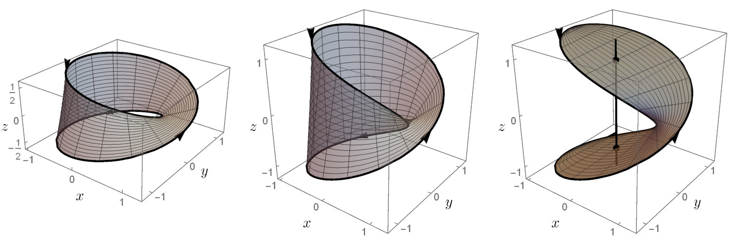 Figure 1
Peer Reviews
No public reviews on file for this paper yet. If you reviewed it on a platform where reviews are public (OpenReview, ICLR, NeurIPS, ICML), you can paste yours below so the community can read it here.
Videos
No videos yet. Explain this paper in a talk, walkthrough, or lecture? Add one.
A simple and more general approach to Stokes’ theorem
Iosif Pinelis
Michigan Technological University
**Summary ** Oftentimes, Stokes’ theorem is derived by using, more or less explicitly, the invariance of the curl of the vector field with respect to translations and rotations. However, this invariance – which is oftentimes described as the curl being a “physical” vector – does not seem quite easy to verify, especially for undergraduate students. An even bigger problem with Stokes’ theorem is to rigorously define such notions as “the boundary curve remains to the left of the surface”. Here an apparently simpler and more general approach is suggested.
In calculus texts (see e.g. [4, §XII.6] or [12, §16.8]), Stokes’ theorem is usually stated as follows: Let be an oriented smooth enough surface in bounded by a simple closed smooth enough curve with positive orientation. Then for any smooth enough vector field
[TABLE]
where is the curl of the vector field and is a continuous field of unit normal vectors on . The positive orientation of is “defined” there as the condition for the surface to remain on the left (with respect to ) when is traced out. In such elementary texts, it is of course impossible to rigorously define such notions as “remains on the left”; cf. e.g. [11, Theorems 5.5 and 5.9], [5, §XXIII.4–XXIII.6], or [2, §4.5.6]. The very concept of a surface in general is not elementary. A surface may be defined as a two-dimensional manifold-with-boundary [11] – possibly with singularities, which need to be considered to cover the case of even such simple surfaces as the (convex hulls of) triangles or rectangles; cf. e.g. [5, §XXIII]. Moreover, for the surface integral on the right-hand side of identity (1) to make sense, one has to ensure that the curl and the unit normal vector field have appropriate invariance properties with respect to the choice of an atlas for the manifold .
Green’s theorem is the special and comparatively very simple case of Stokes’ theorem corresponding to the additional condition that the surface is flat and thus may be assumed to coincide with a region . Informally, Green’s theorem may be stated as follows:
Let be a compact subset of with a smooth enough boundary , and let and be real continuously differentiable functions on an open neighborhood of . Then
[TABLE]
with the line integral appropriately defined.
One way to make this statement rigorous (and general enough) is to assume that the boundary of is a rectifiable Jordan curve oriented so as to make the winding number of equal (rather than ) with respect to any point in the interior of . These conditions on and will be assumed in the sequel.
Even though Green’s theorem is only a special case of Stokes’, it is not easy to prove the just mentioned rigorous “Jordan curve” version of it, or even to show that the winding number can be consistently defined; see e.g. [6] and references there to [9, 13, 8, 1]. The best practical approach to teaching Green’s theorem in a calculus course would probably be to restrict the consideration to simple regions, of the form or , and possibly simple combinations thereof.
Anyway, in this note we shall show that, once an appropriate version of Green’s theorem is established, it is then very easy and painless to derive versions of Stokes’ theorem, which are even more general, in some aspects, than the conventional one.
Indeed, for some open neighborhood of and , let
[TABLE]
be a twice continuously differentiable map of into . Let be the image of the boundary of under the map . Let
[TABLE]
by a continuously differentiable vector field on . Since , we can write/define the line integral as follows:
[TABLE]
Here, as usual, the subscripts u, v, denote the partial differentiation with respect to . One may say that formula (3) reduces the “line integral” over the “image-curve” (which does not have to be a simple curve, without self-intersections) to the well-defined line integral over the properly oriented rectifiable Jordan curve in the domain of the map .
Letting now and , we have
[TABLE]
since . So, Green’s theorem (2) immediately yields the following form of Stokes’ theorem:
[TABLE]
which, similarly to (1), reduces a line integral to a double one.
This may be compared with the more conventional form of Stokes’ theorem:
[TABLE]
where is a continuously differentiable 3D vector field defined on a neighborhood of the “surface”
[TABLE]
and the line integral may be understood as the one in (4) (or, equivalently, in (3)) with
[TABLE]
It is not hard to deduce (5) from (4). Indeed, let be any orthonormal basis in , in which the cross products and can be computed according to the standard determinant formulas. Let and be, respectively, the triples of the coordinates of and in the basis . Since both sides of (5) are linear in , without loss of generality , and then the integrands on the right-hand sides of (4) and (5) become, respectively,
[TABLE]
and
[TABLE]
Now it is quite easy to see that , which completes the derivation of (5) from (4).
The main distinction of (4) and (5) from (1) is that the double integrals in (4) and (5) are taken over the flat preimage-region – whereas the “image-surface” plays no role in (4) and (5), except that the vector field has to be defined on some neighborhood of . Therefore, as far as (4) and (5) are concerned, there is no need to talk about any properties of the image-surface except for it being a subset of . In particular, there is no need to talk about the orientation of or to use such hard to define terms as “remains on the left” or to care about the mentioned invariance properties of the curl and the unit normal vector field. Moreover, the image-surface , as well as the image-curve , may be self-intersecting, and does not have to be a manifold at all. As for the line integrals in (4) and (5), they are over the image-curve only in form, as they immediately reduce to line integrals over the pre-image curve , according to (3). This reduction of integration in the image-space to that in the flat preimage-space is natural; it is even unavoidable – for how else would one actually compute the line and surface integrals in the conventional form (1) of Stokes’ theorem? (Of course, to do the integration in the preimage-space, we still need a proper orientation of the boundary of the flat preimage domain , as was already pointed out in our discussion concerning a general “Jordan curve” version of Green’s theorem and its elementary version for simple regions.)
Next, let us consider (4) versus (5). We saw that (4) is very easy to obtain, modulo Green’s theorem. Arguably, (4) is also easier to remember than (5).
An important advantage of (4) is that it is more general than (5). Indeed, on the one hand, (5) follows from (4); on the other hand, in (4) the composition-factorization (6) of the map is not needed. That is, for (4) one does not need the implication (which necessarily follows from (6)).
Plus, one does not need the notion of the curl for (4). On the other hand, (4) by itself will not help when proving that a vector field is conservative if its curl is zero. Yet, as shown above, (5) is rather easy to get from (4).
We thus have three versions of Stokes’ theorem, corresponding to the three formulas:
the conventional version (1), which requires comparatively most stringent and even hard to define conditions, including an appropriate orientability of the image-surface together with the image-curve, and the invariance of the curl and the unit normal vector field;
the “computational”, less conventional version (5), which is not concerned with orientability of the images, but needs the composition-factorization condition (6);
(4), which is the most general of the three versions and, at the same time, easiest to obtain – but not useful when, say, the curl is known to be zero.
The above discussion is illustrated by
Example 1**.**
Consider the Möbius strip (of “radius” and half-width ), which is the image of the rectangle
[TABLE]
under the map given by the formula (cf. e.g. [10])
[TABLE]
The image-curve is self-intersecting, a reason being that for all one has – whereas , , and . For this reason, the “surface” may be considered self-intersecting as well. If , then is self-intersecting in another, apparently more interesting manner; cf. [7, Theorem 1.9]. Indeed, assume that and let , , , and , where is a small enough positive real number. Then – whereas , , and . Similarly, letting , , , and for small enough , we have .
Letting now, for instance, for all , we will have for all pairs of points and as above. Therefore, at the self-intersection points with and small enough , one will be unable to define a vector field so that (6) hold. Thus, formula (5) is not applicable here; of course, formula (1) is not applicable either, because the Möbius strip is not orientable.
In contrast, (4) applies with no problem in this situation; each side of (4) evaluates here to .
The problem of application of Stokes’ theorem to the Möbius strip was previously considered in [3]. The version of the Möbius strip dealt with in [3] differs by a composition of an isometry and a homothety from the apparently more common version described by (8). So, in the subsequent discussion the considerations in [3] will be translated into terms corresponding to (8). Following [3], let us introduce here the vector field defined by the formula
[TABLE]
for such that . It is noted in [3] that (i) wherever the vector field is defined and (ii) the Möbius strip does not intersect the -axis if . So, on the Möbius strip.
It is then concluded in [3] that the surface integral on the right-hand side of (1) is [math]. However, this conclusion is not quite correct, because the Möbius strip is not orientable and hence the normal vector field cannot be appropriately defined on the strip, so that the surface integral is technically not defined either and thus has no value.
Also, it is observed in [3] that the boundary (say ) of the Möbius strip is the image of the interval under the map
[TABLE]
and that the line integral over the so-parameterized curve is , which differs from the presumed value [math] of the actually undefined surface integral. This discrepancy is ascribed in [3] to the non-orientability of the Möbius strip. Now one may wonder as follows:
{quoting}
We were told in this note that, as far as (4) and (5) are concerned, there is no need to talk about the orientation of the images and of and under the map . If so, then the version (5) of Stokes’ theorem must hold even for the Möbius strip and the vector field as in (9). The double integral on the right-hand side of (5) – in contrast to that on the right-hand side of (1) – is well defined, and it must be [math], since on the Möbius strip. But the line integral over the boundary of the Möbius strip was found in [3] to be nonzero. Does this not contradict (5)?
In fact, there is no contradiction here. Recall that the line integral in (5) was to be understood as the one in (3) (with as in (6)) and, in turn, the line integral in (3) over the “image-curve” was defined as the corresponding line integral over the preimage of , where is the boundary of the preimage-region . In contrast with these conditions, the line integral in [3] was essentially taken over the segment , which is of course not the boundary of . However, the value of the line integral in (5) computed indeed as the one in (3) with as in (6) is [math], which is of course the same as the value of the double integral in (5).
At this point, one may still wonder:
{quoting}
The difficulty with the applicability of Stokes’ theorem to the Möbius strip was ascribed in [3] to the non-orientability. However, the boundary of the (non-orientable) Möbius strip can also be the boundary of an orientable surface. Then the line integral as computed in [3] will have the same value , whereas the corresponding surface integral on the right-hand side of (1) will still be [math], right? So, it seems we have another contradiction here.
The answer to this concern is as follows. First here, indeed the boundary of the Möbius strip can also be the boundary of an orientable surface. To see this, it is more convenient to use the interval instead of . More specifically, recall (8) and note that, as increases from to , the -coordinate of the vector increases from its minimal value to its maximal value ; and as increases further from to , the -coordinate of decreases from back to . Moreover, each value of the -coordinate of in the interval is taken at exactly two points and in such that . The value of the -coordinate of for is taken only at ; accordingly, assume that . Note also that decreases from to as increases from to . Connecting now, for each , the points and by (say) a straight line segment, we do obtain an orientable surface, sat , whose boundary is the same as the boundary of the Möbius strip. The surface is the image of the rectangle under the map
[TABLE]
To verify that is orientable, note that the first two coordinates of the vector are and , respectively, whence for all in the interior of , and so, one can define the unit normal vector field on the image of the interior of under the map by the formula .
Moreover and more importantly, the image under this map of the boundary of the rectangle is the boundary of the Möbius strip. So, (5) will hold for any 3D vector field which is smooth enough, in the sense of being continuously differentiable on a neighborhood of the surface . For instance, for the linear vector field defined by the formula , where is a constant real matrix and ⊤ denotes the transposition, both the left-hand side and right-hand side of (5) with (and ) take the same value, .
Is the particular field given by (9) continuously differentiable on a neighborhood of the surface ? In other words, is the intersection of the surface with the -axis empty? If that were so, then the right-hand of (5) would be [math] – whereas, as one can recheck, the value of the line integral in (5) is the same nonzero value, , as the one found the other way in [3]. It follows that the surface does intersect the -axis. In fact, it is not hard to check directly that this intersection contains exactly two points, .
A free bonus of this discussion is the fact that any orientable surface in whose boundary coincides with the boundary of the Möbius strip given by (8) must necessarily intersect the -axis. One may also note here that, for any such orientable surface and for as in (9), the surface integral on the right-hand side of (1) will actually not be [math]; rather, it will be undefined.
This discussion is partly illustrated in Fig. 1.
The reference list from the paper itself. Each links out to its DOI / PubMed record.
- 11. T. M. Apostol. Mathematical analysis: a modern approach to advanced calculus . Addison-Wesley Publishing Company, Inc., Reading, Mass., 1957.
- 22. H. Federer. Geometric measure theory . Die Grundlehren der mathematischen Wissenschaften, Band 153. Springer-Verlag New York Inc., New York, 1969.
- 33. J.-P. Gabardo. The Möbius strip and Stokes theorem, 2006. http://ms.mcmaster.ca/gabardo/moebius.pdf.
- 44. S. Lang. Calculus of Several Variables . Springer, 1987. Third ed.
- 55. S. Lang. Real and functional analysis , volume 142 of Graduate Texts in Mathematics . Springer-Verlag, New York, third edition, 1993.
- 66. Math Overflow. Proof of Green’s formula for rectifiable Jordan curves, 2018. https://mathoverflow.net/questions/307713/proof-of-greens-formula-for-rectifiable-jordan-curves.
- 77. I. Pinelis. A simpler ℝ 3 superscript ℝ 3 \mathbb{R}^{3} realization of the Möbius strip. https://arxiv.org/abs/1808.03955 , 2018.
- 88. D. H. Potts. A note on Green’s theorem. J. London Math. Soc. , 26:302–304, 1951.