Real-time Video Summarization on Commodity Hardware
Wesley Taylor, Faisal Z. Qureshi

TL;DR
This paper introduces a real-time video summarization method that operates efficiently on standard hardware, using low-level features and tree-based models to produce summaries faster than the video's duration.
Contribution
The proposed approach achieves real-time video summarization on commodity hardware with comparable accuracy to deep learning methods, but with significantly faster processing times.
Findings
Achieves real-time summarization faster than video duration
Comparable accuracy to state-of-the-art deep learning methods
Operates efficiently on standard hardware
Abstract
We present a method for creating video summaries in real-time on commodity hardware. Real-time here refers to the fact that the time required for video summarization is less than the duration of the input video. First, low-level features are use to discard undesirable frames. Next, video is divided into segments, and segment-level features are extracted for each segment. Tree-based models trained on widely available video summarization and computational aesthetics datasets are then used to rank individual segments, and top-ranked segments are selected to generate the final video summary. We evaluate the proposed method on SUMME dataset and show that our method is able to achieve summarization accuracy that is comparable to that of a current state-of-the-art deep learning method, while posting significantly faster run-times. Our method on average is able to generate a video summary in…
Click any figure to enlarge with its caption.
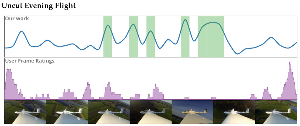 Figure 1
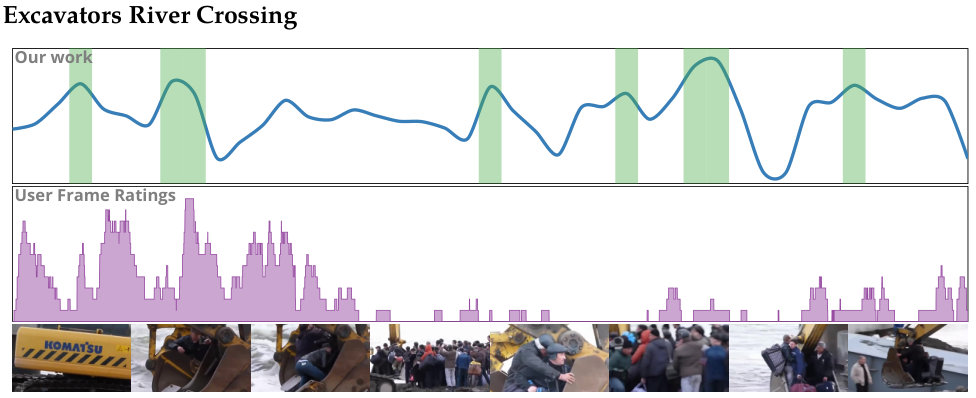 Figure 2
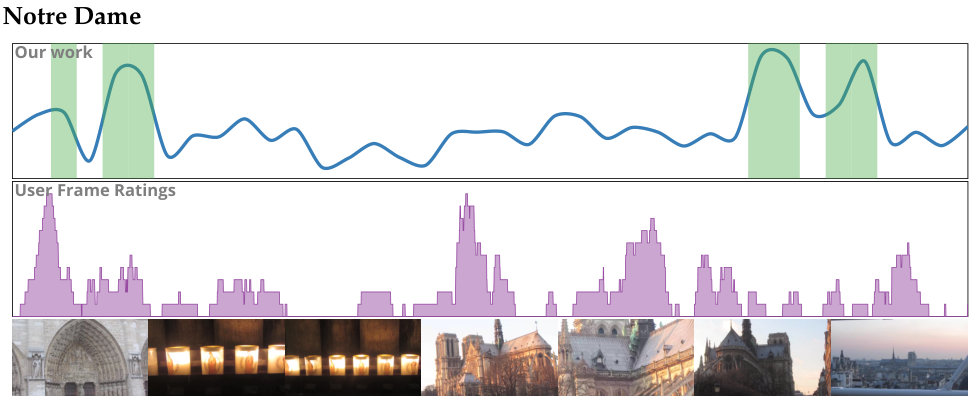 Figure 3
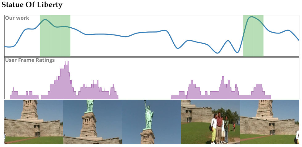 Figure 4
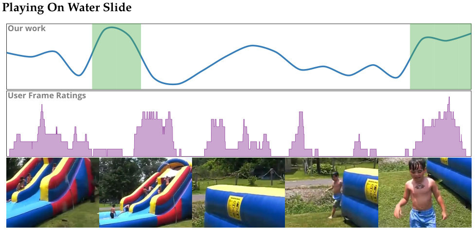 Figure 5
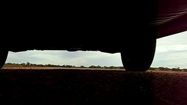 Figure 6
 Figure 7
 Figure 8
 Figure 9
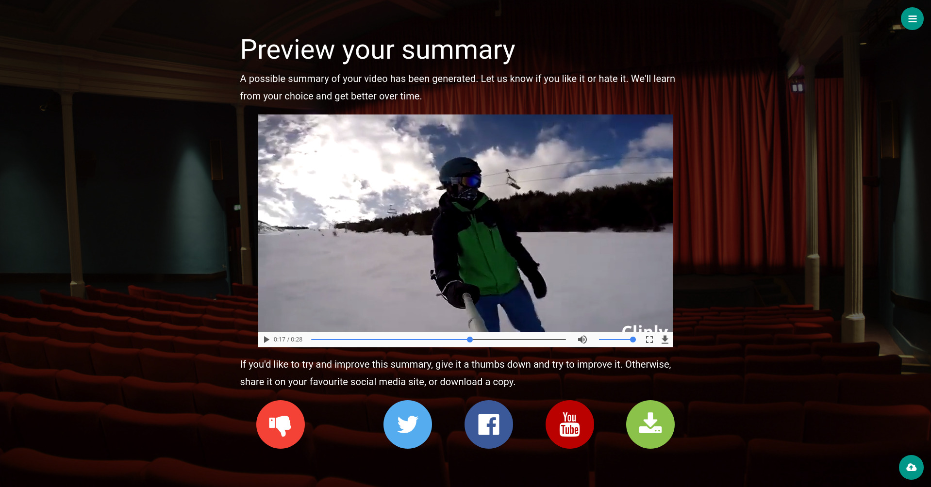 Figure 10
 Figure 11
 Figure 12
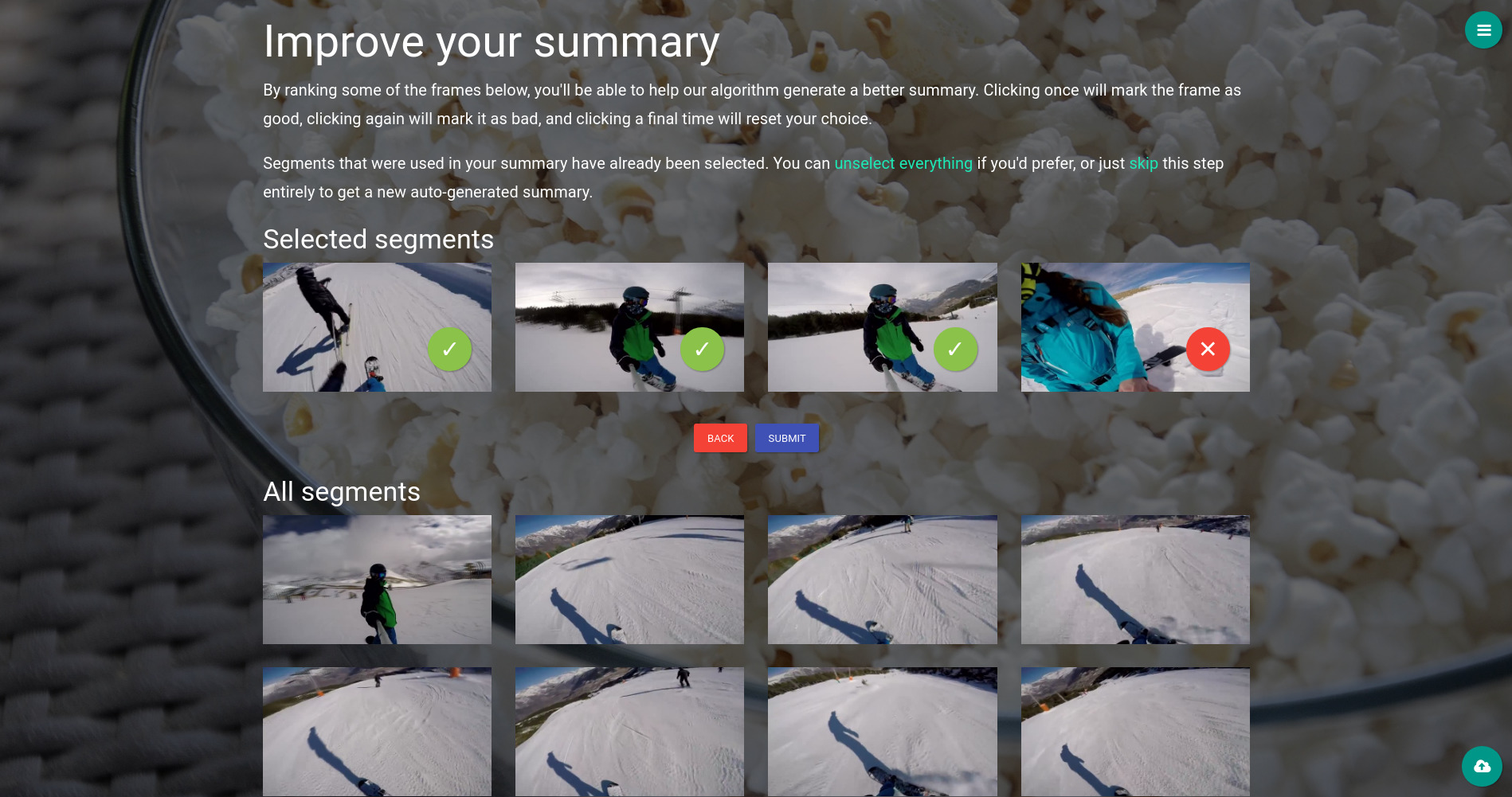 Figure 13
 Figure 14
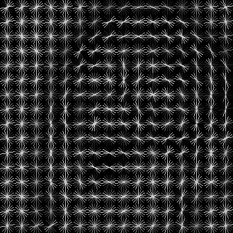 Figure 15
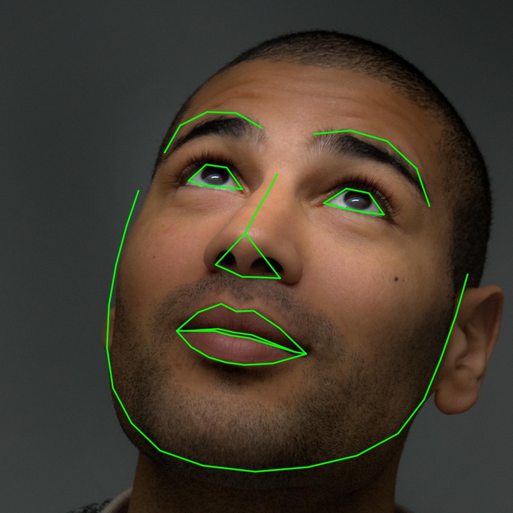 Figure 16
 Figure 17
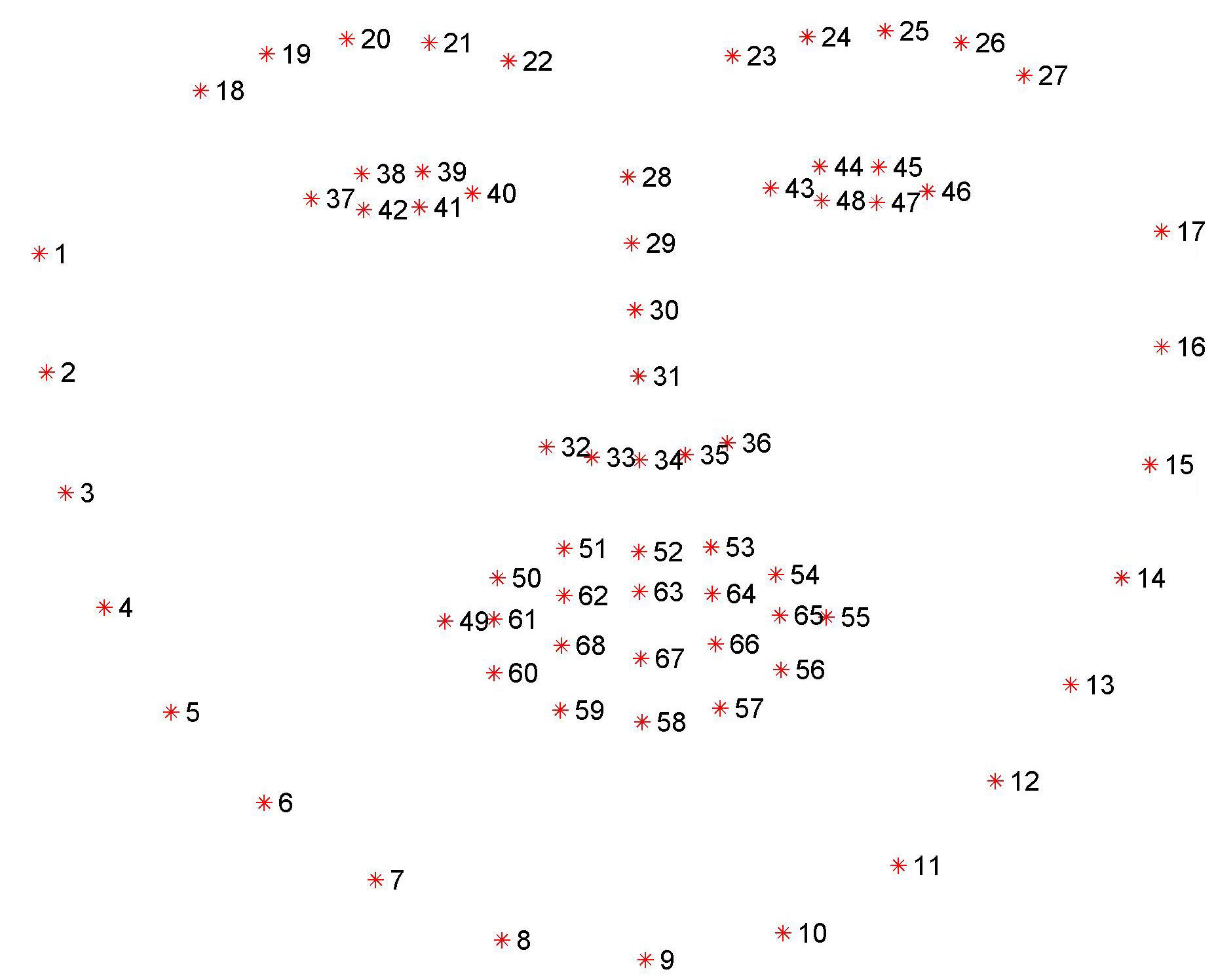 Figure 18
 Figure 19
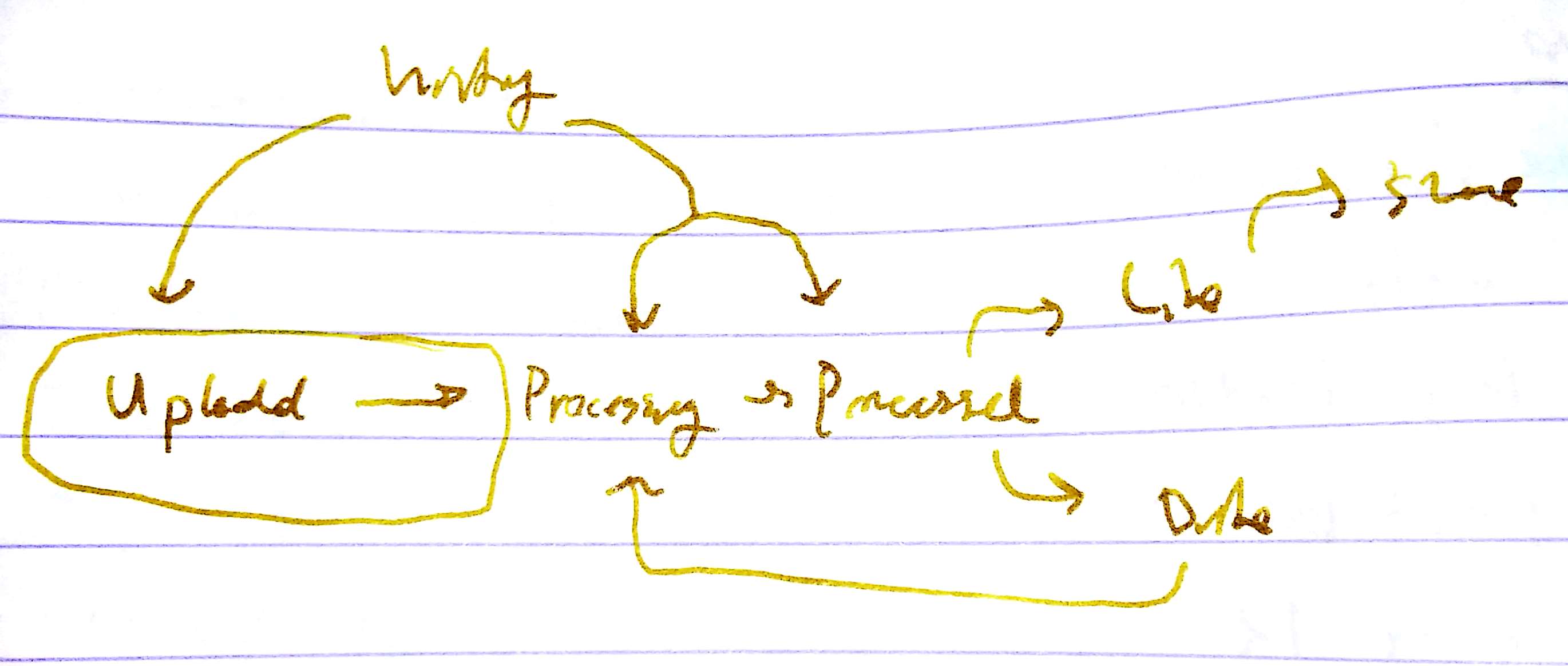 Figure 20
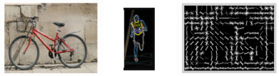 Figure 21
 Figure 22
 Figure 23
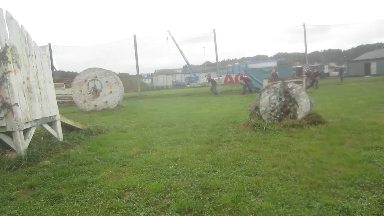 Figure 24
 Figure 25
| Feature | Dim. | Description |
| Contrast | 1 | The ratio between the luminance range and average luminance. |
| Image Mean HSV | 3 | The average H, S, and V values over the entire image. |
| Center Mean HSV | 3 | The average H, S, and V values for the image center quadrant. |
| Itten Histograms (Machajdik and Hanbury, 2010) | 20 | Histograms of H values over 12 bins, S values over 5 bins, and V values over 3 bins. |
| Itten Contrasts (Machajdik and Hanbury, 2010) | 3 | Standard deviation of each Itten Histogram. |
| Pleasure, Arousal, Dominance (Machajdik and Hanbury, 2010) | 3 | Approximate emotional values computed as linear combinations of the mean V and S values. |
| Haralick Texture Features (Haralick et al., 1973) | 13 | Average Haralick texture features over all four directions. |
| Contrast Balance | 1 | Distance between the original and contrast-normalized grayscale image. |
| Exposure Quality | 1 | Negative absolute value of luminance histogram skew. |
| JPEG Quality (Sheikh et al., 2002) | 1 | No-reference quality estimation algorithm for JPEG images. |
| Tenengrad (Ng et al., 2001) | 1 | Sharpness according to the Tenengrad method. |
| Spectral Residual (Hou and Zhang, 2007) | 9 | Rule of thirds using spectral saliency in 9 quadrants. |
| Model | Min | Max | Mean | Std. Dev. |
| Decision Tree | ||||
| Random Forest | ||||
| XGBoost |
| Dataset | Humans | Computational Methods | ||||||||
| Videoname | Random | Upper Bound | Worst | Mean | Best | Uniform | Cluster | Attn. | Summe | Ours |
| Air Force One | 0.144 | 0.490 | 0.185 | 0.332 | 0.457 | 0.161 | 0.143 | 0.215 | 0.318 | 0.362 |
| Base jumping | 0.144 | 0.398 | 0.113 | 0.257 | 0.396 | 0.168 | 0.109 | 0.194 | 0.121 | 0.106 |
| Bearpark climbing | 0.147 | 0.330 | 0.129 | 0.208 | 0.267 | 0.152 | 0.158 | 0.227 | 0.118 | 0.261 |
| Bike Polo | 0.134 | 0.503 | 0.190 | 0.322 | 0.436 | 0.058 | 0.130 | 0.076 | 0.356 | 0.301 |
| Bus in Rock Tunnel | 0.135 | 0.359 | 0.126 | 0.198 | 0.270 | 0.124 | 0.102 | 0.112 | 0.135 | 0.147 |
| Car railcrossing | 0.140 | 0.515 | 0.245 | 0.357 | 0.454 | 0.146 | 0.146 | 0.064 | 0.362 | 0.192 |
| Cockpit Landing | 0.136 | 0.443 | 0.110 | 0.279 | 0.366 | 0.129 | 0.156 | 0.116 | 0.172 | 0.201 |
| Cooking | 0.145 | 0.528 | 0.273 | 0.379 | 0.496 | 0.171 | 0.139 | 0.118 | 0.321 | 0.348 |
| Eiffel Tower | 0.130 | 0.467 | 0.233 | 0.312 | 0.426 | 0.166 | 0.179 | 0.136 | 0.295 | 0.088 |
| Excavators river crossing | 0.144 | 0.411 | 0.108 | 0.303 | 0.397 | 0.131 | 0.163 | 0.041 | 0.189 | 0.231 |
| Fire Domino | 0.145 | 0.514 | 0.170 | 0.394 | 0.517 | 0.233 | 0.349 | 0.252 | 0.130 | 0.169 |
| Jumps | 0.149 | 0.611 | 0.214 | 0.483 | 0.569 | 0.052 | 0.298 | 0.243 | 0.427 | 0.542 |
| Kids playing in leaves | 0.139 | 0.394 | 0.141 | 0.289 | 0.416 | 0.209 | 0.165 | 0.084 | 0.089 | 0.093 |
| Notre Dame | 0.137 | 0.360 | 0.179 | 0.231 | 0.287 | 0.124 | 0.141 | 0.138 | 0.235 | 0.107 |
| Paintball | 0.127 | 0.550 | 0.145 | 0.399 | 0.503 | 0.109 | 0.198 | 0.281 | 0.320 | 0.213 |
| Playing on water slide | 0.134 | 0.340 | 0.139 | 0.195 | 0.284 | 0.186 | 0.141 | 0.124 | 0.200 | 0.218 |
| Saving dolphines | 0.144 | 0.313 | 0.095 | 0.188 | 0.242 | 0.165 | 0.214 | 0.154 | 0.145 | 0.128 |
| Scuba | 0.138 | 0.387 | 0.109 | 0.217 | 0.302 | 0.162 | 0.135 | 0.200 | 0.184 | 0.140 |
| St Maarten Landing | 0.143 | 0.624 | 0.365 | 0.496 | 0.606 | 0.092 | 0.096 | 0.419 | 0.313 | 0.557 |
| Statue of Liberty | 0.122 | 0.332 | 0.096 | 0.184 | 0.280 | 0.143 | 0.125 | 0.083 | 0.192 | 0.259 |
| Uncut Evening Flight | 0.131 | 0.506 | 0.206 | 0.350 | 0.421 | 0.122 | 0.098 | 0.299 | 0.271 | 0.081 |
| Valparaiso Downhill | 0.142 | 0.427 | 0.148 | 0.272 | 0.400 | 0.154 | 0.154 | 0.231 | 0.242 | 0.288 |
| car over camera | 0.134 | 0.490 | 0.214 | 0.346 | 0.418 | 0.099 | 0.296 | 0.201 | 0.372 | 0.408 |
| paluma jump | 0.139 | 0.662 | 0.346 | 0.509 | 0.642 | 0.132 | 0.072 | 0.028 | 0.181 | 0.334 |
| playing ball | 0.145 | 0.403 | 0.190 | 0.271 | 0.364 | 0.179 | 0.176 | 0.140 | 0.174 | 0.151 |
| Average | 0.139 | 0.454 | 0.179 | 0.311 | 0.409 | 0.143 | 0.163 | 0.167 | 0.234 | 0.237 |
| Video Name | Duration (s) | Time (s) | Speed |
| Jumps | 38.00 | 19.12 | 1.99x |
| Cooking | 85.80 | 22.16 | 3.87x |
| Fire Domino | 53.73 | 27.99 | 1.92x |
| St Maarten Landing | 70.04 | 36.72 | 1.91x |
| Scuba | 74.03 | 48.45 | 1.53x |
| paluma jump | 85.89 | 46.89 | 1.83x |
| Bike Polo | 102.13 | 69.50 | 1.47x |
| Playing on water slide | 102.27 | 54.76 | 1.87x |
| playing ball | 103.97 | 54.52 | 1.91x |
| Kids playing in leaves | 106.34 | 71.29 | 1.49x |
| Bearpark climbing | 133.64 | 78.31 | 1.71x |
| Statue of Liberty | 154.52 | 69.89 | 2.21x |
| car over camera | 146.21 | 71.04 | 2.06x |
| Air Force One | 179.76 | 103.59 | 1.74x |
| Notre Dame | 192.00 | 106.87 | 1.80x |
| Base jumping | 157.79 | 105.27 | 1.50x |
| Eiffel Tower | 198.84 | 118.90 | 1.67x |
| Car railcrossing | 169.34 | 115.14 | 1.47x |
| Bus in Rock Tunnel | 171.10 | 109.00 | 1.57x |
| Valparaiso Downhill | 172.77 | 115.51 | 1.50x |
| Paintball | 254.25 | 137.37 | 1.85x |
| Saving dolphines | 222.99 | 120.15 | 1.86x |
| Cockpit Landing | 301.83 | 200.50 | 1.51x |
| Uncut Evening Flight | 322.72 | 215.42 | 1.50x |
| Excavators river crossing | 388.84 | 210.87 | 1.84x |
| Average | 1.82x |
Peer Reviews
No public reviews on file for this paper yet. If you reviewed it on a platform where reviews are public (OpenReview, ICLR, NeurIPS, ICML), you can paste yours below so the community can read it here.
Videos
No videos yet. Explain this paper in a talk, walkthrough, or lecture? Add one.
\DeclareAcronym
LASSO short=LASSO, long=least absolute shrinkage and selection operator
\DeclareAcronymAVA short=AVA, long=A Large-Scale Database for Aesthetic Visual Analysis, pdfstring=A Large-Scale Database for Aesthetic Visual Analysis (AVA)
\DeclareAcronymCART short=CART, long=Classification And Regression Trees
\DeclareAcronymHOG short=HOG, long=Classification And Regression Trees
\DeclareAcronymFHOG short=FHOG, long=Felzenszwalb’s HOG
\DeclareAcronymLFW short=LFW, long=Labeled Faces in the Wild
\DeclareAcronymSUMME short=SumMe, long=The SumMe Video Summarization
\DeclareAcronymTVSUM50 short=TVSum50, long=Summarizing Web Videos using Titles
\AtBeginShipoutNext\AtBeginShipoutDiscard
Real-time Video Summarization on Commodity Hardware
Wesley Taylor and Faisal Z. Qureshi
Faculty of Science, University of Ontario Institute of TechnologyUA4000, 2000 Simcoe St. N.OshawaON L1G 0C5 Canada
wesley.taylor3—[email protected]
(2018; 2018)
Abstract.
We present a method for creating video summaries in real-time on commodity hardware. Real-time here refers to the fact that the time required for video summarization is less than the duration of the input video. First, low-level features are use to discard undesirable frames. Next, video is divided into segments, and segment-level features are extracted for each segment. Tree-based models trained on widely available video summarization and computational aesthetics datasets are then used to rank individual segments, and top-ranked segments are selected to generate the final video summary. We evaluate the proposed method on \acSUMME dataset and show that our method is able to achieve summarization accuracy that is comparable to that of a current state-of-the-art deep learning method, while posting significantly faster run-times. Our method on average is able to generate a video summary in time that is shorter than the duration of the video.
Video summarization, video analysis
††copyright: rightsretained††doi: 10.475/123_4††isbn: 123-4567-24-567/08/06††conference: ACM International Conference on Distributed Smart Cameras; September 2018; Eindhoven, Netherlands††journalyear: 2018††article: 4††price: 15.00††journalyear: 2018††copyright: acmcopyright††conference: International Conference on Distributed Smart Cameras; September 3–4, 2018; Eindhoven, Netherlands††booktitle: International Conference on Distributed Smart Cameras (ICDSC ’18), September 3–4, 2018, Eindhoven, Netherlands††price: 15.00††doi: 10.1145/3243394.3243689††isbn: 978-1-4503-6511-6/18/09††ccs: Computing methodologies Video summarization
1. Introduction
Cameras are now ubiquitous. This has resulted in an explosive growth in user-generated images and videos. In the case of videos, at least, our ability to record videos has far outpaced methods and tools to manage these videos. A skier, for example, can easily record many hours of video footage using an action camera, such as a GoPro. Raw video footage, in general, is unviewable—the recorded video needs to be summarized or edited in some manner before it can be shared with others. Clearly, no one is interested in watching many hours of skiing video when most of it is bound to be highly repetitive. Manual video editing and summarizing is painstakingly slow and tedious. Consequently a large fraction of recorded footage is never shared or even viewed. We desperately need one-touch video editing tools capable of generating video summarizes that capture the meaningful and interesting portions of the video, discarding sections that are boring, repetitive or poorly recorded. Such tools will revolutionize how we share video stories with friends and family via social media.
A meaningful video summarization needs to take into account both the user context and the video content. Two different users may find entirely different sections of a recorded video interesting. Consider, for example, the scenario where someone records a children soccer match. Parents may only be interested in a section in video that shows their child. We refer to this as user context. Video summarization algorithms, therefore, should take into account the likes and dislikes of the viewers of the video summary. Video content is also important. By necessity video summarization algorithms relies upon video content to select which portions of the videos make the cut.
This paper develops a real-time video summarization system (Figure 1). The proposed system is able to perform video summarization at speeds that far exceed those achieved by state-of-the-art deep learning approaches for video summarization. We list these approaches in the next section. The proposed system exploits low-level image features to efficiently discard segments with low interestingness or having poor quality. This means that subsequent summarization steps, which are computationally expensive, only deal with the remaining segments. This can lead to significant savings, especially for long duration videos, such as the all day ski trip video in the example mentioned above. A key feature of the proposed system is its ability to generate alternate summaries almost instantaneously. A user can guide the system to generate a different summary thereby injecting user-preference into the process of summarization. Figure 1 shows our summarization pipeline.
We evaluate the proposed method on SumMe video summarization benchmark, and compare our method with a number of existing video summarization schemes. Our method achieves the highest -measure. It also achieves highest accuracy on over 50% of the tested videos. We also show that the summarization times of the proposed method increases linearly with the duration of the input video.
The rest of the paper is organized as follows. We briefly discuss related work in the next section. Section 3 discusses video segmentation. Segment ranking is covered in Section 4. The following section describes video summarization. We conclude the paper with evaluation and results and conclusions in the last two sections.
2. Background
A majority of the existing video summarization methods follow a common recipe: step 1) video segmentation, step 2) segment ranking and step 3) segment selection (Lee et al., 2012; Ejaz et al., 2013; Gygli et al., 2014; Song et al., 2016). Methods vary in how segmentation is performed and how individual segments are ranked. (Zhang et al., 2016) is an exception to this rule that uses recent advances in deep learning and provides an end-to-end system for video summarization. This method relies upon the availability of suitable training data. Early video summarization methods were unsupervised (Lee et al., 2012; Ejaz et al., 2013; Song et al., 2016); however, with the recent availability of high-quality video summarization datasets, many newer methods are supervised (Gygli et al., 2014; Zhang et al., 2016).
Video summarization has also been explored in the context of robotics (Girdhar, 2014). Their motivation stems from the fact that transmitting raw video footage, say to a base station, incurs large communication costs. It is also infeasible in situations where bandwidth is limited. They leverage topic modeling to identify the novel segments of the recorded video with a view to construct a video summarization that captures the salient pieces of the video.
Clustering (Lee et al., 2012) and attention (Ejaz et al., 2013) methods are often used as baselines when evaluating new summarization methods. The first method performs clustering to get segmentation, and uses a 0/1 knapsack for segment selection for final summary generation. The second method extracts attention features for each frame, assigning an interestingness score to each frame. Frames with high interestingness scores are selected to generate the summary. We refer the kind reader to the respective publications for technical details. Suffice to say that both classes of methods are unsupervised and are able to achieve higher accuracy when compared to a method that picks frames (or segments) at random when generating a video summarization. Recent methods outperform both these methods.
Method developed in (Gygli et al., 2014) is of particular interest to us. (Gygli et al., 2014) not only developed a new method for video summarization. It also created a first-of-its-kind benchmark for video summarization. This dataset is referred to as the SumMe dataset. We too use this dataset to evaluate the performance of our method. (Gygli et al., 2014) uses change point detection for segmentation. These segments are subsequently ranked and the final summary is generated using a 0/1 knapsack formulation. (Song et al., 2016) method is similar to the method proposed in (Gygli et al., 2014). The key difference is that (Song et al., 2016) method uses a different set of features for ranking segments.
The current best performing video summarization method is (Zhang et al., 2016). It uses convolutional and recurrant layers that operate upon sequences of frames and compute interestingness score for each frame. Specifically, this method uses pool-5 layer of GoogLeNet model as frame-level features, which are fed into LSTM units to generate frame and segment level interestingness scores. The key idea is to capture temporal relationship between successive frames to compute frame-level interestingness score suitable for video summarization.
3. Video Segmentation
The algorithm begins by identifying frames that are too dark, blurry, or uniform (see Figure 2). Luminance (), sharpness () and uniformity () values are computed for each frame to label the frame accordingly. Luminance is given by
[TABLE]
sharpness is computed as
[TABLE]
uniformity value is computed by first constucting a normalized 1D grayscale histgoram with 128 bins and then computing the ratio between the top percentile bins of and the rest of . These features have low computational overhead. The algorithm thus avoids wasting precious computational resources (during the subsequent steps) on frames that will not make the final cut any ways.
Next, input video is divided into one or more non-overlapping segments
[TABLE]
While these segments do not overlap, we allow for gaps between adjacent segments, i.e., we only require that . We formulate our video as a multidimensional time-series, allowing us to cast video segmentation as a multiple change point detection problem (Bleakley and Vert, 2011; Song et al., 2015).
Change point detection operates upon a time series feature matrix , where column stores features extracted from frame . Our method extracts -dimensional feature vector from each video frame. Specifically each frame is represented using a HSV histogram with 128 bins per channel and an edge orientation and magnitude histogram with 30 bins each. These features are extracted over a two-level pyramid consisting of 5 regions, which yields a -dimensional feature. Each video is now represented as a matrix . Here indicates the number of frames. A set of sparse coefficients is computed from by solving the following convex optimization problem.
[TABLE]
is used to assign a score to each frame, and the top ranked frames are selected as split points to generate segments. We set the problem so that average segment duration is roughly seconds. This method can be thought of as a more robust version of threshold-based and content-aware sampling. Rather than relying simply on local color or brightness features, a combination of color and edge histograms are used to locate segment boundaries based on the statistical properties of the entire video.
Next we refine the segmentation by removing dark, blurry or uniform frames. Segments having a large fraction of undesirable frames are discarded in the process, which also results in further savings down the line. Segments can also be trimmed, discarding undesirable frames at the either end, or split into two or more segments. Adjacent segments containing too few frames are also merged to form a single segment at this stage. This process is shown in Algorithm 1.
4. Segment Ranking
Once all candidate segments for our video have been located, the next step is to rank these segments. The algorithm begins by extracting frame-wise features, which are subsequently used to rank the individual segments.
4.1. Frame-Level Features
We compute a 62 dimensional feature vector for each frame as follows. The first 59 dimensions correspond to computational aesthetic features computed at each frame (Table 1). We refer the interested reader to (Schifanella et al., 2015; Redi et al., 2015; Machajdik and Hanbury, 2010; Zhou et al., 2016) for technical details about these features. Dimensions 60 contains the number of faces seen in this frame, and dimension 61 records the number of “salient” faces seen in this frame. The last dimension stores a 1 if the frame is deemed aesthetically pleasing (see below).
4.1.1. Salient Face Detection
The process of finding salient faces consists of three steps: a) face detection, b) (face) feature vector extraction, and c) (face) clustering. The algorithm employs \acFHOG for face detection (Forsyth, 2014). To extract a face feature vector, we employ a modfied version of ResNet-34 (He et al., 2016), containing only 29 layers and half the number of filters in each layer. We train the network using a metric loss function over 3 million faces from the FaceScrub (Ng and Winkler, 2014) and VGG-Face (Parkhi et al., 2015) datasets. This model is able to predict with accuracy if two faces belong to the same individual on the \acLFW (Learned-Miller et al., 2016) dataset.
Face feature vectors are clustered using Chinese whispers graph clustering algorithm (Biemann, 2006). Chinese whispers is a linear-time hard partitioning, randomized, flat clustering method. A linear-time algorithm is highly desirable since an hour long video can easily contain more than 50,000 face feature vectors. Clustering ensures that each “person” ends up in at most one cluster. Clusters with large memberships identify salient persons. Note that this method requires no prior knowledge about salient faces.
The initial “graph” used as input to the clustering algorithm is constructed by simply looping over every pair of features
[TABLE]
across all segments and frames computed in the previous step, and creating an “edge” between two nodes when their distance is below some threshold value . A value of was selected, as it matches the value that was used for the metric loss layer of the deep neural network used in the previous step.
4.1.2. Aesthetic Score
The last dimension contains an aesthetic score of 0 or 1 for this frame. We use an XGBoost classifier trained on \acAVA (Murray et al., 2012) dataset to compute this score. Each image in \acAVA dataset has an associated user score between 0 and 1, which captures the aesthetic appeal of that image. For our purposes, we assign a score of 0 for any image with ranking less than 0.5. Images with ranking more than 0.5 are assigned a score of 1. We train an XBGoost classifier using 10-fold cross-validation and a train/test split of . The input to this classifier are computational aesthetic features listed in Table 1. The XGBoost classifier obtains an accuracy of , which is significantly higher than the reference model shown in (Murray et al., 2012). The accuracy of reference model is . ILGnet (Jin et al., 2016) posts the current best accuracy of . ILGnet is a deep learning based model, which is more tricky to train and has significantly worse runtime performance than our XGBoost classifier.
4.2. Segment Features
The proposed method computes segment-level features by aggregating frame-level features extracted from frames belonging to each segment. Recall that each frame is represented as a 62 dimensional feature . Segment-level feature for each segment is
[TABLE]
4.3. Ranking
We studied three models—(1) decision trees, (2) random forests, and (3) XGBoost—for ranking segments using the segment features discussed in the previous section. We trained interestingness prediction models for each of the above using segment-level features extracted from videos available in \acSUMME and \acTVSUM50 datasets. For training purposes these videos are divided into 5 second segments, and segment-level features are extracted for each segment. Train-test splits are generated using 10-fold cross-validation on shuffled data, and the mean-squared-error is used as the error metric for evaluating each model. The results for each model are presented in Table 2.
As we can see from Table 2, both the XGBoost and random forest models obtain very similar error rates, with XGBoost slightly out-performing the random forest model, and both significantly out-performing the decision tree model. For this reason, we will use both XGBoost and random forest models for evaluating our system.
4.4. Feature Importance
It is straightforward to compute feature importance when using Decision Trees and XGBoost. In order to see the efficacy of our choice of features, we performed feature importance analysis. Feature importance values are normalized between 0 and 1. A value of 1 suggests that this feature plays an important role within the model. Similarly, a value of 0 indicates that this feature is rarely used during the prediction task. Figure 3 plots feature importance for XGBoost model.
One important conclusion we can draw from Figure 3 is that among all the features used by our model, face detection and recognition features have the least average importance. These features, incidently, are computationally expensive to compute. Our initial hypothesis was that the computational cost of these features would be offset by their actual importance when computing a segment ranking. Figure 3 shows that this is obviously not the case. We, therefore, decided to exclude face detection and recognition features during segment ranking. This leaves a 120 dimensional feature for segment ranking: .
Figure 3 suggests that features constructed using XGBoost predictions have the highest average importance score. Recall that XGBoost model is trained on \acAVA dataset. This means that we are able to train a supervised model for individual image aesthetics and successfully apply this model to the task of segment ranking within the context of video summarization.
5. Video Summarization
The final summary leverages segment rankings computed previously. We formulate segment selection as a 0/1 knapsack problem. Given a set of items (segments) , each with a weight (duration) and a value (ranking) , we determine which segments to include in our final summary such that the final length is less than or equal to our target summary duration, and the sum of segment rankings is maximized. Mathematically, we can describe this as
[TABLE]
This can be solved via dynamic programming (Vance, 1993). Define as an array, and as the maximum score that can be obtained with duration up to or less than using the first items of . We get the following recursive definition:
[TABLE]
The solution can be found by computing the value of .
6. Evaluation and Results
We evaluate the proposed method using pairwise F-measure on \acSUMME dataset. \acSUMME contains multiple summaries from different users, and we need a mechanism for comparing the summary generated by our method with these user-generated summaries. (Gygli et al., 2014) proposed pairwise F-measure to perform this comparison and evaluate the performance of a summarization scheme. F-measure is computed as follows. Given a summary and a set of a set of user-generated summaries , for each in compute
[TABLE]
and
[TABLE]
Pairwise F-measure is then
[TABLE]
For the Random Forest and XGBoost models from Section 4.3, we perform grid search over various model parameters, and continue with the optimal parameters for each variable. In the end, we compare the final pairwise F-measure measures between the Random Forest and XGBoost models, and select the model which attains the highest value. Better methods are represented by higher F-measure values.
Using the default parameters for our XGBoost model, our method obtains an average F-measure value of . Average F-measure scores obtained by competing methods in (Gygli et al., 2014) and (Song et al., 2015) on \acSUMME dataset are and , respectively. We fine-tuned the XGBoost model for segment ranking. The following parameters were considered during grid search: max depth, minimum child weight, gamma, subsample and col-sample by-tree. For our dataset, the optimal values for max depth, minimum child weight, gamma, subsample and col-sample-by-tree are , , [math], and , respectively. F-measure was improved from to using these values.
6.1. Accuracy on \acSUMME Dataset
We now compare our model to existing techniques on \acSUMME dataset. Table 3 lists accuracy values for various methods on \acSUMME dataset. Our method achieves the highest average F-measure among the 5 computational video summarization schemes listed here. Average F-measure scores are provided for different videos in the \acSUMME dataset. Our method posts the highest scores for roughly 50% of the tested videos.
6.2. Performance
We performed video summarization for each video in the \acSUMME dataset using our method and recorded the times needed to generate the summaries. These times are shown in Table 4. Notice that summarization times are smaller than the duration of the videos. The third column shows the speed of video summarization process. On average our method achieves a speed of times the actual duration of the video. In other words the time it takes to summarize a video is on average times the duration of the video. Figure 4 plots summarization times vs. video durations. It suggests a linear relationship between summarization times and video durations. We fit a first-degree polynomial to this data. The coefficient of determination for this fit is , suggesting that a line is a good estimator for this data.
Figure 5 plots average performance vs. accuracy for different methods. A performance value of 1.0 indicates that the summerization time is the same as the duration of the video. We desire methods with performance greater than 1.0. We can view these methods as faster than real-time. Newer, computationally expensive methods—SumMe and LSTM—achieve high summarization accuracy; however, these methods posts poor performance. Older, simpler methods on the other hand show high performance scores. These methods, however, have low accuracy scores. Our method is able to achieve high scores for both performance and accuracy. Only the LSTM method is able to achieve a higher accuracy score than our method; however, the LSTM method has significantly lower average performance than our method. Figure 6 shows summarization results for our method on a selection of videos taken from the \acSUMME dataset.
7. Conclusions
We propose a high performance video summarization system which is able to perform video summarization in an online fashion on commodity hardware. The results demonstrate that our method is able to acquire comparable summarization quality at a fraction of a computational costs of a state-of-the-art LSTM method. Our method, for example, is able to create video summaries of arbitrary duration on a commodity desktop—a i5-3380M CPU and with 16GB of RAM and no dedicated GPU—at times less than the duration of the videos. This suggests that our method may be ideally suited for mobile deployment.
The primary limitation of our method stems from how features are computed for each segment. We have chosen low-level features, which are computationally inexpensive to extract. A downside is that these features are fundamentally limited in terms of capturing semantic information present in a video. We aim to solve this shortcoming in the future by incorporating additional features into our framework. We are also investigating methods to adapt our framework to incorporate user preferences when creating video summaries.
The reference list from the paper itself. Each links out to its DOI / PubMed record.
- 1(1)
- 2Biemann (2006) Chris Biemann. 2006. Chinese Whispers. In Proc. Text Graphs: the First Workshop on Graph Based Methods for Natural Language Processing . Association for Computational Linguistics. https://doi.org/10.3115/1654758.1654774 · doi ↗
- 3Bleakley and Vert (2011) Kevin Bleakley and Jean-Philippe Vert. 2011. The Group Fused Lasso for Multiple Change-Point Detection. ar Xiv preprint ar Xiv:1106.4199 (2011).
- 4Ejaz et al . (2013) Naveed Ejaz, Irfan Mehmood, and Sung Wook Baik. 2013. Efficient Visual Attention Based Framework for Extracting Key Frames from Videos. Sig. Proc.: Image Comm. 28, 1 (2013), 34–44. https://doi.org/10.1016/j.image.2012.10.002 · doi ↗
- 5Forsyth (2014) David A. Forsyth. 2014. Object Detection with Discriminatively Trained Part-Based Models. IEEE Computer 47, 2 (2014), 6–7. https://doi.org/10.1109/MC.2014.42 · doi ↗
- 6Girdhar (2014) Yogesh Girdhar. 2014. Unsupervised Semantic Perception, Summarization, and Autonomous Exploration for Robots in Unstructured Environments . Ph.D. Dissertation. Mc Gill University.
- 7Gygli et al . (2014) Michael Gygli, Helmut Grabner, Hayko Riemenschneider, and Luc J. Van Gool. 2014. Creating Summaries from User Videos. In Proc. 13th European Conf. on Computer Vision (ECCV 2014), Zurich, Switzerland, September 6-12, 2014, Part VII (Lecture Notes in Computer Science) , David J. Fleet, Tomás Pajdla, Bernt Schiele, and Tinne Tuytelaars (Eds.), Vol. 8695. Springer, 505–520. https://doi.org/10.1007/978-3-319-10584-0 · doi ↗
- 8Haralick et al . (1973) Robert M. Haralick, K. Sam Shanmugam, and Its’hak Dinstein. 1973. Textural Features for Image Classification. IEEE Trans. Systems, Man, and Cybernetics 3, 6 (1973), 610–621. https://doi.org/10.1109/TSMC.1973.4309314 · doi ↗