Clustering Discrete-Valued Time Series
Tyler Roick, Dimitris Karlis, Paul D. McNicholas

TL;DR
This paper develops a clustering approach for discrete-valued time series using INAR models within a finite mixture framework, enabling effective clustering and model selection.
Contribution
It introduces a novel combination of INAR models with finite mixture models for clustering discrete-valued time series data.
Findings
Effective clustering demonstrated on real data
Model selection and estimation via EM algorithm
Applicable to various discrete time series datasets
Abstract
There is a need for the development of models that are able to account for discreteness in data, along with its time series properties and correlation. Our focus falls on INteger-valued AutoRegressive (INAR) type models. The INAR type models can be used in conjunction with existing model-based clustering techniques to cluster discrete-valued time series data. With the use of a finite mixture model, several existing techniques such as the selection of the number of clusters, estimation using expectation-maximization and model selection are applicable. The proposed model is then demonstrated on real data to illustrate its clustering applications.
Click any figure to enlarge with its caption.
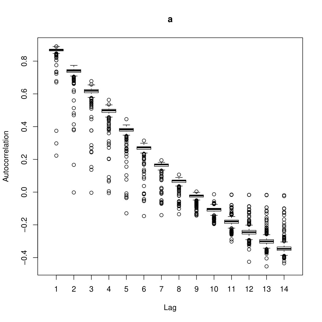 Figure 1
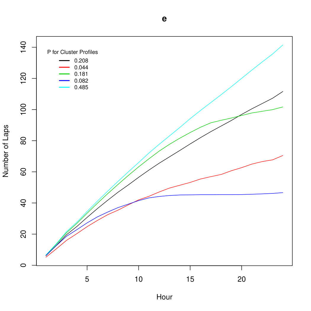 Figure 2
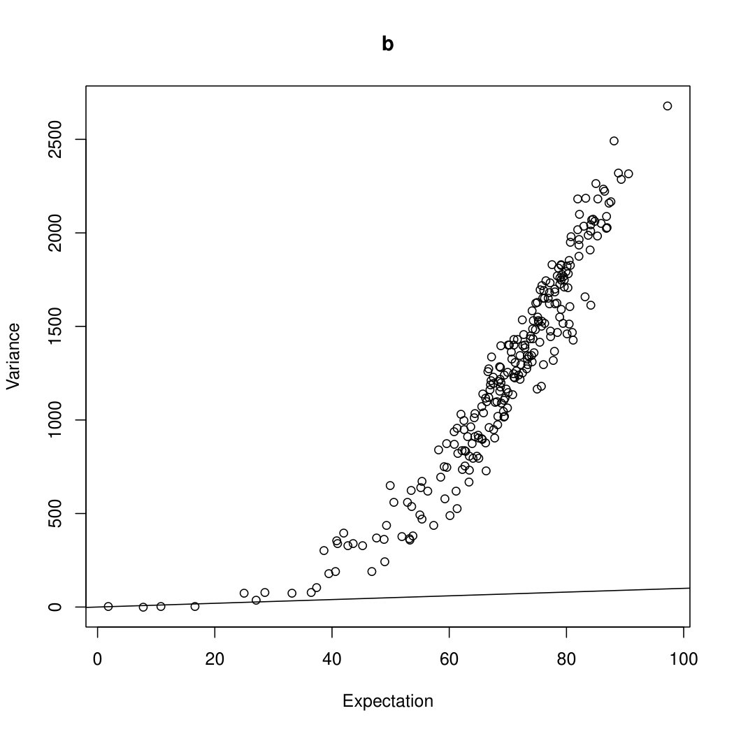 Figure 3
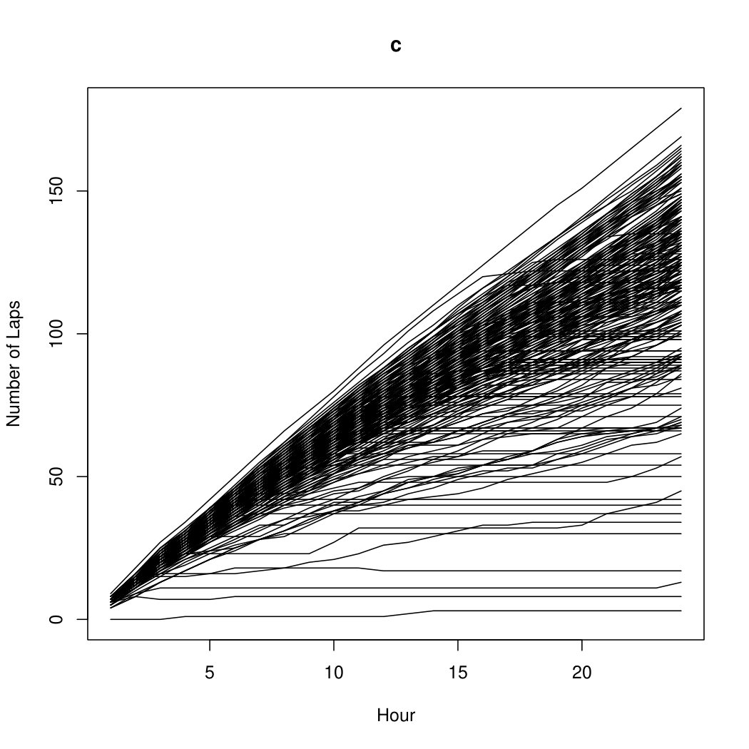 Figure 4
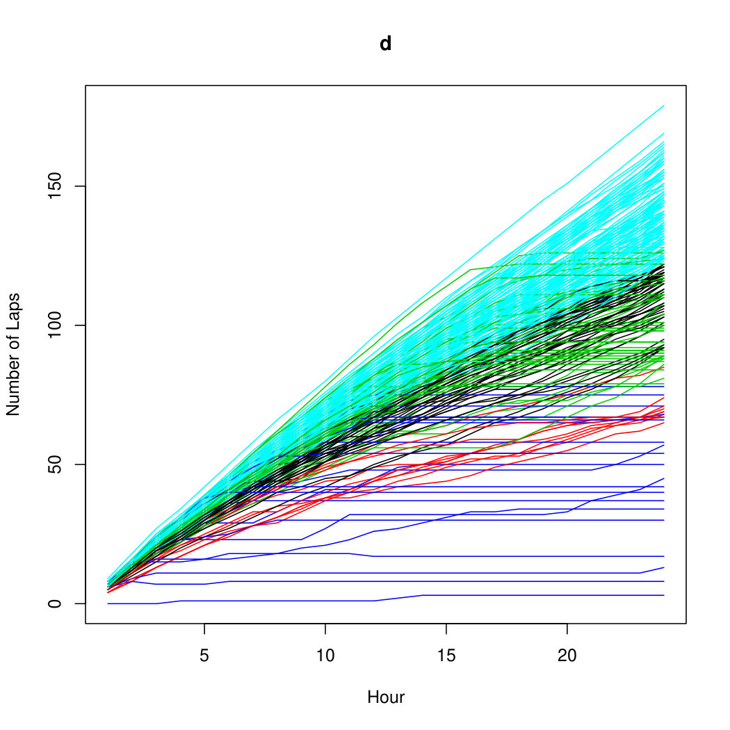 Figure 5
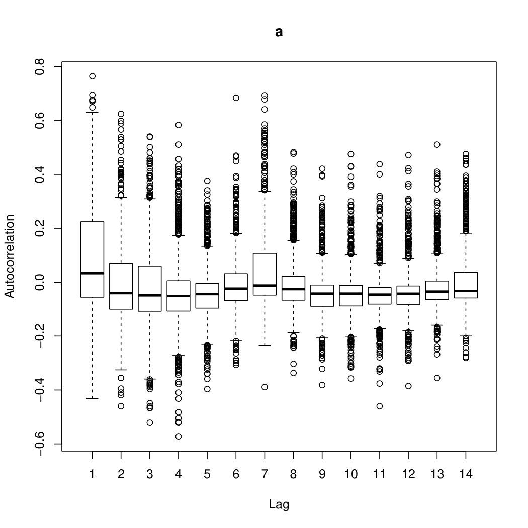 Figure 6
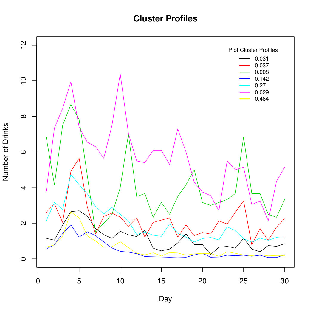 Figure 7
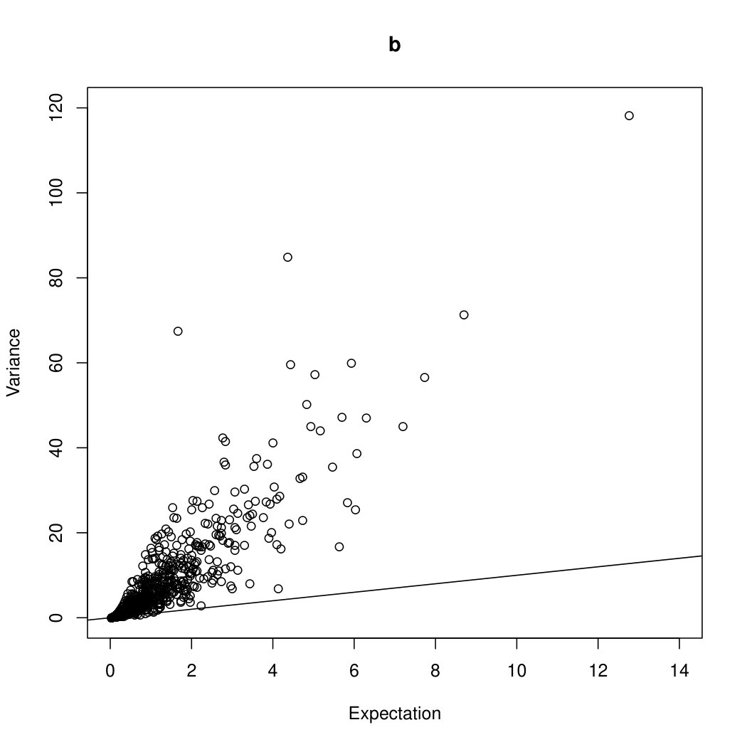 Figure 8
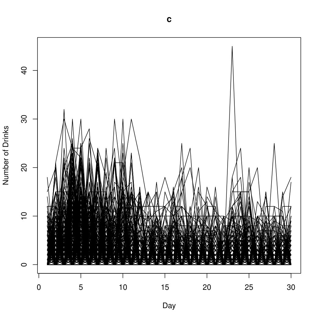 Figure 9
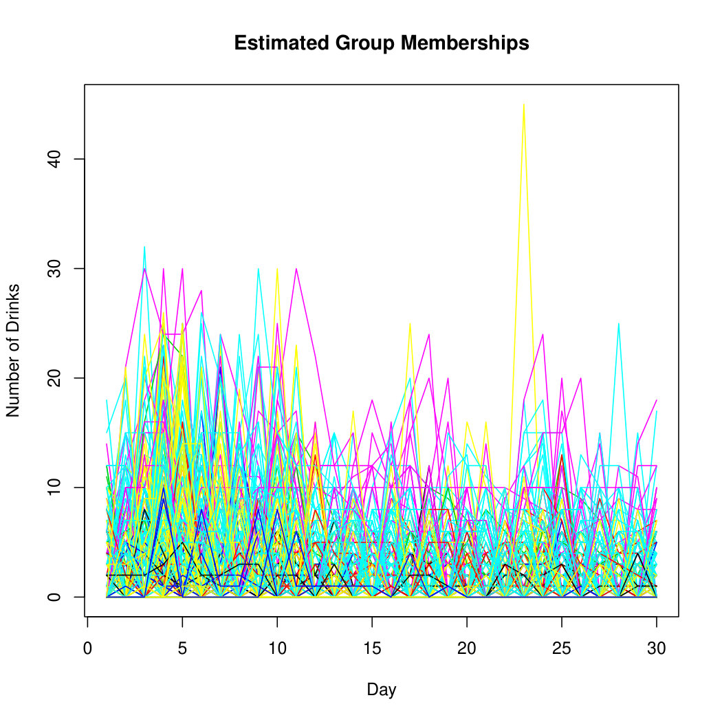 Figure 10
| Clustering Difficulty | True Parameters | Mean Estimated Parameters | Mean ARI (SD) | Classification Table |
|---|---|---|---|---|
| Very Easy | 1 2 1 7500 0 2 0 12500 | |||
| Easy | 1 2 1 7500 0 2 0 12500 | |||
| Moderate | 1 2 3 1 7427 0 73 2 0 12500 0 | |||
| Difficult | 1 2 3 1 7479 8 13 2 1 12499 0 | |||
|
Very
Difficult |
1 2 3 1 6261 1208 31 2 1106 11394 0 |
| Clustering Difficulty | True Parameters | Mean Estimated Parameters | Mean ARI (SD) | Classification Table |
|---|---|---|---|---|
| Very Easy | 1 2 3 1 15000 0 0 2 0 9957 43 | |||
| Easy | 1 2 3 1 15000 0 0 2 0 9963 37 | |||
| Moderate | 1 2 3 1 14988 8 4 2 16 9945 39 | |||
| Difficult | 1 2 3 1 14928 70 2 2 167 9821 12 | |||
|
Very
Difficult |
1 2 1 14884 116 2 267 9733 |
| Clustering Difficulty | FCMdd Classification | Mean Fuzzy ARI (SD) | Mean INAR ARI (SD) |
|---|---|---|---|
| Very Easy | 1 2 3 1 7467 2 31 2 203 11476 821 | ||
| Easy | 1 2 3 1 7194 210 96 2 260 11573 667 | ||
| Moderate | 1 2 3 1 7417 24 59 2 303 10317 1880 | ||
| Difficult | 1 2 3 1 7084 245 171 2 368 11481 651 | ||
| Very Difficult | 1 2 3 1 5181 2100 219 2 3596 8592 312 |
| Clustering Difficulty | FCMdd Classification | Mean Fuzzy ARI (SD) | INAR ARI |
|---|---|---|---|
| Very Easy | 1 2 3 1 14937 5 58 2 132 9695 173 | ||
| Easy | 1 2 3 1 14479 395 126 2 1178 8470 352 | ||
| Moderate | 1 2 3 1 13399 1297 304 2 1626 7975 399 | ||
| Difficult | 1 2 3 1 14104 546 350 2 2067 7378 555 | ||
| Very Difficult | 1 2 3 1 12824 1988 188 2 2305 7395 300 |
Peer Reviews
No public reviews on file for this paper yet. If you reviewed it on a platform where reviews are public (OpenReview, ICLR, NeurIPS, ICML), you can paste yours below so the community can read it here.
Videos
No videos yet. Explain this paper in a talk, walkthrough, or lecture? Add one.
Clustering Discrete-Valued Time Series
Tyler Roick∗, Dimitris Karlis*∗∗* and Paul D. McNicholas∗
(∗Department of Mathematics & Statistics, McMaster University, Ontario, Canada.
*∗∗*Department of Statistics, Athens University of Economics and Business, Athens, Greece.)
Abstract
There is a need for the development of models that are able to account for discreteness in data, along with its time series properties and correlation. Our focus falls on INteger-valued AutoRegressive (INAR) type models. The INAR type models can be used in conjunction with existing model-based clustering techniques to cluster discrete-valued time series data. With the use of a finite mixture model, several existing techniques such as the selection of the number of clusters, estimation using expectation-maximization and model selection are applicable. The proposed model is then demonstrated on real data to illustrate its clustering applications.
Keywords: Finite mixture models; model-based clustering; discrete-valued time series; autoregressive model.
1 Introduction
Consider the case in which we have individuals observed at certain time points. These data are then considered to be comprised of time series, which is a typical panel data situation. Suppose that we are interested in clustering the individuals on a number of, say, clusters based on their observed time series, i.e., based on the data , . Finally, consider that the data are discrete, i.e., , so that we observed discrete-valued time series and we aim at clustering the observations based on the characteristics of their series.
Such data may occur in certain circumstances. For example, consider the situation where individuals count their respective number of drinks per day for a certain time period aiming at identifying different drinking patterns among individuals. The goal is to cluster individuals based on their different drinking patterns. This example will be discussed in depth later. In accident analysis, the goal is to cluster sites with similar accident history in order to develop before and after studies which measure the effect of an intervention. In consumer research, the goal is to use the time series of different consumers and their daily/weekly purchases of a product in order to cluster them based on purchasing patterns. It should be emphasized that since the observation can be a small number of counts, the discreteness of the data needs to be handled with care.
Clustering time series has been a problem that has attracted much research, especially for the case of time series that take continuous values. In this paper, the aim is to establish and apply model-based clustering to appropriately defined discrete valued time series. Model-based clustering for time series has been applied in the past, see the work of Frühwirth-Schnatter and Kaufmann (2008) and the references therein. As opposed to distance-based clustering methods, model-based clustering using finite mixture models extends to time series in a quite natural way. Model-based clustering of time series may be based on many different classes of finite mixture models.
Model-based clustering is a technique for estimating group memberships, in which no observations are a priori labeled, based on parametric finite mixture models. Finite mixture models are based on the assumption that a population is a convex linear combination of a finite number of densities. A random vector is said to arise from a parametric finite mixture distribution if, for all , its density can be written as
[TABLE]
where , such that , is called the th mixing proportion, f_{g}(\mathbf{x}\ |\ \mbox{\boldmath\theta}_{g}) is the th component density, and \mbox{\boldmath\vartheta}=(\pi_{1},\ldots,\pi_{G-1},\mbox{\boldmath\theta}_{1},\ldots,\mbox{\boldmath\theta}_{G}) is the vector of parameters. The component densities f_{1}(\mathbf{x}\ |\ \mbox{\boldmath\theta}_{1}),f_{2}(\mathbf{x}\ |\ \mbox{\boldmath\theta}_{2}),\ldots,f_{G}(\mathbf{x}\ |\ \mbox{\boldmath\theta}_{G}) are usually taken to be of the same type. In our case, due to the discreteness of the data, they will be joint probability mass functions that reflect the underlying time series model. Further details and an in-depth review of model-based clustering can be found in McNicholas (2016a, b).
In this paper, a novel model-based approach for clustering discrete-valued time series is introduced. The approach utilizes a finite mixture of INteger AutoRegressive (hereafter INAR) processes to cluster the data. The work done in the current literature (Pamminger and Frühwirth-Schnatter, 2010; Frühwirth-Schnatter et al., 2011; Frühwirth-Schnatter, 2011) involves model-based clustering of categorical time series based on time-homogeneous first-order Markov chains, model-based clustering of panel or longitudinal data based on finite mixture models, and model-based clustering of categorical time series with multinomial logit classification.
Note that the literature contains certain other approaches for clustering time series. Some such approaches are based on a distance between the series (D’Urso et al., 2019) and others on some other characteristics of the series, e.g., in the periodogram (Caiado et al., 2006) or the autocorrealtion function (D’Urso and Maharaj, 2019). There are also approaches that use a combination of the aforementioned methods such as the approach in Alonso and Peña (2019), where some kind of distance is calculated based on the autocorrelation. Finally, there is work on model-based methods as, for example, in Xiong and Yeung (2004) by using ARMA mixture models and as already mentioned in Frühwirth-Schnatter and Kaufmann (2008). The interested reader can consult very nice reviews by Aghabozorgi et al. (2015) and Caiado et al. (2015), while a more detailed treatment of the problem can be found in Maharaj et al. (2015) and the references therein. We emphasize that our paper focuses on the discrete nature of the data as it is captured by a model-based approach. Existing methods not created for discrete data need to be explained in more detail when the data are counts, as in our case. Later, in Section , we make use of such a method that proposes fuzzy clustering (Izakian et al., 2015) mainly for illustration and comparison purposes.
In Section 2, the framework of our methodology for clustering discrete-valued time series via a mixture of INAR models is presented. The implementation of the EM algorithm for parameter estimation, convergence, initialization, model selection, and performance assessment will be covered. In Section 3, our methodology is applied to both simulated and real data sets, and the results of the application are discussed. In Section 4, a discussion of the work presented throughout this paper is given. Thoughts on the direction of future work are also considered.
2 Methodology
2.1 INAR() model
In recent times, there has been an increasing number of applications for discrete-valued time series models (see Weiss, 2018). The models developed herein are based on a class of INAR models. Certain other models can also be considered for each group.
Definition 2.1**.**
(INAR Process with Binomial Thinning) A discrete time non-negative integer-valued process is said to be a INAR process if it satisfies the recursion
[TABLE]
where , the symbol represents the binomial thinning operator, and is a sequence of non-negative i.i.d. integer-valued random variables with mean and variance . All thinning operations are performed independently of each other and of , and the thinning operations at each time and are independent of .
Definition 2.2**.**
(Binomial Thinning) Let be a non-negative integer-valued random variable and let . Define the random variable
[TABLE]
where the are i.i.d. Bernoulli indicators according to B(1, ), which are also independent of . It can then be said that arises from by binomial thinning.
Binomial thinning was introduced by Steutel and van Harn (1979) to accommodate “self-decomposability” and “stability” for integer-valued time series. This becomes important in regards to the INAR process, which will be discussed following thinning operators. Recall that represents the binomial thinning operator defined in Definition 2.2. Additionally, let and , then some basic properties of binomial thinning, with proofs provided by Freeland (1998) and da Silva (2005), are as follows:
[TABLE]
See Wei\textbeta (2008) for other generalizations of the thinning operator.
The above definition of the INAR model depends on the distribution of the innovation term . The distributional assumptions of result in the marginal properties of the process. For example, assuming a Poisson distribution for we end up with a time series with Poisson marginals, which is perhaps not appropriate to describe data with overdispersion (variance greater than the mean). The model can be extended to what is referred to as the INAR model.
Definition 2.3**.**
(INAR Process) A discrete time non-negative integer-valued process is said to be a INAR process if it satisfies the following recursion
[TABLE]
X_t = ∑_i=1^p α_i ∘X_t-i+ϵ_t,
[TABLE]
where for and .
Further details on extensions of the model can be found in Weiss (2018). Note that the INAR model can be interpreted in two different ways which may cause some confusion. The above specification may either imply applying binomial thinning sequentially and independently or applying a multinomial type of thinning. These two approaches lead to different models in many aspects (e.g., different marginals, different likelihoods).
Finally, we write INAR to denote the model
[TABLE]
In this model, lags up to and including lag are excluded and only lag is considered. The reason for such a model is that we can fit periodic autocorrelations. For example, if the only autocorrelation in daily data comes at order seven, then an INAR model is a parsimonious one. This can also be thought of as a INAR model with .
2.2 The Model
Consider the INAR model defined in Definition 2.1. The conditional likelihood of such a model, being a stationary Markov chain, can be written as
[TABLE]
where is the vector of parameters, refers to the probability of success for binomial thinning, and are the parameters associated with the distribution of the innovation terms. The parameters and refer to the mean and dispersion of the innovations, respectively. Note that, for , the term in (2) refers only to the innovation distribution. Considering the previously given definition of binomial thinning, the conditional distribution of the model can be seen as a convolution between the binomial distribution and that of the distribution of the innovation terms. The conditional likelihoods for INAR() processes are similar to that of (2). The general conditional likelihood where the observations are related at higher-order lag times, assuming the same structure as the INAR process, can be written as
[TABLE]
where the first product of (3) corresponds to the distribution of the innovation terms only. The likelihood in (3) is the likelihood contribution for one individual only. For panel data, the product of all the individual likelihoods must be introduced.
In the model-based clustering scenario, we assume a finite mixture of such likelihoods. Although the observations are assumed to have come from an INAR process, they may come from any finite mixture of INAR processes with equal or different orders. If the INAR processes are of different orders, then the respective clusters are considered to differ with respect to temporal patterns. The observations are said to have come from a mixture of INAR processes included in the model with a specific probability. That is to say that each individual belongs to a specific INAR process which does not change over time, but the process may have different orders. The finite mixture of likelihoods for the INAR model can be written as
[TABLE]
where , such that , are the mixing proportions, refers to the likelihood for the th individual, refers to the likelihood of the th individual coming from the th process, and denotes the parameters of the th INAR process which can be of any order.
The likelihood for each individual is found over time from to . The number of components is considered to be unknown and will be estimated using a criterion (see Section 2.6). The finite mixture of likelihoods in (4) can then be seen to follow a similar structure to the definition of a mixture model given in Section 2.2. An important note here is that the model assumes that each individual has a certain INAR process and differs from the model in Böckenholt (1998), where only the innovation term follows a mixture of distributions. Being a finite mixture model we can estimate it using the expectation-maximization (EM) algorithm as described in the next subsection.
2.3 EM Algorithm
The EM algorithm (Dempster et al., 1977) is an iterative procedure used to find maximum likelihood estimates in the case of missing or incomplete data. Each iteration of the EM algorithm involves two steps, the expectation (E) step and the maximization (M) step. The E-step involves computing the conditional expected value of the complete-data log-likelihood, while the M-step maximizes the expected value of the complete-data log-likelihood with respect to the model parameters. Complete-data refers to the combination of the observed and unobserved data. The E- and M-steps are iterated until convergence is reached — in practice, this means some stopping rule is satisfied (see below).
In straightforward applications of model-based clustering, the complete-data is comprised of the observed data along with the unknown group membership labels , where and
[TABLE]
for and . The estimation of , or specifically of , is the primary objective of model-based clustering.
A well-known approach for determining whether the EM algorithm has converged is by the use of Aitken’s acceleration (Aitken, 1926). The Aitken acceleration procedure estimates the asymptotic maximum log-likelihood at each iteration of the EM algorithm and makes a decision about whether it has converged or not. At iteration , the Aitken acceleration is given by
[TABLE]
where is the log-likelihood value from iteration . An asymptotic (i.e., after many iterations) estimate of the log-likelihood at iteration is given by
[TABLE]
The stopping criterion proposed by Lindsay (1995) suggests that the EM algorithm has converged when
[TABLE]
where is a small value. An alternative stopping criterion was proposed by McNicholas et al. (2010), which suggests that the algorithm has converged when
[TABLE]
for a small value of tolerance . For fixed , the criterion in (6) is at least as strict as (5). Further, the criterion in (6) is at least as strict as the lack of progress criterion, i.e., , in the neighborhood of a maximum (McNicholas et al., 2010).
2.4 Model Fitting
Considering that the model follows a similar structure to that of the definition of a finite mixture model, estimation via the EM algorithm is considered. As the focus of this method is for model-based clustering purposes, the scenario in which there are observations, none of which have known group memberships, is also considered. At each E-step, the component indicator variables are updated using their conditional expected values
[TABLE]
In each M-step, the (conditional) expected value of the complete-data log-likelihood is maximized with respect to the model parameters. The mixing proportions are first updated via
[TABLE]
for , where . Because we do not have a closed form expression, the weighted likelihood
[TABLE]
can be maximized via the optim function in R (R Core Team, 2018) to obtain the model-specific parameters. At each successive iteration of the above steps, the likelihood is increased until a set convergence condition is met. The stopping criterion in (6) is used to determine whether the EM algorithm has converged.
2.5 Initialization
For each number of components , there must be initial values for the . The objective is to obtain the true values of the model parameters to optimize . The ability to obtain good starting values for the parameters proves to be heavily dependent on the distribution of the innovations. In the case of equal dispersion, herein referred to as equidispersion, the innovations are assumed to follow a Poisson distribution.
Equidispersion implies that in
[TABLE]
In the case of overdispersion (), the innovations can be thought to follow a negative binomial distribution. Overdispersion is the result of the variance being larger than the expectation. It is worth noting that the weighted likelihood frequently fails to be optimized if dispersion is not accounted for and Poisson innovations are used. Although very rare, the case of under-dispersion is handled similarly.
In all cases, starting values are obtained with the use of -means clustering. The initial values of the means are taken to be similar to the first group of centers found by -means. The mixing proportions are based on the respective cluster sizes. For , the probability of success, , for the binomial distribution is estimated by minimizing the average of the absolute difference of sums between simulated data and that of the observed data for the clusters found by -means. This is done using the previously estimated values of and , respectively. The simulated data that the observed data is compared to are created using the most influential lag time. A similar approach is used in the case of , although both and must be estimated here. Minimizing the absolute mean of the difference between the observed data and simulated data provides moderately accurate starting values for both. The model proves to be more accurate when initialized in an iterative fashion, meaning that initialization is really only an issue for the smallest number of components fitted. Subsequent numbers of components use the maximized parameter values found when components are fitted with the addition of a new component centered at the mean with a small mixing proportion.
2.6 Model Selection and Performance Assessment
The models for this method are considered to be the possible mixtures of INAR processes. The INAR processes to be included in the mixtures are decided by their respective autocorrelations. For example, in Figure 1, the two most influential autocorrelations are of order one and order seven, respectively. If these were the only two desired autocorrelations to be included in the model, then any mixture of these two autocorrelations may be used. This means that the possible models are mixtures of the form INAR and INAR, where is the number of components and . It is obvious that is restricted by because a negative number of INAR processes cannot be fitted, but as increases so does the total number of possible mixtures.
With the use of mixture models, an objective criterion is needed to select the ‘best’ model. The Bayesian information criterion (BIC; Schwarz, 1978) can be used to select the best model. Given a model with parameters , the Bayesian information criterion can be written
[TABLE]
where is the maximized log-likelihood, is the maximum likelihood estimate of , is the number of free parameters, and is the number of observations. For our model, in the case of Poisson distributed innovations, there are free parameters from the estimation of , from the estimation of , and from the estimation of . Note that, in the case of negative binomial distributed innovations, there are an additional free parameters from the estimation of the dispersion . The number of observations comes from the total amount of time points for all individuals.
Although in a real clustering scenario the true group memberships are not known, the effectiveness of the model will be evaluated through simulated data with known group memberships. The model is evaluated using a cross-tabulation of the maximum a posteriori (MAP) classification of the predicted group memberships versus the true group memberships. Using the results of the cross-tabulation, the performance can be quantified numerically though the use of the adjusted Rand index (ARI; Hubert and Arabie, 1985). The ARI corrects the Rand index (Rand, 1971) for agreement by chance and has an expected value of [math] under random classification and a value of for perfect class agreement.
3 Applications
3.1 Overview
The model developed in Section will now be applied in both simulation studies and real data analyses. An analysis of the results for each application will be carried out. The two simulation studies reflect the different aspects covered throughout Section in regards to equidispersion and overdispersion. For simplicity in the analyses, only the two most influential INAR processes will be considered in the models. The INAR processes to be included in the model will be decided by the most influential autocorrelations at a multitude of different lag times. We will also only consider two possible models in each analysis, i.e., mixtures of INAR and INAR, where and are the most influential autocorrelations, is the number of components, and . Due to two INAR processes and two models being considered, components will not be fitted. This is done for consistency purposes while following the iterative approach mentioned previously and also corresponds to the kind of models used later in the real data analysis.
For each simulated data analysis, simulated data sets will be generated for each of five increasing difficulty scenarios. To increase the challenge in clustering, the parameters of the simulated data will converge together (as the difficulty increases) to bring the clusters closer and create more overlap. Both simulated data analyses will be done in a clustering fashion such that the true group memberships of the data will be taken as unknown. This allows us to assess the performance and classification accuracy using the ARI.
3.2 Simulated Data Analyses
3.2.1 Poisson Innovation Simulated Data
INAR data with Poisson distributed innovations are simulated with increasing difficulty. The true parameters along with the mixing proportions of the two components in each simulation can be found in Table 1. In this case, two-component observations are simulated. The two-component model in this scenario is simulated from a mixture of two INAR. The dimensions of the simulated data are for individuals over times .
Given that the data was simulated from a mixture of two INAR, it is to be expected that autocorrelations at lag and lag would be the most influential autocorrelations. Hence, mixtures of INAR and INAR are used for the model. Because the data have been simulated for Poisson distributed innovations, the dispersion of the data will mainly follow along the Poisson line, where .
For each of five clustering scenarios with different overlapping clusters, components are fit using -means starting values. The tolerance level for convergence is taken to be . The results of each trial can be seen in Table 1 along with corresponding MAP classifications. The BIC in almost all clustering difficulties selects components using a mixture of two INAR and zero INAR as the best model. This is prominent from the collapsed classification tables that can be seen in Table 1. The mean estimated parameters over the simulations in each clustering difficulty are remarkably close to the true parameters with the exception of the dispersion in the very easy, easy, and moderate difficulties. The mean dispersion is very skewed in these three difficulties as it only appears larger than in , , and cases, respectively. The is due to the fact that some Poisson simulated data sets are slightly overdispersed but fitted as if equidispersion were present. The overall difference between true and estimated parameters is very marginal. It can be seen that when a three-component model is selected, it is common that a very small mixing proportion is assigned to that component with parameters that are sensible in light of the first two components. Note, the averages of the third component parameters are reported as an average over the number of cases in which a third component was selected. The mean and standard deviation of the ARI for each of the simulations are reported in Table 1. All scenarios achieve very good results for their respective difficulties. It can be seen from the very difficult clustering scenario that results dwindle slightly. Although, reasonable parameters are found and an overall misclassification rate of is still achieved (Table 1). The classification table presents the true classification as rows and those derived as columns accumulated over the 100 replications (200 observations for each replication, in total 20000 observations classified for the whole experiment).
3.2.2 Negative Binomial Innovation Simulated Data
Following in a similar fashion to Section 3.2.1, INAR data with negative binomial distributed innovations are simulated with increasing difficulty. The true parameters along with the mixing proportions of the two components in each simulation can be found in Table 2. In this case, two-component observations are simulated. The two-component model in this scenario is simulated from a mixture of one INAR and one INAR. The dimensions of the simulated data are for individuals over times .
Given that the data were simulated from the aforementioned mixture, it is to be expected that autocorrelations at lag and lag would be the most influential autocorrelations. Hence, mixtures of INAR and INAR are used for the model. Because the data have been simulated with negative binomial distributed innovations, the dispersion of the data always lies above the Poisson line, thus strongly indicating overdispersion.
For each of five clustering scenarios components are fitted using -means starting values. The tolerance level for convergence is again set to . The results of each trial can be seen in Table 2 along with corresponding MAP classifications. The BIC commonly selects components using a mixture of one INAR and one INAR as the best model. This model is selected in all simulations for the very difficult clustering scenario. For the very easy and easy clustering scenarios, it was seen that good performance could be achieved using a mixture of two INAR and zero INAR. From the collapsed classification tables in Table 2, the BIC has correctly selected the number of components in almost all simulations. Unlike the Poisson distributed innovations, an ARI of over was achieved for all clustering difficulties (Table 2). This is quite remarkable considering that existing clustering methods for time series data are unable to account for overdispersion — see, e.g., Section 3.2.3. The mean estimated parameters for the simulated data with negative binomial distributed innovations appear to be slightly more accurate than the Poisson distributed innovations. There also exists no skewed results as the model is fit for data with overdispersion which is always present in this scenario.
3.2.3 Result Comparison to Fuzzy Clustering
To provide a sensible comparison to the clustering approach developed in Section , we have chosen to compare the simulation study results to that of Fuzzy C-Medoids (FCMdd; Krishnapuram et al., 2001) clustering using dynamic time warping distance (DTW; Berndt and Clifford., 1994). Details of this clustering approach for time series are described in Izakian et al. (2015). In applying this approach, components are fit using random starts and a fuzziness parameter of . The tolerance level for convergence is set to a more strict value than that of the INAR approach, i.e., it is taken to be . This approach is applied to each of the simulated data sets for each of five clustering difficulties in both the equidispersion and overdisperion scenarios. To summarize results, the average ARI values, and the associated standard deviations, are reported alongside collapsed classification tables.
In Table 3, the results of the FCMdd approach for Poisson distributed innovations can be seen. The FCMdd approach performs worse than the INAR approach for all clustering difficulties with a much larger variation in the results. This approach frequently selects the incorrect number of components in numerous simulations for each difficulty. The ability of the FCMdd approach to produce reasonably good results for the first four difficulties can most likely be attributed to the lack of overdispersion present in the data.
In Table 4, the results of the FCMdd approach for negative binomial distributed innovations are presented. It can be seen that the INAR approach outperforms FCMdd for all five clustering difficulties to a greater extent than for the Poisson distributed innovations. The FCMdd approach is unable to account for overdispersion in the data. Other time series properties, and the possibility of large amounts of zeros in the data, may also be unaccounted for. Overall, considering that factors such as overdispersion are commonly seen in real data, the INAR model can be considered far superior when it comes to clustering discrete-valued time series.
3.3 Real Data Analyses
3.3.1 Alcohol Timeline Followback Data
The timeline followback (TLFB) method (Sobell et al., 1986) is a tool used to assess subjects’ daily alcohol consumption. The alcohol TLFB data we consider (Atkins et al., 2013) is available at www.researchgate.net, and comes from a larger study aimed at event-specific prevention. The event-specific prevention here refers to intensive daily drinking habits around a number of people’s twenty-first birthdays. This data also includes extreme drinking events relative to a random sample of students’ drinking (Neighbors et al., 2010). Estimates of daily drinking were evaluated for clinical and nonclinical populations; e.g., adolescents, adults, college students, alcoholics of different severity, and normal male and female drinkers in the general population. Using a calendar, subjects provided retrospective estimates of their daily drinking over a specified time period. The original focus of the assessment was to study the gender, whether the subject is in a fraternity/sorority or neither (“greek status”), and period of the week in which the drinking occurred. Our focus will be solely on the number of drinks and what can be inferred about the clusters found.
The data are composed of individuals who listed their respective number of drinks over a -day period. There were individuals who did not finish the study, and we will only consider the individuals for which the data were fully recorded. Taking a closer look at the data, Figure 1 shows box plots of the autocorrelations. From these box plots, only mixtures of INAR and INAR will be considered in the model. It can be seen from Figure 1 that overdispersion is present in the TLFB data.
For the alcohol TLFB data, components are fitted using -means starting values. The tolerance level for convergence is taken to be . The BIC selects components using a mixture of seven INAR and zero INAR processes. This suggests that weekly drinking habits are not very prominent in the data. Figure 1 shows the raw, i.e., unlabelled, data. Figure 1 shows the estimated group memberships of the TLFB data, and Figure 1 shows the respective cluster profiles of the estimated group memberships. From the seven cluster profiles present in Figure 1, there seem to be individuals on very extreme ends of the spectrum. The blue profile appears to be individuals who drank around the times of their twenty-first birthday and returned to not drinking throughout the remainder of the study. The yellow profile, although very similar to the blue profile, appears to be individuals who continued drinking lightly after the specified event. The black, red, and turquoise profiles appear to be individuals with heavier drinking habits, but at a variety of different quantities. The green and purple profiles appear to be individuals with very heavy drinking habits that occur on a regular basis. The differences in cluster profiles could perhaps have to do with the individuals’ alcohol tolerance level, or with attendance at other social gatherings besides the time around their twenty-first birthday.
3.3.2 Long Distance Running Strategy Data
This long distance running strategy (LDRS) data comes from the International Association of Ultrarunners (IAU) World Championship held in Katowice, Poland. The dataset is available at maths.ucd.ie/brendan/data/24H.xlsx. Ultrarunners are individuals who compete in ultra-marathons, which are considered to be any race that is longer than miles or km. The types of races include km, km, hour, hour, hour, and hour races. The LDRS data considered herein is composed of individuals who participated in a (consecutive) hour race. In such a race, the number of cumulative laps is recorded at the end of each hour, and the individual with the greatest amount of laps at the end of the hour period is declared the winner. There were runners who were unable to complete a single lap and/or participate in the race. These runners have been excluded from the data so that only the runners who completed at least one lap will be considered in this analysis. Although variables for age, country of origin, and gender are provided, we do not consider them in our model because our goal while clustering these data is to analyze the different running strategies used by ultrarunners. The three main strategies to running ultra-marathons can be summarized as: running with a consistent pace for the entire race; starting with a fast pace and slowing down earlier; and starting at a consistent pace, slowing down through the middle of the race, and finishing with a fast pace.
Taking a closer look at the data, Figure 2 shows box plots of the autocorrelations. From these box plots, only mixtures of INAR and INAR will be considered in the model. It can be seen from Figure 2 that overdispersion is clearly present in the LDRS data. This suggests that negative binomial distributed innovations should be considered.
For the LDRS data, components are fitted using -means starting values. The tolerance level for convergence is again taken to be . The BIC selects components using a mixture of five INAR and zero INAR. This implies that runner strategies are discovered on a lap-to-lap basis. Figure 2 shows the raw, i.e., unlabelled, data. Figure 2 shows the estimated group memberships of the LDRS data and Figure 2 shows the respective cluster profiles of the estimated group memberships. From the five cluster profiles present in Figure 2, we see that the turquoise and black profiles are the consistent pace runners previously mentioned. The green profile represents the runners who start with a fast pace and slow down earlier. The red profile is runners who start fast relative to their capabilities and slow down throughout the middle. It looks as if these runners attempted to pick up their pace at the end but were unsuccessful. The blue profile looks to be runners who dropped out early due to their running capabilities as no real strategy is present.
4 Discussion
A model-based approach for clustering discrete-valued time series has been introduced. The model parameters were estimated using the EM algorithm. A stopping criterion based on Aitken acceleration was used to determine if the model had converged. The model-based technique was applied to both simulated and real data to illustrate its clustering capabilities. Model selection was done using the BIC and, for simulated data, performance assessment was carried out using the ARI. In the applications to simulated data, the technique performed very well for a variety of scenarios with different overlapping among the clusters. Both equidispersion and overdispersion cases were present in the simulated data. In the application to real data, two true clustering scenarios — i.e., where there are no “true” groups or labels — were considered. The technique performed appropriately and reasonable numbers of clusters were found for the obscure relationships within the data.
This novel model-based approach for clustering discrete-valued time series presents many different directions that could be taken in future work. Some of the more relevant directions to be taken include extending the INAR model to include multivariate time series of counts and using the generalized INAR model (see Definition 2.3) where all lags would be considered in the model. Other directions include expanding the model-based approach to include other integer-valued models, e.g., a mixture of INARCH models, and the improvement of computational aspects, e.g., the maximization step in the EM algorithm is time consuming.
While the existing literature contains other approaches for clustering time series, we have focused on the discrete nature of the data. The existing literature ignores this property and, hence, it is of interest to examine the behaviour of distance-based and other related methods on discrete-valued data. Applying one such method herein, we found that our approach has some advantages but a more wide ranging comparison would be useful. For example, one may attempt to use the frequency domain and apply spectral analysis to the integer valued time series for clustering purposes.
Acknowledgements
The authors are grateful to anonymous reviewers for their very helpful comments. This work was supported by the Canada Research Chairs program and an E.W.R. Steacie Memorial Fellowship (McNicholas).
The reference list from the paper itself. Each links out to its DOI / PubMed record.
- 1Aghabozorgi et al. (2015) Aghabozorgi, S., A. S. Shirkhorshidi, and T. Y. Wah (2015). Time-series clustering–A decade review. Information Systems 53 , 16–38.
- 2Aitken (1926) Aitken, A. C. (1926). A series formula for the roots of algebraic and transcendental equations. Proceedings of the Royal Society of Edinburgh 45 , 14–22.
- 3Alonso and Peña (2019) Alonso, A., and D. Peña (2019). Clustering time series by linear dependency. Statistics and Computing 29 (4), 655–676.
- 4Atkins et al. (2013) Atkins, D. C., S. A. Baldwin, C. Zheng, R. J. Gallop, and C. Neighbors (2013). A tutorial on count regression and zero–altered count models for longitudinal substance use data. Psychology of Addictive Behaviors: Journal of the Society of Psychologists in Addictive Behaviors 27 (1), 166–177.
- 5Berndt and Clifford. (1994) Berndt, D., and J. Clifford (1994). Using dynamic time warping to find patterns in time series. In Proceedings of the AAAI-94 Workshop Knowledge Discovery in Databases , 359–370.
- 6Böckenholt (1998) Böckenholt, U. (1998). Mixed INAR (1) Poisson regression models: Analyzing heterogeneity and serial dependencies in longitudinal count data. Journal of Econometrics 89 (1-2), 317–338.
- 7Böhning et al. (1994) Böhning, D., E. Dietz, R. Schaub, P. Schlattmann, and B. Lindsay (1994). The distribution of the likelihood ratio for mixtures of densities from the one-parameter exponential family. Annals of the Institute of Statistical Mathematics 46 , 373–388.
- 8Caiado et al. (2006) Caiado, J., N. Crato, and D. Peña (2006). A periodogram-based metric for time series classification. Computational Statistics & Data Analysis 50 (10), 2668–2684.