On Roth type conditions, duality and central Birkhoff sums for i.e.m
Stefano Marmi, Corinna Ulcigrai, Jean-Christophe Yoccoz

TL;DR
This paper introduces new Diophantine conditions on interval exchange maps and translation surfaces, extending previous results on cohomological equations and analyzing distributional limit shapes for functions with subpolynomial deviations.
Contribution
It defines the absolute and dual Roth type conditions, extending cohomological results and constructing distributional limit shapes for specific classes of functions.
Findings
Extended cohomological equation results to absolute Roth type i.e.m.
Constructed distributional limit shapes under dual Roth type condition.
Linked limit shapes to subpolynomial deviations of ergodic averages.
Abstract
We introduce two Diophantine conditions on rotation numbers of interval exchange maps (i.e.m) and translation surfaces: the \emph{absolute Roth type condition} is a weakening of the notion of Roth type i.e.m., while the \emph{dual Roth type} condition is a condition on the \emph{backward} rotation number of a translation surface. We show that results on the cohomological equation previously proved in \cite{MY} for restricted Roth type i.e.m. (on the solvability under finitely many obstructions and the regularity of the solutions) can be extended to restricted \emph{absolute} Roth type i.e.m. Under the dual Roth type condition, we associate to a class of functions with \emph{subpolynomial} deviations of ergodic averages (corresponding to relative homology classes) \emph{distributional} limit shapes, which are constructed in a similar way to the \emph{limit shapes} of Birkhoff sums…
Click any figure to enlarge with its caption.
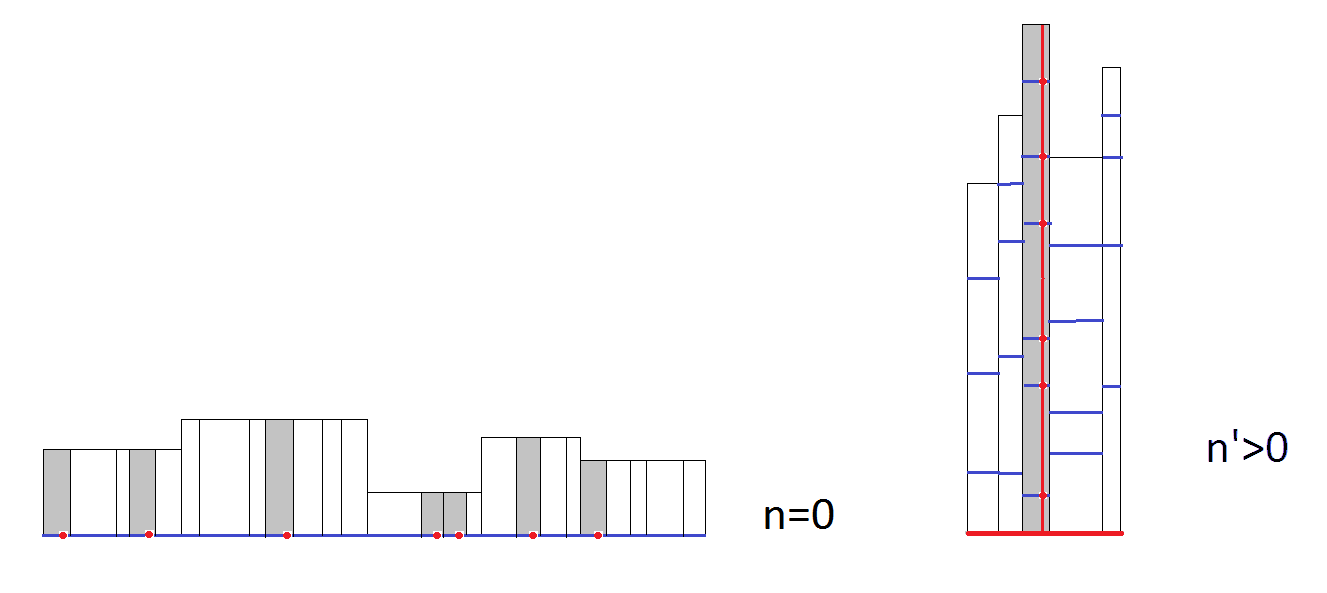 Figure 1
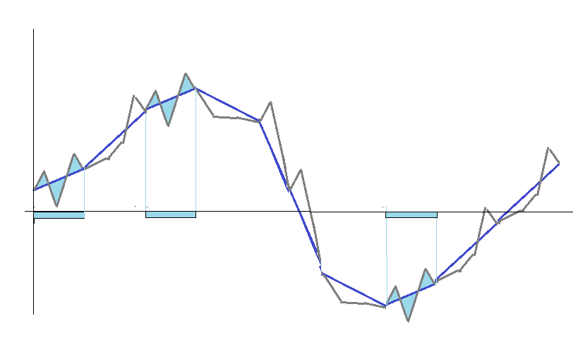 Figure 2
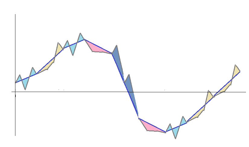 Figure 3
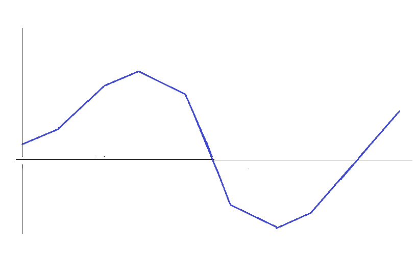 Figure 4
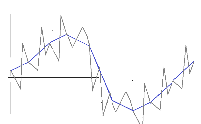 Figure 5
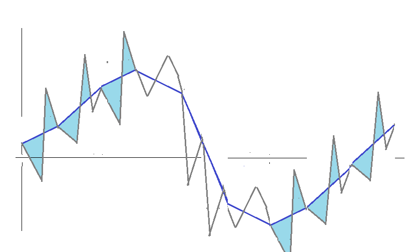 Figure 6
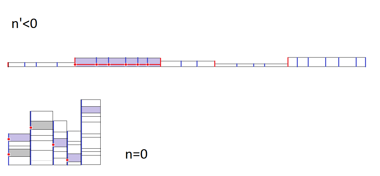 Figure 7
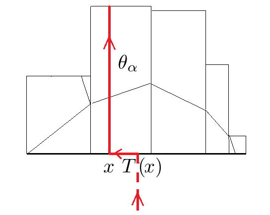 Figure 8
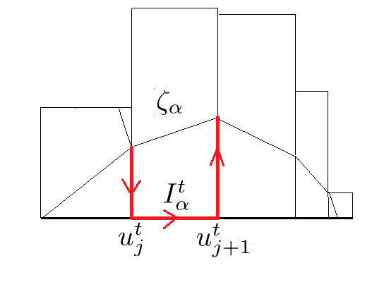 Figure 9
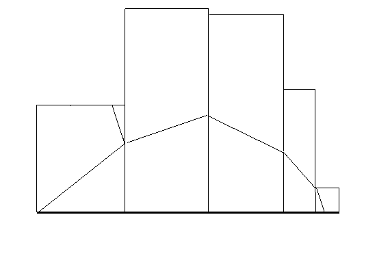 Figure 10
Peer Reviews
No public reviews on file for this paper yet. If you reviewed it on a platform where reviews are public (OpenReview, ICLR, NeurIPS, ICML), you can paste yours below so the community can read it here.
Videos
No videos yet. Explain this paper in a talk, walkthrough, or lecture? Add one.
Taxonomy
TopicsMathematical Dynamics and Fractals · Topological and Geometric Data Analysis · Geometric and Algebraic Topology
111Here we summarize the timeline connecting the various texts written by J.C.Y. reporting on our joint work and on which the writing of this article is based. The collaboration between the three authors began during a stay of the three of us at the Mittag-Leffler Institute in April and June 2010 and again at K.T.H. in Stockholm in February 2011. It then continued with frequent meetings until the last year of life of Jean-Christophe (the last mathematical discussions of the coauthors on this research project date of July 2015, when C.U. met J.C.Y. at CIRM, and September 2015 when S.M. visited J.C.Y. in Paris). In August 2010 J.C.Y. wrote a first text (12 pages) containing the results obtained on dual Birkhoff sums with the title ”On Birkhoff sums for i.e.m.” (a further version of the same text was written in March 2011). This constitutes the heart of Section 4 of this paper. Notable progress was made during a visit of S.M. and J.C.Y. to C.U. in Bristol in October 2014, when the homological interpretation emerged and J.C.Y. wrote a new version of this draft introducing the notion of KZ-hyperbolic translation surfaces (this homological interpretation is included in Section 6). Motivated by the discussions in Bristol, the notion of absolute Roth type i.e.m. emerged and was developed during further meetings in of S.M. with J.C.Y. in Paris in December 2014, March 2015 and September 2015. This notion, together with the completeness of backward rotation numbers, is the object of the text ”Absolute Roth Type and Backward Rotation Number” (14 pages) written by J.C.Y. in April 2015. This text formed the basis for Section 3 and parts of it are here included as two Appendixes (Appendix A and Appendix B). The final version of this manuscript was prepared by S.M. and C.U. who are fully and solely responsible for any mistake or imprecision. Jean-Christophe discussed publicly the results obtained in our collaboration in his talk “Problèmes de petits diviseurs pour les échanges d’intervalles” on May 20, 2015 given at the “Journée Surfaces plates” held at the Institut Galilée of the University of Paris 13 (as Carlos Matheus informed us) and also during his talk “Diophantine conditions for interval exchange map” on September 28, 2015 given in Oxford as part of the Worshop Geometry and Dynamics on Moduli Spaces at the 2015 Clay Research conference.
On Roth type conditions, duality and central Birkhoff sums for i.e.m
Stefano Marmi
Scuola Normale Superiore
Piazza dei Cavalieri, 7
56126
Pisa
Italy
,
Corinna Ulcigrai
Institut für Mathematik
Universität Zürich
Winterthurerstrasse 190
CH-8057
Zürich
Switzerland
and School of Mathematics
University of Bristol
University Walk
Bristol
BS8 1TW
United Kingdom
and
Jean-Christophe Yoccoz
(Date: October 27, 2017)
Abstract.
We introduce two Diophantine conditions on rotation numbers of interval exchange maps (i.e.m) and translation surfaces: the absolute Roth type condition is a weakening of the notion of Roth type i.e.m., while the dual Roth type condition is a condition on the backward rotation number of a translation surface. We show that results on the cohomological equation previously proved in [MY] for restricted Roth type i.e.m. (on the solvability under finitely many obstructions and the regularity of the solutions) can be extended to restricted absolute Roth type i.e.m. Under the dual Roth type condition, we associate to a class of functions with subpolynomial deviations of ergodic averages (corresponding to relative homology classes) distributional limit shapes, which are constructed in a similar way to the limit shapes of Birkhoff sums associated in [MMY2] to functions which correspond to positive Lyapunov exponents.
Contents
-
2.3 A step of Rauzy–Veech algorithm, Rauzy Veech diagrams and Rauzy-Veech matrices
-
2.4 Iterations of the Rauzy-Veech map and the Zorich algorithm
-
2.6 Special Birkhoff sums and the extended Kontsevich-Zorich cocycle
-
3.5 Results on the cohomological equation for absolute Roth type i.e.m.
-
3.6 Results on the cohomological equation for translation surfeces in a.e. direction
-
4.1 Backward Rauzy-Veech induction and backward rotation numbers
-
4.5 Estimates on dual special Birkhoff sums of Hölder functions
-
6.1 Bases of homology associated to the Rauzy-Veech algorithm
-
B Adaptation of the proofs of results on cohomological equation for absolute Roth type i.e.m.
-
B.4 Adaptation of the proof of Theorems 3.10 and 3.11 in [MY]
1. Introduction
Diophantine conditions play a central role in the study of the dynamics of rotations of the circle, diffeomorphisms of the circle and more in general area-preserving flows on tori. These conditions, which convey information on how well a rotation number can be approximated by rationals (and hence on small divisors problems), are often expressed in terms of growth rates for the entries of the continued fraction expansion of .
In the study of dynamics on surfaces, one often requires similar Diophantine conditions on interval exchange maps and linear flows. Passing from genus one to higher genus, a natural generalization of linear flows on tori is indeed provided by linear flows on translation surfaces (see 2.2 for definitions); interval exchange maps, which will be shortened throughout this paper by i.e.m., are piecewise isometries which, analogously to rotations in genus one, arise are Poincaré maps of linear flows (see 2.1 for the definition). An algorithm which plays in this context an analogous role to the continued fraction expansion is the Rauzy-Veech induction, first introduced [Rau, Ve1] and used since then as an essential tool for proving many results on the ergodic and spectral properties of i.e.m., flows on surfaces and rational billiards, see for example [Ve2, Zo3, MMY1, Fo3, AvFo, AtFo, Ul1, Ul2, MMY3, Ch, Bu2, Rav, KKU].
Diophantine conditions on i.e.m. can be prescribed imposing conditions on the behaviour of the Rauzy-Veech induction matrices and the related (extended) Kontsevich-Zorich cocycle. In this spirit, in their work [MMY1] on the cohomological equation for i.e.m., S. M. , P. Moussa and J.-C. Y., define a Diophantine condition on i.e.m. which generalize the notion of Roth type rotation and under which they show that the cohomological equation can be solved under finitely many obstructions (see Theorem 3.14 for a generalized statement). After Forni’s celebrated paper [Fo1] on the cohomological equation associated to linear flows on surfaces of higher genus, this was the first result giving an explicit diophantine condition sufficient to guarantee the existence of a solution to the cohomological equation. The i.e.m. which satify this condition are called Roth type i.e.m. (or i.e.m. of Roth type) and have full measure (as shown in [MMY1], see also [MMM] for the sketch of a simpler proof based on the results in [AGY]). A reformulation and a strenghthening of the Roth type condition (namely, restricted Roth type) were then defined in [MMY3] also for generalized i.e.m. and provide the Diophantine condition under which a linearization result is proved in [MMY3].
Two new Diophantine conditions related to the Roth type condition for i.e.m. are introduced in this paper, for the applications that we explain in § 1.1 and § 1.2 below. More precisely (in 3) we introduce the notion of absolute Roth type i.e.m., thus defining a class of i.e.m. which include and generalize Roth type i.e.m. but for which the results mentioned before on linearization and the cohomological equation still hold. We then define the notion of dual Roth type for a translation surface (or more precisely, for its suspension data or backward rotation number, see 4). This is a Diophantine condition which is dual to the Roth type condition for i.e.m. in a sense which will be made precise further on (see 4 and 6). Let us now explain the motivation for introducing these conditions and the results which we proved assuming them, starting with the notion of dual Roth type.
1.1. Dual Roth type and distributional limit shapes.
Results on deviations of ergodic averages and ergodic integrals are a central part of the study of i.e.m. and translation flows, see for example the works by Zorich [Zo3, Zo2], Forni [Fo2], Avila-Viana [AV] and Bufetov [Bu2] among others. Deviations of ergodic averages, i.e. the oscillations of the Birkhoff sum of a function of zero average over the orbit of (typical) point under a i.e.m. are of polynomial nature. In [Zo3] Zorich shows for example that for a typical i.e.m. and any mean-zero function constant on the intervals exchanged by , we have for some power exponent ; more precisely for a full measure set of there exists such that for all ,
[TABLE]
Remark also that if is a coboundary for with bounded transfer function, i.e. where the transfer function is bounded, then Birkhoff sums are uniformely bounded (and in particular ). The power exponent can be understood in terms of Lyapunov exponents of (a suitable acceleration) of the Kontsevich-Zorich cocycle associated to the Rauzy-Veech induction [Zo1, Zo2]. In particular, is a ratio of Lyapunov exponents and depends on the position of the piecewise constant function (identified with a vector of ) with respect to the Oseledets filtration of the Kontsevich-Zorich cocycle. Using this interpretation, it follows from the work of Forni [Fo2] (see also [AV]) that, for a typical choice of function , is positive; furthermore one also has as an immediate consequence of the work of Veech [Ve5] (see also [Fo2] for a more general result)). A powerful result of similar nature for ergodic integrals of smooth area-preserving flows was proved by Forni in [Fo2]: the power spectrum of ergodic integrals is related to Lyapunov exponents of the Kontsevich-Zorich cocycle and Forni’s invariant distributions.
A finer analysis of the behaviour of Birkhoff sums or integrals, beyond the size of oscillations, appears in the works [Bu2, MMY2]. In [MMY2], motivated by the study of wandering intervals in affine i.e.m., S. M., P. Moussa and J.C.Y. introduced an object called limit shape and used it to describe the shape of ergodic sums (see 3.4 and 3.7.3 in [MMY2]). Roughly speaking these are obtained by looking at suitably rescaled Birkhoff sums, where time is renormalized according to the leading Laypunov exponent of the Kontsevich-Zorich cocycle, whereas the range of the sum is renormalized using one of the other positive exponents, according to the choice of . After this double rescaling one obtains a sequence of shapes exponentially converging (in the Hausdorff metric) to the graph of a Hölder function. In [Bu2], Bufetov studies limit theorems for ergodic integrals of translation flows and describe weak limit distributions in terms of objects that he calls Hölder cocycles (or, in the context of Markov compacta, finitely-additive measures) and turn out to be dual to Forni’s invariant distributions (see [Bu2] for details). We remark that limit shapes and Hölder cocycles, despite having been introduced independently, are intrinsically related: limit shapes are essentially graphs of Hölder cocycles along flow leaves. Let us remark that similar results can also be proved for horocycle flows on negatively curved surfaces, see [BuFo] were the existence of Hölder cocycles is proved in this context.
Both limit shapes and Hölder cocycles are associated to functions which display truly polynomial deviations, i.e. for which the exponent in (1.1) is strictly positive. More precisely, from the work of Forni [Fo2] and Avila-Viana [AV] it follows that for a typical i.e.m. with exchanged subintervals, the extended Kontsevich-Zorich cocycle has positive Lyapunov exponents, negative and zero ones, where and and can be computed from the combinatorics of ( is the genus and is the number of marked points of any translation surface which suspends , see § 2.2). For typical i.e.m. , functions which are coboundaries with bounded transfer functions and hence have bounded Birkhoff sums, can be associated to the stable space of the Kontsevich-Zorich cocycle, which correspond to negative Lyapunov exponents.
We construct in this paper objects similar to the limit shapes introduced in [MMY2] for functions which display subpolynomial deviations of ergodic averages, i.e. functions for which in (1.1) is equal to zero, but are not coboundaries. An important example of this type of function arise when considering rotations of the circle (which correspond to i.e.m. with ) and a mean zero function , where is the characteristic function of the interval . The function can be seen as a piecewise constant function on a i.e.m. with . It is well known that in this case display logarithmic deviations (which can be described for example in terms of the Ostrowski expansion of with respect to , see for example [BI]). Results on the subdiffusive behaviour of these Birkhoff sums were proved for example in [H, CIL, CL] (see also [BBH] for a related result in the context of substitutions). Celebrated results on limit distributions for the Birkhoff sums under additional randomness were proved for example by Kesten in [Ke1, Ke2] (where the rotation number is randomized) and by Beck in [Be1, Be2] (where time is randomized, see also [DS1, PS, BrUl, DS3] for recent extensions of Beck’s temporal limit distribution results and [DS1, DS2] for results in the context of horocycle flows).
More in general, we show that for a typical i.e.m. (for any number of exchanged intervals ) the characteristic function can be corrected by adding a function constant on the intervals exchanged by in order to display subpolynomial deviations (see Propostion 5.3) and hence these seem to be natural functions for future investigations towards a generalizations of Kesten’s and Beck’s results. Functions with subpolynomial deviations can more generally be associated to relative homology classes in where is a (typical) translation surface with conical singularities (see 6).
We prove in § 4 that for a full measure set of translation surfaces, to each function with subpolynomial deviations (or more in general, in § 6, to each relative homology class with subpolynomial deviations), we can associate limit distribution on Hölder functions, which is constructed in a similar way to the limit shapes in [MMY2] (see 5.2 and 5.4 for details). More precisely, limit shapes in [MMY2] are Hölder functions defined as pointwise limit of a sequence of piecewise affine functions obtained by plotting suitably rescaled graphs of Birkhoff sums. Convergence exploits positivity of the Lyapunov exponent, which implies that oscillations on different scales are of exponentially smaller orders. We define similarly a sequence of piecewise affine functions in our setup, but they fail to converge pointwise since all oscillations are of the same magnitude. We prove on the other hand that there is convergence in the sense of distributions, when integrating these graphs against Hölder continuous functions (see Theorem 5.6).
The Diophantine condition that we need to ensure distributional convergence of this sequence of piecewise affine functions turns out to be a Roth type-like condition, but not for the usual Kontsevich-Zorich cocycle, but for a dual cocycle. This is the (weak) dual Roth type condition that we define in § 4.3. In the proof of convergence, we also need to introduce the notion of dual special Birkhoff sums (see § 4.2). This is based on a duality between horizontal and vertical flow and future and past of the Teichmueller geodesic flow. The same duality is also exploited crucially in the paper by Bufetov [Bu2]. This duality has also a homological intepretation, which we explain in Section 6.
The construction of limit distributions can also be done at the level of homology bases, as explain in Section 6. Distributional limit objects can hence be associated to relative homology classes which have non trivial image by the boundary operator (see . In view of the connection between the limit shapes in [MMY2] and Bufetov’s Hölder cocycles [Bu2] and the duality of the latter and Forni’s invariant distributions (explained in [Bu2], see ADD), our distributional limit objects are presumably connected to invariant distributions in relative homology.
1.2. Absolute Roth type
To motivate the notion of absolute Roth type i.e.m., consider the following example. Let be an interval contained in the domain of an i.e.m. and let be the (possibly corrected, as explained above) characteristic function of . To study the Birkhoff sums of under , it is convenient to add the discontinuity of as marked point (or fake discontinuity), so that the function can be considered as function which is constant over the subintervals exchanged by an i.e.m. of of intervals. It is natural for many questions to fix and vary the i.e.m. . One would hence like to exploit a Diophantine condition on which only depends on the underlying and not on the position of the fake discontinuity .
Let us recall that the number of exchanged intervals coincides with the dimension of the relative homology , where is any translation surface which suspends the i.e.m. (see § 2.2 for definitions) and is the set of conical singularities of . The Roth type condition for i.e.m. is defined in terms of the Rauzy-Veech cocycle, which acts on the relative homology . If in the above example is such that , where is the genus of , i.e. equals the dimension of the absolute homology , the growth of , where is a corrected characteristic function, is given by the growth of a relative homology class in , where suspends and has singularities . One would hence like to introduce Diophantine conditions on which depends only on the absolute homology of .
These considerations led us to define the notion of absolute Roth type i.e.m. (given in § 3). This is a Diophantine condition on an i.e.m. defined in terms of the Rauzy-Veech cocycle, and hence on the action on , but which depends on how the cocycle acts on the absolute homology , which can be identified with a subspace of defined in terms of the combinatorial data of (see § 3 for details). We stress that the absolute Roth type condition is weaker than Roth type, i.e. Roth type i.e.m. satisfy the absolute Roth type condition (see Lemma 3.6 in § 3.3).
While we were thinking of this notion, Chaika and Eskin [CE] proved a result on Oseledets genericity of the Kontsevich-Zorich cocycle which, as an application, implies that given any translation surface , for a.e. direction the i.e.m. obtained as Poincaré maps of the linear flow in direction to a segment in good position (see § 2.2 for definitions) satisfy the absolute Roth type condition. This motivated us to prove that several of the results on the cohomological equation for i.e.m. of (restricted) Roth type, in particular the main results in [MY], are still valid under the weaker (restricted) absolute Roth type condition. These results are presented in § 3.5 (see also § 3.6 and Appendix B).
1.3. Outline of the paper
We first recall background material, in particular definitions and notations for i.e.m and Rauzy Veech induction (see Section 2). The reader who is already familiar with this can skip to Section 2.8 where we simply summarize the notation.
In Section 3 we first recall the Roth type condition introduced by [MMY1] and we then define absolute Roth type. We then states the results, first proved for Roth type, that still hold under this weaker condition. We prove in this section two crucial estimates that shows that Roth type allows to control the lengths of inducing subintervals for the positive acceleration of Rauzy-Veech induction. The proofs of the results which extend from Roth type to absolute Roth type can then be adapted with minor modifications, which, for completeness, we discuss in an appendix (see Appendix B). We then recall the result by Chaika and Eskin in [CE] and get as a Corollary that the results on the cohomological equation holds for every surface in a.e. direction.
In Section 4 we introduce the second variation of Roth type condition studied in this paper, namely dual Roth type. We first introduce the notion of dual Birkhoff sums, which are used to give the definition. We also prove that some classical results, in particular estimates on the growth of special Birkhoff sums of BV fucntions, also holds for special dual Birkhoff sums under this dual Roth type condition.
In Section 5 we study a distributional analogue of limit shapes for functions with subpolynomial deviations of ergodic averages. We first show how a natural class of functions belonging to the central space of the can be obtained by correcting indicatrix functions. We then define the affine graphs which plot the behaviour of central Birkhoff sums. Under the Roth type DC that we introduced in the previous section, we when show that these graphs converge in the sense of distributions (see Theorem 5.6).
Finally, in Section 6, we give a homological interpretation of distributional limit shapes. We define suitable dual bases of relative homology and show that the graphs which we studied in the previous section and their convergence have a homological interpretation.
The Appendix A contain the involved proof that backward rotation numbers are infinitely complete. The Appendix B, as already mentioned, contains a summary of the structure of the proof of the results on the cohomological equation with an indication of the changes one has to do to adapet them to absolute Roth type i.e.m.
1.4. Acknowledgements
We would like to thank Jon Chaika, Alex Eskin and Carlos Matheus for several useful discussions. We also thank the anonimous referee for useful comments. C.U. is partially supported by the ERC Starting Grant ChaParDyn and also acknowledges the support of the Leverhulme Trust through a Leverhulme Prize and the Royal Society and the Wolfson Foundation through a Royal Society Wolfson Research Merit Award. S.M. acknowledges support from UnicreditBank through the Dynamics and Information Research Institute at the Scuola Normale Superiore. The authors would like thank the University of Bristol, Centro di Ricerca Matematica Ennio de Giorgi, Mittag-Leffler Institute and IHES for hospitality during the visits that made this collaboration possible. The research leading to these results has received funding from the European Research Council under the European Union Seventh Framework Program (FP/2007-2013) / ERC Grant Agreement n. 335989.
2. Backgound material and notations
In this section we recall basic definitions and notation for interval exchange maps and Rauzy-Veech induction. We refer to the lecture notes [Yo1, Yo2, Yo4, Zo1] for further information. The reader who is already familiar with this material might want to skip it and to refer to § 2.8 which provides a brief summary of the notation used.
2.1. Interval exchange maps
Let be a bounded open interval. An interval exchange map (i.e.m) i.e.m. on is defined by the following data. Let be an alphabet with symbols. Consider two partitions (modulo [math]) of into open intervals indexed by (the top and bottom partitions):
[TABLE]
such that for every . The map is defined on so that its restriction to each is a translation onto the corresponding . The partitions are determined by combinatorial data on one side, lengths on the other side, as follows. The combinatorial data is a pair of bijections from onto which indicates in which order the intervals are met in the top and in the bottom partition respectively. We always assume that the combinatorial data are irreducible: for , we have
[TABLE]
The length data prescribe the lengths of the partition elements, i.e. for . The i.e.m. determined by these data acts on ; the subintervals of the top partition are
[TABLE]
and those in the bottom partition are
[TABLE]
We also write simply for , and refer to them as the *intervals exchanged by * (or simply exchanged intervals). The i.e.m sends on by the translation , where the translation vector is given by
[TABLE]
and is the antisymmetric matrix associated by the combinatorial data defined by
[TABLE]
The points separating the are called the *singularities * of . The points separating the are called the singularities of . We also define so that . We will also write and when we want to stress the dependence on . The action of on can be extended to by right-continuity. A connection is a triple , where is a nonnegative integer, such that .
2.2. Translation surfaces and suspension data
Let be a compact connected orientable topological surface of genus and let be a non-empty finite subset of . A structure of translation surface on is a maximal atlas for of charts by open sets of which satisfies two properties: any coordinate change between two charts is locally a translation of and for every , there exists an integer and a ramified covering of degree such that every injective restriction of is a chart of . Here and are neighborhoods respectively of and [math].
A translation surface structure naturally provides a complex structure and an holomorphic -form which does not vanish on and has at each point a zero of order . It also provides a flat metric on : the metric exhibits a (true) singularity at each such that and the total angle around each is . The genus of the surface and the order of the zeros of are related by the Riemann-Roch formula .
The geodesic flow of the flat metric on gives rise to a -parameter family of constant unitary directional flows on , called linear flows, containing in particular a vertical flow and a horizontal flow . An orbit of the vertical (horizontal) flow which ends (resp. starts) at a point of is called an *ingoing * (resp. outgoing) vertical (horizontal) separatrix. A vertical connection (resp. horizontal connection) is an orbit of the vertical (resp. horizontal) flow which both starts and ends at a point of .
The group acts naturally on traslation surfaces: given the structure of translation surface on and , one defines a new structure by postcomposing the charts of by . There are two distinguished one-parameter subgroups of whose actions will turn out of be important (for example in § 3.6): the Teichmüller geodesic flow and the group of rotations , which are given respectively by
[TABLE]
The rotation has the effect of rotating the flat surface by the angle .
Given a translation surface , an open bounded horizontal segment is in good position if
- (1)
meets every vertical connexion; 2. (2)
the endpoints of are distinct and each of them either belongs to or is connected to a point of by a vertical segment not meeting .
If there is no vertical connexion, or no horizontal connexion, then such segments always exist. One may even ask that the left endpoint of is in ([Yo4, Proposition 5.7, p.16]) In particular, one can always find , preserving the vertical direction, and a segment in good position which is horizontal for . The Poincaré first return map of the vertical flow on a horizontal segment in good position is a i.e.m. with minimal possible number of exchanged intervals.
Conversely, starting from an interval exchange map , one can construct, following Veech [Ve2], a translation surface for which appears as a return map on a standard interval and the vertical flow on becomes a suspension flow on . Furthermore, if is a translation surface with no horizontal and no vertical saddle connections and is a horizontal interval in good position, the return map of the vertical flow of on is an i.e.m. of minimal number of exchanged intervals and the translation surface can be recovered from and appropriate suspension data via Veech’s zippered rectangles construction ([Ve2], see e.g. [Yo4], Section 4). We will limit ourselves here to explain a simple version of this construction.
Let be a combinatorial data. A vector is a suspension vector (for ) if it satisfies the following inequalities
[TABLE]
We denote by the cone of all suspension vectors for . This cone is non-empty exactly when is irreducible. In this case indeed, one can see that contains the canonical suspension vector
[TABLE]
Let be an i.e.m. with irreducible combinatorial data acting on an interval and let be a suspension vector. We identify as usual with and set, for ,
[TABLE]
and then, for
[TABLE]
Consider the top polygonal line connecting the points and the bottom polygonal line connecting the points . Both lines have the same endpoints, i.e. , , and that, from the suspension condition (2.3), all intermediary points in the top (resp. bottom) line lie in the upper (resp. lower) half-plane, i.e. for .
Assume that the two lines do not intersect except from their endpoints. This is in particular the case for . Then we can construct a translation surface considering the closed polygon bounded by the two lines and identifying for each the side of the top line with the side of the bottom line through the appropriate translation. This produces a translation surface, whose singularity set is by definition the image of the vertices of the polygon.
The above non-intersection assumption, unfortunately, is not valid for all values of the data, but one can still associate to data as above a translation surface . Consider the vector and observe observe that, for all , since
[TABLE]
it follows from the suspension data condition (2.3) that for each . The surface the general case is then built by indenfitying the boundaries of the rectangles , , where are the intervals exchanged by . The top horizontal side of is identified by a translation to . The vertical sides are then identified so that the images of the points defined above are exactly the singularities of the idenfitied surface. We refer the reader to [Yo4], Section 4 for details. This construction is known as Veech’s zippered rectangles construction. Notice that is the Poincaré map first return of the vertical flow on to and is the return time of any point .
We will denote by the surface obtained as suspension from the canonical suspension data . For or more in general , one can see that the cardinality of the singularity set , the genus of and the number of intervals are related by . Both and only depend on , the genus can be computed from the antisymmetrix matrix defined in (2.2) above: the rank of is . Another way to compute (and thus ) consists in going around the marked points, a procedure that we briefly recall in § 2.7.
Remark 2.1**.**
One can show that provide a basis of the relative homology group and hence one can identify with by the map (see [Yo1],[Yo4]).
2.3. A step of Rauzy–Veech algorithm, Rauzy Veech diagrams and Rauzy-Veech matrices
Let be an i.e.m with no connection. We have then . Set , , and denote by the first return map of in . The return time is or . One checks that is an i.e.m on whose combinatorial data are canonically labeled by the same alphabet than (cf. [MMY1], p. 829). Moreover has no connection; this allows to iterate the algorithm. We say that is deduced from by an elementary step of the Rauzy–Veech algorithm. We say that the step is of top (resp. bottom) type if (resp. ). One then writes (resp. ).
A Rauzy class on the alphabet is a nonempty set of irreducible combinatorial data which is invariant under and minimal with respect to this property. A Rauzy diagram is a graph whose vertices are the elements of a Rauzy class and whose arrows connect a vertex to its images and . Each vertex is therefore the origin of two arrows. As are invertible, each vertex is also the endpoint of two arrows. An arrow connecting to (respectively ) is said to be of top type (resp. bottom type). The winner of an arrow of top (resp. bottom) type starting at with is the letter (resp. ) while the loser is (resp. ).
To an arrow of a Rauzy diagram starting at of top (resp. bottom) type, is associated the matrix defined by
[TABLE]
where is the elementary matrix whose only nonzero coefficient is in position .
A path in a Rauzy diagram is complete if each letter in is the winner of at least one arrow in ; it is –complete if is the concatenation of complete paths. An infinite path is –complete if it is the concatenation of infinitely many complete paths.
For a path in consisting of successive arrows , we set
[TABLE]
It belongs to and has nonnegative coefficients. Writing for the origin of and for the endpoint of , one has
[TABLE]
Notice that from this relation it follows that
[TABLE]
Setting, for ,
[TABLE]
defines a symplectic structure on , and similarly on . Thus, (2.6) shows that the cocycle is indeed symplectic relative to the (degenerate) symplectic structure induced by the matrices and .
2.4. Iterations of the Rauzy-Veech map and the Zorich algorithm
Let be an i.e.m. with no connection. We denote by the alphabet for the combinatorial data of and by the Rauzy diagram on having as a vertex.
The i.e.m. , with combinatorial data , deduced from by the elementary step of the Rauzy–Veech algorithm has also no connection. It is therefore possible to iterate this elementary step indefinitely and get a sequence of i.e.m. with combinatorial data , acting on a decreasing sequence of intervals. Remark that for with , is a subinterval of with the same left endpoint, and is the first return map into under iteration of .
We also define a sequence , , of arrows in associated to the successive steps of the algorithm, so that is the arrow from to corresponding to the step. For , we also write for the path from to composed by
[TABLE]
where denotes the juxtapposition of paths. In particular coincides with the arrow .
We write for the infinite path starting from formed by the , . It is -complete (cf. [MMY1], p. 832). We call the rotation number of . Conversely, an -complete path is equal to for some i.e.m. with no connection.
Given with no connection, let be its rotation number. For any intergers , let
[TABLE]
be the matrix associated to the path from to . In particular, for , is the elementary matrix associated to the arrow of connecting to . For any the following cocycle relation holds:
[TABLE]
We also denote by
[TABLE]
The entries of the matrix , , have the following dynamical interpretation. For any , the entry gives the number of times in the orbit of any point under visits up to the first return time of to . Hence, gives the first return time to of any point under .
Following Zorich [Zo2], it is often convenient to group together in a single Zorich step successive elementary steps of the Rauzy–Veech algorithm whose corresponding arrows have the same type (or equivalently the same winner); we therefore introduce a sequence such that for each all arrows in have the same type and this type is alternatively top and bottom. For , the integer such that is called the Zorich time and denoted by .
2.5. Dynamics of the continued fraction algorithms
Let be a Rauzy class on an alphabet . The elementary step of the Rauzy–Veech algorithm,
[TABLE]
considered up to rescaling, defines a map from to itself, denoted by . There exists a unique absolutely continuous measure invariant under these dynamics ([Ve2]); it is conservative and ergodic but has infinite total mass, which does not allow all ergodic–theoretic machinery to apply. Replacing a Rauzy–Veech elementary step by a Zorich step gives a new map on . This map has now a finite absolutely continuous invariant measure , which is ergodic ([Zo2]).
It is also useful to consider the natural extensions of the maps and , defined through the suspension data which serve to construct translation surfaces from i.e.m. For , let be the convex open cone of suspension vectors in , see (2.3). Define also
[TABLE]
Let be an arrow in the Rauzy diagram associated to . Then sends isomorphically onto (resp. ) when is of top type (resp. bottom type).
The natural extension is the defined on by
[TABLE]
where is the arrow starting at , associated to the map at . The map has again a unique absolutely continuous invariant measure ; it is ergodic, conservative but infinite. One defines similarly a natural extension for ; it has a unique absolutely continuous invariant measure , which is finite and ergodic.
The sequences , , defined by the Rauzy-Veech algoritm satisfy, for
[TABLE]
The associated sequences and , for , satisfy
[TABLE]
2.6. Special Birkhoff sums and the extended Kontsevich-Zorich cocycle
For a real number we denote by the product . If we sometimes drop the exponent in .
Let be a sequence of i.e.m. acting on intervals related by the Rauzy-Veech algorithm as in § 2.8. Let . For a function , we define the special Birkhoff sum by
[TABLE]
where is the return time of into under . One has
[TABLE]
with .
For , is the -dimensional subset of consisting of functions which are constant on each . The space is canonically isomorphic to . One can check that the operator sends onto , and the matrix of this restriction is .
This defines a -dimensional cocycle over (and also above , and ) called the (extended) Kontsevich-Zorich cocycle.
Special Birkhoff sums operators satisfy the following cocycle relation: for any , one has
[TABLE]
Observe also that, if is integrable on , then is integrable on for any and we have
[TABLE]
2.7. The boundary operator
Let be irreducible combinatorial data over the alphabet . Define a -element set by
[TABLE]
These symbols correspond to the vertices of the polygon produced by the suspension of an i.e.m with combinatorial data (cf. § 2.8).
Going anticlockwise around the vertices (taking the gluing into account) produces a permutation222We remark that the presentation of the permutation is different from [MMY3]. of :
[TABLE]
The cycles of in are canonically associated to the marked points on the translation surface obtained by suspension of . We will denote by the set of cycles of , by the cardinality of (cf. § 2.8).
Let . We write (resp. ) for its value at considered as a point in (resp. ). We will use the convention that . Let be an i.e.m. with combinatorial data , and let be the set of cycles of the associated permutation of . The boundary operator is the linear operator from to defined by
[TABLE]
for any , .
Remark 2.2**.**
The name boundary operator is due to the following homological interpretation. The space is naturally isomorphic to the first relative homology group of the translation surface : the characteristic function of corresponds to the homology class of the side (oriented rightwards) of the polygon giving rise to (see § 2.2). Through this identification, the restriction of the boundary operator to is the usual boundary operator
[TABLE]
We will denote by the kernel of the restriction of to . We note in the following proposition several useful properties of the cycles and of the boundary operator, for which we refer to [MMY3] (and in particular to Proposition 3.2, p. 1597).
Proposition 2.3**.**
Let be an i.e.m. with combinatorial data :
- (1)
Let . One has . 2. (2)
If satisfies for then . 3. (3)
*The boundary operator is onto. * 4. (4)
The restriction of to has as kernel the image of . 5. (5)
The image of the restriction of to is . 6. (6)
Let , let be the i.e.m. obtained from by steps of the Rauzy–Veech algorithm. For one has
[TABLE]
where the left–hand side boundary operator is defined using the combinatorial data of .
2.8. Summary of notation
For convenience of the reader, in particular the reader who is already familiar with Rauzy-Veech induction, we summarize in this section the notation used in the rest of the paper.
Interval exchange maps
- •
is the alphabet used to index the intervals.
- •
.
- •
are the combinatorial data of an i.e.m , acting on an interval .
- •
, , for are the subintervals in the top and bottom subdivisions of .
- •
are the length data, i.e. for all .
- •
is the translation vector of , i.e. is given by .
- •
is the antisymmetric matrix associated by the combinatorial data , given by (2.2) (the length vector and the translation vector are related by ).
- •
endpoints of .
- •
singularities of . We also write , .
- •
singularities of . We also write , .
- •
has no connection if there is no nonnegative integer, such that for some .
Translation surfaces and suspension data
- •
is a suspension vector for the combinatorial data .
- •
translation surface obtained from the zippered rectangle construction with data .
- •
canonical suspension associated to the canonical suspension vector in (2.4).
- •
, for are the periods of .
- •
is the canonical holomorphic -form on .
- •
is the genus of ; it is also the half-rank of .
- •
is the set of marked points on .
- •
depends only on . One has .
- •
vertices of the suspension (singualarities of ).
- •
is the return map to for the upwards vertical flow of .
- •
given by is the vector of heights of the rectangles in the zippered rectangle construction of ; is the return time of to under the the vertical flow on .
The Rauzy-Veech renormalization algorithm
- •
is the Rauzy class of the combinatorial data of .
- •
is the associated Rauzy diagram. The set of vertices of is .
- •
is the element of such that ; is the element of such that .
- •
Each arrow in has a type top or bottom and is associated to two elements of , called winner and loser; if if of type type top (resp. bottom), the winner is and the loser (resp. the winner is and the loser ).
- •
is the elementary matrix whose only nonzero coefficient is in position .
- •
, where is an arrow starting at of top (resp. bottom) type, is the matrix (resp. ).
- •
if is a path in consisting of successive arrows .
- •
for is the sequence of (non-renormalized) i.e.m. obtained by applying the Rauzy-Veech algorithm starting from with no connection.
- •
for is the sequence produced by the Rauzy-Veech induction from s.t. has neither horizontal nor vertical connections.
- •
the interval is the domain of the i.e.m. .
- •
, , are the subintervals exchanged by .
- •
for (or ) is the arrow of from to .
- •
, for , is the path in from to given by .
- •
for with no connection, is the rotation number of ; is the juxtapposition of the arrows
- •
, where is the matrix product .
- •
is the return time of any into under .
- •
Rauzy-Veech map (rescaled step of Rauzy-Veech algorithm).
- •
Zorich map, acceleration of the Rauzy-Veech map;
- •
Zorich time, i.e. the integer such that where are such that .
- •
(resp. ) unique absolutely continuous measure invariant under (resp. ).
- •
(resp. ), defined on : natural extension of (resp. ).
- •
(resp. ) invariant measures for (resp. );
Functional spaces, special Birkhoff sums and boundary operator
- •
space of functions on which belong to for every .
- •
for space of functions on which belong to for every .
- •
-dimensional space of functions which are constant on each .
- •
Given with no connection, , where , for .
- •
special Birkhoff sums operator; for , for and , ;
- •
the restriction is given by .
- •
permutation which identifies the vertices of going clockwise around singularities.
- •
set of cardinality idenfified with cycles of .
- •
value of at considered as a point in or respectively.
- •
boundary operator, defined for any and by .
3. Absolute Roth type and applications
In this section we define the absolute Roth type condition for i.e.m. We first recall the definition of (restricted) Roth type i.e.m. which was give in [MMY1, MMY3]. The adjective absolute refers here to absolute homology, since as we will see this condition is expressed in terms of cones which are isomorphic to the absolute homology of the suspended surface; in contrast, the usual Roth type condition concerns relative homology (we could have called it in this paper relative Roth type condition, but we chose not to do so for consistency with the literature). We then state the extension of the main results from [MY] on the cohomological equation to i.e.m. of (restricted) absolute Roth type (see Theoreom 3.14 below, as well as Theorem B.1 and Theorem B.4 in the Appendix B). In § 3.4 we prove two crucial estimates which are needed to adapt the corresponding proofs to deal with absolute Roth type i.e.m.
3.1. Roth Type i.e.m.
We first recall the Roth type diophantine condition on an i.e.m. introduced in [MMY1] and then slightly modified in [MMY3].
For a matrix , we define
[TABLE]
which is the operator norm for the norm on .
Let be an i.e.m, with combinatorial data . In the space of piecewise constant functions on , we define the hyperplane
[TABLE]
Assuming that has no connection, we also define the stable subspace
[TABLE]
As is finite-dimensional, there exists an exponent which works for every . We fix such an exponent in the rest of the paper. The subspace is contained in , and is an isotropic subspace of this symplectic space. We have
[TABLE]
Let us first define a suitable acceleration of the Rauzy-Veech algorithm. Consider a rotation number , i.e an infinite -complete path in obtained concatenating successive arrows . Define . Define inductively for as the smallest integer such that the path is complete (see 2.3).
Following [MY], Roth type i.e.m. are those i.e.m. whose rotation number satisfy three conditions (a) (matrix growth), (b) (spectral gap), (c) (coherence). Furthermore, i.e.m. which in addition satisfy also a fourth condition (d) (hyperbolicity), are called of restricted Roth type. We now recall the definition of these four conditions. The sequence that appears in Condition (a) is the sequence of accelerated times defined just above.
Definition 3.1**.**
An i.e.m. with no connection is of restricted Roth type if the following four conditions are satisfied:
- (a)
(matrix growth)
[TABLE]
- (b)
(spectral gap) There exists such that
[TABLE]
- (c)
(coherence) For , let
[TABLE]
be the operators induced by . We ask that, for all ,
[TABLE]
- (d)
(hyperbolicity) .
The i.e.m. with no connection that satisfy conditions (a), (b) and (c) are called Roth type i.e.m. Finally, we will say that i.e.m. with no connection that satisfy conditions (a) and (b) only are i.e.m. of weak Roth type. We will sometimes in this paper refer to these conditions as direct Roth type conditions to distinguish it from the dual Roth type condition which we will introduce later.
In [MMY1], condition (a) had a slightly different (but equivalent) formulation, as explained in the remark below.
Remark 3.2**.**
Condition (a) can be rephrased in the following way. Define . Define inductively for as the smallest integer such that the matrix has positive coefficients. Then condition (a) is equivalent to
[TABLE]
Indeed, let be a finite path in . If is not complete, at least one of the coefficients of is equal to [math]. Conversely, if is -complete (or, when , -complete), all coefficients of are positive, see [MMY1] (more precisely, see the Lemma in 1.2.2, page 833). These two facts imply the equivalence of the two formulations, namely of condition (a) and condition (3.2). It is the condition above which was used in [MY].
Let us remark that an i.e.m. with no connection satisfying condition (b) is uniquely ergodic. Let us also recall that for any combinatorial data, the set of i.e.m of relative restricted Roth type has full measure. First, it is obvious that almost all i.e.m. have no connection. That condition (c) is almost surely satisfied is a consequence of Oseledets theorem applied to the Kontsevich-Zorich cocycle. Condition (d) follows from the hyperbolicity of the (restricted) Kontsevich-Zorich cocycle, proved by Forni ([Fo2]). A proof that condition (a) has full measure is provided in [MMY1], but much better diophantine estimates were later obtained in [AGY]. A simpler proof where full measure is deduced from the estimates in [AGY] is sketched in [MMM]. Finally, the fact that condition (b) has full measure is a consequence from the fact that the larger Lyapunov exponent of the Kontsevich-Zorich cocycle is simple (see [Ve4]).
3.2. The cones
We give in this section some preliminary definitions which we need in order to define absolute Roth type i.e.m.
We denote by the positive open cone of . Remark first that for , the matrix has positive coefficients iff
[TABLE]
For , let be the antisymmetric matrix associated to (see § 2.1) and let the image of . The dimension of is and the codimension of is , where is the genus of the translation surfaces associated to and is the number of marked points (see § 2.2). We are interested in the case where .
We denote by the intersection . Let us recall that, from the properties of the extended KZ-cocycle, for any oriented path in , one has
[TABLE]
Let us explain the connection between and absolute homology. Let be a translation surface with combinatorial data , namely a surface of the form where and . Denote by the set of marked points of . Recall from § 2.2 that the homology classes , of the vectors defined in (2.5) provide a base of relative homology (see Remark 2.1). When we identify to as explained in Remark 2.1, the subspace is identified with the absolute homology group , see for example [Yo2]. This homological interpretation will be discussed further in Section 6.
The following result is well known, we recall its proof for convenience.
Proposition 3.3**.**
For any , the open cone is not empty.
Proof.
Recall that an element is standard if there exist letters such that and . Every Rauzy class contains at least one standard vertex. By (3.3), it is sufficient to prove that is not empty when is standard.
Consider the (absolute) homology class associated to the loop obtained by concatenation of paths in the polygon joining to and to (this is a loop because is standard). One has
[TABLE]
As is an absolute homology class, one has . Obviously, belongs also to . ∎
For later reference, we also state the
Proposition 3.4**.**
There exists a constant such that, for any path in , one has, for
[TABLE]
Proof.
Recall that we choose as norm the operator norm for the -norm on , see (3.1). The first inequality is trivial. The second is a consequence of Proposition 3.3. Indeed, fix a vector in ; one has . Hence, writing ,
[TABLE]
which gives the required estimate with .
∎
3.3. Absolute Roth type i.e.m.
To define the (restricted) absolute Roth type Diophantine condition for i.e.m. we will modify the definition of restricted Roth type recalled in the previous section. We will not change the last three conditions (b), (c) and (d), but replace Condition (a) by a weaker Condition (a)’.
Let be the rotation number of an i.e.m. with no connection and let , be the vertices of the paths and , , the associated Rauzy-Veech matrices (see § 2.3). To introduce condition (a)’, we set and define for as the smallest integer such that the matrix satisfies
[TABLE]
Then we ask that
[TABLE]
Definition 3.5**.**
An i.e.m with no connection is of absolute Roth type if its rotation number satisfies conditions (a)’, (b), (c), (d).
The following Lemma shows that the absolute Roth type condition is weaker than the Roth type condition.
Lemma 3.6**.**
A rotation number which satisfies condition (a) also satisfies condition (a)’. Thus, (restricted) Roth type i.e.m. are (restricted) absolute Roth type i.e.m.
Proof.
Observe first that, if , where , has positive coefficients, we have
[TABLE]
Let be the subsequence of times used to defined absolute Roth type condition and let be the subsequence of times defined in Remark 3.2 so that the matrix has positive coefficients. Fix some . Let be the smallest such that . We claim that we have the inequalities
[TABLE]
The first set of inequalities follow from the definition of ; to prove the last inequality, notice that, since , also and thus by (3.4) we have that
[TABLE]
This, by definition of the sequence , implies that .
Recall that by Remark 3.2, condition is equivalent to asking that for all , there exists such that for all positive integers . Thus, using the inequalities among indexes and the cocycle identity, we get
[TABLE]
for some . Since was arbitrary, this shows that holds in this case. ∎
Remark 3.7**.**
On the other hand, the converse of Lemma 3.6 is in general not true (for ), namely there exists i.e.m which are of absolute Roth type but not of Roth type. For instance when , one can construct i.e.m. which are obtained from a Roth type rotation number by marking a point and there is a set of measure zero but full Hausforff dimension of marked points for which the i.e.m. fails to be Roth type.
Finally, let us remark that since (restricted) Roth type i.e.m. have full measure, from Lemma 3.6 it also follows that (restricted) absolute Roth type i.e.m. also have full measure.
3.4. Two crucial estimates
We state and prove in this section two crucial estimates on the lengths of induced subintervals (see Corollary 3.11 and Proposition 3.13) which are needed in particular to prove results on the cohomological equation, but are also of independent interest (see for example [Ki, KiMa]). These estimates were proved for i.e.m. of Roth type in [MMY1]. They require a different proof for i.e.m. of absolute Roth type, which is given in this section. Once these estimates are proved, one can easily generalize all the main results on the cohomological equation proved in [MMY1, MY] for (restricted) Roth type i.e.m. to (restricted) absolute Roth type i.e.m. (see § 3.5 and Appendix B). We present the proof of these estimates this section, since they show how the absolute Roth type condition is used.
Let be an i.e.m with combinatorial data in and no connection. Let be the rotation number of . Let be the sequence of i.e.m obtained from by the Rauzy-Veech algorithm. Recall that, for , acts on exchanging the subintervals , . Recall from [MMY1] (see also Lemma 3.14 of [MY]) that condition (a) in the Roth type definition implies the following estimates on the lengths of induced subintervals.
Proposition 3.8**.**
Assume that satisfies condition (a). Then, for any , there exists such that, for any , any , one has
[TABLE]
Remark 3.9**.**
One can also see (cf. [MMY3] Appendix C, Proposition C1, p. 1639) that condition (a) of Roth type is equivalent to the following: for all , there exists such that for all , we have
[TABLE]
We will find analogues estimates to those provided by Prop. 3.8 when satisfies only the weaker condition (a’). We deal first with the upper bound, which is the easiest one (and the same than in proposition 3.8). The upper bound will follow from the following Proposition (see Corollary 3.11 below).
Proposition 3.10**.**
Assume that satisfies condition (a’). Then, for any , there exists such that, for any , any , one has
[TABLE]
Let us state and prove the corollary giving the upper bound before giving the proof of Propostion 3.10.
Corollary 3.11**.**
For any , there exists such that, for any , any , one has
[TABLE]
Proof.
The upper bound follows immediately from Proposition 3.10 combined with the simple observation that
[TABLE]
∎
For the proof of Proposition 3.10, we need the following Lemma.
Lemma 3.12**.**
There exists a constant with the following property. Let be a finite path in such that
[TABLE]
For any vector , one has
[TABLE]
Proof.
Fix . As the subspace is rational, one can find primitive integral vectors which span the extremal rays of . Let be the supremum over of the . Let be as in the lemma, and let . Each is an integral vector with positive coordinates. We have therefore
[TABLE]
For , , we write with . For , we obtain
[TABLE]
Therefore the conclusion of the lemma holds with . ∎
Proof of Proposition 3.10.
We first prove the inequality of the proposition when . Fix ; let
[TABLE]
For , using Lemma 3.12, condition (a)’ and that is non decreasing in , one has that
[TABLE]
As is of the order of , we obtain the inequality of the proposition for .
When , we use that each is a non-decreasing function of . For , we have
[TABLE]
On the other hand, we have
[TABLE]
As is arbitrary, we obtain the estimate of the proposition. ∎
The estimate of from below, as stated in Proposition 3.8, is not a consequence of condition (even for ) . The true statement is slightly more sophisticated:
Proposition 3.13**.**
Assume that satisfies condition . Then, for any , there exists such that, for any , any , one has
[TABLE]
where is the largest integer greater or equal to such that .
Proof.
Fix . Let be as in the proposition. We have . It means that the interval decomposes into at least subintervals of level . Therefore there are at least points (including the endpoints of ) bounding these subintervals and two of them must correspond to the same marked point. The (horizontal) segment inside the transversal which has these two points as endpoints hence give an absolute homology class , which we express in the base , , as
[TABLE]
The coefficients are integral, non-negative and the vector belongs to .
Let us also represent at level as
[TABLE]
The vectors and are related by
[TABLE]
As and the coefficients are integers, we get from the definition of that for all . We therefore have
[TABLE]
One has also
[TABLE]
and we conclude from condition (a’),
[TABLE]
∎
3.5. Results on the cohomological equation for absolute Roth type i.e.m.
We show in this paper that the main results on the cohomological equations for i.e.m. which were proved in [MY] under the (restricted) Roth type diophantine condition, actually hold under the weaker (restricted) absolute Roth type condition. One of the motivations for this weakening is shown in § 3.6.
As recalled in the introduction, motivated by Forni’s celebrated paper [Fo1] on the cohomological equation for area preserving flows on surfaces of higher genus, in [MMY1] Roth type i.e.m. were introduced in order to provide an explicit diophantine condition sufficient to guarantee the existence of a solution to the cohomological equation up to finitely many obstructions. More precisely, in [MMY1] it is proven that, given a sufficiently regular datum (namely, for functions which are of absolutely continuous on each of the intervals with derivative of bounded variation and of zero mean on ), after subtracting (to the datum) a correction function which is constant on each , the cohomological equation has a bounded solution. In [MMY3] this result was used for proving a linearization theorem for generalized interval exchange maps with a rotation number of restricted Roth type. More recently, for restricted Roth type i.e.m., in [MY] a more refined regularity result was proved, namely the Hölder regularity of the solutions of the cohomological equation with , data.
In this Section we limit ourselves to the statement of the generalization of the main theorem of [MY] (Theorem 3.10, p.127). In Appendix B we will give the proof of this Theorem, as well as the statement and the proof of the generalizations of other two results of [MY]: the growth estimate for special Birkhoff sums with data (Theorem 3.11, p. 128) and the regularity result for the solutions of the cohomological equation in higher differentiability (Theorem 3.22, p. 138).
Let be an i.e.m. and let be a real number. The boundary operator which appears in the following result is the operator defined in in § 2.7. We denote by the kernel of the boundary operator in . We recall from § 2.7 that the coboundary of a continuous function belongs to the kernel of the boundary operator (it follows from properties (1) and (2) of Proposition 2.3).
The following result generalizes Theorem 3.10 of [MY] to absolute restricted Roth type i.e.m.
Theorem 3.14** (Hölder solutions to the cohomological equation).**
Let be an i.e.m. of absolute restricted Roth type. Let be a subspace of which is supplementing in . Let be a real number. There exist and bounded linear operators from to the space of Hölder continuous functions of exponent and from to such that any satisfies
[TABLE]
The operators and are uniquely defined by the conclusions of the theorem.
Remark 3.15**.**
The exponent depends only on and the constants , appearing in § 3.1. Thus, since in the difference of definition between absolute Roth type and Roth type does not concern the two costants (spectral gap) e (in the definition of stable space), the exponent in this Theorem 3.14 is the same than the exponent in Theorem 3.10 of [MY]. One can show that tends to [math] as tends to and conjecture that one can take any for any fixed . This is indeed the case in the Sobolev scale, as proved by Forni in [Fo3]. Very recently, this optimal loss of derivatives was also proved in the Hölder class in the pseudo-Anosov case (namely in the case of periodic Rauzy-Veech induction), see [FGL].
The proofs of these Theorems for i.e.m. of restricted absolute Roth type follow essentially the same proofs given in the respective papers for restricted Roth type. The main difference is in the proof of two crucial estimates on lengths of subintervals of i.e.m. in a Rauzy-Veech orbit, presented above in § 3.4. Once these estimates are proved, the proofs of the Theorems for restricted Roth type i.e.m. can be followed and adapted with minor modifications to the case of restricted absolute Roth type i.e.m. For completeness, in the Appendix B we follow the original proof and indicate, for convenience of the interested reader, where and which modifications are needed.
3.6. Results on the cohomological equation for translation surfeces in a.e. direction
The notion of (absolute) Roth type i.e.m. naturally leads to define (absolute) Roth type translation surfaces: the following definition of Roth type translation surfaces was given in [MMY3] and we now extend it to absolute Roth type.
Definition 3.16**.**
Let be a translation surface. It is of absolute Roth type if there exists some open bounded horizontal segment in good position such that the return map of the vertical flow on is an i.e.m. of absolute Roth type. Absolute restricted Roth type, restricted Roth type and Roth type translation surfaces are defined analogously.
In Appendix C of [MMY3] it is proved that for a (restricted) Roth type translation surface, will actually be of (restricted) Roth type for any horizontal segment in good position. Analogously, one can show that for an absolute (restricted) Roth type translation surface, will be of absolute (restricted) Roth type for any horizontal segment in good position.
In [CE] Chaika and Eskin prove that, for all translation surfaces and for almost every angle , the translation surface obtained by rotating by the translation structure is generic for the Teichmüller geodesic flow and Oseledets generic for the Kontsevich-Zorich cocycle. As an application of this result, they prove the following Lemma, which we now state using the definition of absolute Roth type translation surface just given above.333In Section 1.2.2 of [CE], the authors define a diophantine conditon on the vertical flow of the translation surface, called in the paper Roth type and consisting of three conditions (a), (b) and (c) (see Definition 1.13, [CE]). Their definition is given in a geometric language, but one can check that it is equivalent to our notion of absolute Roth type translation surface (Definition 3.16 above), and not to the definition of Roth types surface given in [MMY1]. Lemma 1.16 in [CE] shows that Condition (a) holds for a.e. , while the proof that (b) and (c) also holds for a.e. is given at the end of Section 1.2.2.
Lemma 3.17** ( [CE]).**
For all translation surfaces , for almost every angle , the translation surface is of absolute Roth type.
Remark 3.18**.**
Furthermore, it also follows from [CE] that444More precisely, it follows from Lemma 1.16 and Thm 1.4 of [CE], see the comment at the very end of 1.2.2 in [CE]. if the orbit closure under the linear action of is such that , where , for here denote the Lyapunov exponents of the Kontsevich-Zorich cocycle restricted to the locus , then, for almost every angle , the translation surface is of restricted absolute Roth type.
Combining this Remark with the Theorem 3.14 proved in this paper, we get the following corollary555In [CE], a result on the solvability of the cohomological equation (under finitely many obstructions) for all translation surfaces in a.e. direction is stated (see the paragraph after Theorem 1.14 in [CE]) and deduced from Lemma 3.17 and [MMY1], but since the Definition 1.13 in [CE] is not equivalent to Roth type (but to absolute Roth type, see previous footnote), the results from [MMY1] cannot be directly applied, but require the strenghthening proved in this paper. In private communications, though, Chaika and Eskin told us that their proof can be modified to actually show that all translation surfaces are of Roth type for a.e. ..
Corollary 3.19**.**
Assume that is such that the orbit closure has . Then, for almost every angle , any i.e.m. obtained as first return map of the linear flow in direction on on a segment in good position satisfies the conclusion of Theorem 3.14. Thus, for any there exists such that for any , there exists a Hölder continuous function with zero mean and a piecewise constant correction such that .
Remark 3.20**.**
We remark that results on the cohomological equation for almost all directions on a fixed translation surface were first proved by Forni in [Fo1, Fo3]. The result in this Corollary, compared with the latter results, improves on the loss of derivatives. Hower, a stronger assumption is assumed, namely hyperbolicity of the KZ cocycle666We already recalled that the Masur-Veech mreasure is hyperbolic, as proved in [Fo2]. Results on the presence (or absence) of zero Lyapunov exponents and hyperbolicity for other invariant measures appear in several works in the literature, see for example [Fo4, Fi]. While this paper was under review, two new results on the cohomological equation have appeared: in [FMM] the Diophantine condition from [MMY1] is weakened to allow the presence of zero Lyapunov exponents, but the loss of derivatives is worst than in our (or [MMY1]) results; in [FGL], the optimal loss of derivatives without hyperbolicity assumptions is proved, but only in the pseudo-Anosov (periodic Rauzy-Veech induction) special case (a measure zero class).
4. Dual Roth Type
We define in this section another Diophantine condition for translation surfaces which we call dual Roth type. In order to define it, we need first to introduce dual special Birkhoff sums (see § 4.2). This is a notion which we believe is of independent interest, which is based on a form of duality for Rauzy-Veech induction (which heuristically correspond to considering backward time in the Teichmueller geodesic flow and flipping the role of horizontal and vertical flow on translation surfaces). It should be noticed that this type of duality was exploited also in the work of Bufetov [Bu2], who discovered a duality between invariant distributions for the horizontal (vertical) flow and finitely additive functionals for the vertical (horizontal) flow. An analogous duality was later found by Bufetov and Forni for horocycle flows on hyperbolic surfaces in their work [BuFo]. Our motivation for introducing a dual special Birkhoff sums operator and dual Roth type conditions in the combinatorial set up of Rauzy-Veech induction came from the results proved in Section 5.
4.1. Backward Rauzy-Veech induction and backward rotation numbers
Let be a translation surface constructed from combinatorial data , length data and suspension data . We assume in this section that has no horizontal saddle connections. Then, starting from , we can iterate indefinitely the Rauzy-Veech backward algorithm and (using the notation recalled in § 2) construct the sequence as for follows:
- •
when , we perform the inverse of an elementary top step of the Rauzy-Veech algorithm
[TABLE]
where , are the letters such that
[TABLE]
- •
when , we perform the inverse of an elementary bottom step of the Rauzy-Veech algorithm
[TABLE]
where , are the letters such that
[TABLE]
The case never occurs because there are no horizontal saddle connections.
We obtain in this way a backward rotation number, i.e an infinite path in with terminal point of the form
[TABLE]
where , , is the arrow from to .
Remark 4.1**.**
Remark that the equations for split into independent sets of equations for and . Since the type of backward move (top or bottom) depends only on , it follows that the backward rotation number only depends on .
Remark 4.2**.**
The backward rotation number is defined as soon as the preferred rightwards separatrix in (issued from the leftmost vertex of the polygon) is not a saddle connection. Other horizontal connections are apparently not detected by the algorithm (i.e the algorithm does not stop in this case).
In particular, if is such that its components , , are irrationally independent over , then the backward Rauzy algorithm does not stop. Thus, to any and a.e. , one can associate to the pair a backward rotation number.
Recall that a finite path in is complete if every letter in is the winner of at least one of its arrows and that an infinite path is -complete if it is the concatenation of infinitely many finite complete paths.
Proposition 4.3** (Completeness of backward rotation numbers).**
When has no horizontal connection, the backward rotation number associated to is -complete.
We give the proof of this Proposition in the Appendix A, since the proof is quite long and rather involved combinatorially. It would be interesting to know whether the converse to the above Proposition is true (see Remark 4.2 above).
4.2. Dual special Birkhoff sums
Let be a translation surface as above that has no horizontal saddle connections. Thus, we have well defined data for any . For any we denote by the i.e.m. with data . Let be the sequence of intervals on which acts for .
Let us recall that special Birhoff sums (see (2.9)) are operators , where , which map from functions defined on to functions defined on and that, when acting on the space of piecewise constant functions, is represented by the KZ cocycle matrix (see § 2.6).
We will now define a dual operator, which we call dual special Birkhoff sums. It is useful to remark that this operator plays for the horizontal linear flow on a translation surface the role of the special Birkhoff sums play for the vertical flow.
Let be the vectors given by , so that the translation surface can be represented as a zippered rectangle over with heights (see § 2.2). For , , let
[TABLE]
The disjoint union will be the domain of the functions on which the special Birkhoff sum operator will act. Geometrically, one should think of the intervals , , as vertical intervals, one for each zippered rectangle representation with heights of the translation surface . Remark that, for any , depends only on and (see Remark 4.1).
For , , we can write the interval as a disjoint union (modulo [math]) of a number of translated copies of the as follows (see also Figure 1).
Let us recall that gives the return time in of under (see § refsec:algorithms). For , let be the letter in such that
[TABLE]
Then, for any , we can write
[TABLE]
Correspondingly, one can write the interval , which has length , as union of intervals of lengths , each of which is translated copy of the corresponding interval , i.e.
[TABLE]
Thus, collecting together all such that for a fixed (there are of them) and then denoting by the shifted copy of , for , we can write
[TABLE]
We define for every , an operator that sends functions on to functions on . Let be a function defined on . Then the image is the function on defined as follows:
[TABLE]
We will call the dual special Birkhoff sums and dual special Birkhoff sum operator.
Let be the space of functions on which are constant on each ; it is canonically isomorphic to . The operator sends to and the matrix w.r.t. the canonical bases is the transpose matrix (notice that here the order of is reverted). This explains the name dual Birkhoff sum operator for .
Remark 4.4**.**
One can interpret this definition as a special Birkhoff sum for a Poincaré map of the horizontal translation flow as follows. For each , identify each interval with the left vertical side of the rectangle of the zippered rectangle presentation of . For , consider the leaf of the horizontal flow that starts at , up to the first time it hits again the union (see the top part of Figure 1, the horizontal leaf is contained in the coloured column). This piece of horizontal leaf hits the union (on which is defined) in exactly points (also shown in top part of Figure 1, as dots along the horizontal leaf). The dual special Birkhoff sum is obtained by adding the values of the function at these hitting points.
To highlight the duality with (direct) special Birkhoff sums, let us remark that the special Birkhoff sums can be defined similarly as follows (refer to Figure 2). Given and a function defined on , is obtained by considering a leaf of the vertical flow starting from up to its first return to and summing up the values of the function at the hitting points of this piece of a leaf with the interval (as shown in the right picture of Figure 2). One can also give an equivalent definition of (direct) special Birkhoff sum similar (and dual to) the definition (4.2). Namely, the interval can be written as a union of translated copies of the intervals (as one can see in the left picture of Figure 2)). Let be the ’s copy of the interval inside , where . Then
[TABLE]
Conversely, in order to give a definition of dual special Birkhoff sum formulated in a similar way to the classical definition of (direct) special Birkhoff sums (i.e. as a sum over an orbit of the induced i.e.m. up to its first return to ), one would need to describe the applications that arise as first return maps of the horizontal linear flow on the unions , of vertical intervals. One can describe these as piecewise isometries of a special type and the algorithm that produces the induced map on given the one on turns out to be related to the da Rocha algorithm [CdR]. We refer to [KN] in which the authors prove that a variant of da Rocha induction is dual (in the sense of Scheweiger [Sc]) to Rauzy-Veech induction for i.e.m.
The dual Birkhoff sums operators , , enjoy similar properties to the (direct) Birkhoff sums operators , (recalled in § 2.6). In particular, for , one has:
[TABLE]
Observe moreover that, if is integrable on , then is integrable on and we have
[TABLE]
We will denote by the restriction of to the hyperplane of functions of zero mean value.
4.3. Dual Roth type condition
We can now define the dual Roth type Diophantine condition.
Let be a backward rotation number, i.e. an infinite path in the Rauzy diagram ending in . , where , by the Rauzy-Veech algorithm. Let us assume that is infinitely complete. Define . Given for some k{\color[rgb]{0,0,1}\definecolor[named]{pgfstrokecolor}{rgb}{0,0,1}\leqslant}0, define inductively as the largest (negative) integer such that the path is -complete (see § 2.3).
As we saw in Proposition 4.3, is infinitely complete as long as is the backward rotation number of with no horizontal connection. In particular, since having no connection is a full measure condition and horizontal connections depend on the suspension datum only, for any combinatorial data , for a.e. (with respect to the induced Lebesgue measure on ), we can associate to an infinitely complete backward rotation number .
We can hence give the following definition, where the sequence that appears in Condition (a) is the sequence of accelerated times defined above.
Definition 4.5**.**
A pair of suspension data , where , is of weak dual Roth type (or, often in this paper, simply dual Roth type) if one can associate to an infinitely complete backward rotation number and the following conditions are satisfied:
- (a)
(dual matrices growth) for every , there exists such that, for all
[TABLE]
- (b)
(dual spectral gap) there exists and such that, for all
[TABLE]
where is the restriction of to the hyperplane .
These two conditions are dual to conditions (a) and (b) in the (direct) Roth type condition. For the results in this paper, we do not require a third condition dual to the coherence condition (i.e. condition (c)) which appears in the (direct) Roth type condition, see Definition 3.1 in § 3.1). Hence we define this dual Diophantine condition with only (a) and (b), but we call it weak dual Roth type condition (and in parallel we call weak Roth type the direct condition with (a) and (b) only) to leave room to the possibility of defining also a dual Roth type (or restricted dual Roth type) with additional conditions.
Remark 4.6**.**
A stronger condition is to require that has bounded type, i.e that the matrices for above stay uniformly bounded (equivalently, these matrices take their values in a finite set). This clearly implies condition (a). Condition (b) follows from the uniform contraction of the Hilbert metric in the positive cone of .
Remark 4.7**.**
As in the case of Condition (a) of the (direct) Roth type condition (see Remark 3.2), also Condition (a) of Definition 4.5 can be rephrased equivalently using different sequences of times, for example using the sequence defined setting and, for defining inductively as the largest integer such that the matrix has positive coefficients.
Definition 4.5 clearly does not depend on the choice of the norm. It is convenient for the following sections to take as the norm of a matrix the sum of all coefficients in absolute value, namely
[TABLE]
The absolute values will not appear since the matrices that we consider here all have nonnegative entries. In particular, notice that with this choice of norm we have that . We will use this observation freely throuought the next sections.
4.4. Dual lengths control
The following Lemma shows that Condition (a) in the dual Roth type condition imply a control on lengths of the intervals , , which is analogous to the control of the lengths of the subintervals , given by Condition (a) of the Roth type condition or Condition (a) of the absolute Roth type condition (see § 3.4).
Proposition 4.8**.**
For all there exists and such that, for all ,
[TABLE]
We remark that the estimate from below is not needed for our immediate purposes, but useful in a more general context. We conclude this section by proving this Proposition. The proof using the following auxiliary Lemma.
Lemma 4.9**.**
For every , there exists such that, for all , all
[TABLE]
Proof.
Let be the subsequence of induction times defined at the beginning of § 4.3. Without loss of generality, we can assume that , since if , the conclusion is true as soon as we take . Therefore, if the unique integer such that , we can assume that . By [MMY1] (see Lemma in 1.2.2 of [MMY1]), all coefficients of the matrix are strictly positive, hence at least equal to ; the same is true for the coefficients of the matrix . Moreover, Setting (which is well defined since ), we can write (recalling the cocycle relation (2.7))
[TABLE]
Thus, we have that, for all (using also that is a non decreasing function of and the definition of ),
[TABLE]
Choosing such that , since is a norm on and all norms on are equivalent, we get that there exists such that
[TABLE]
On the other hand, from condition in the Definition 4.5 of dual Roth type and the choice of , we have that for any there exists and such that
[TABLE]
giving the estimate of the lemma. ∎
Proof of Proposition 4.8.
If follows from the geometric decomposition (4.1) that, for every , for every
[TABLE]
which gives that for every , for every
[TABLE]
The estimate from above follows from Lemma 4.9 and the inequality (4.4) above for and .
To prove the estimate from below, we define as in the proof of the previous Lemma, i.e. so that . Writing (recalling the cocycle equation (2.7))
[TABLE]
we know again (from , and the Lemma in 1.2.2 of [MMY1]) that all coefficients of are at least equal to . We have then that for all (by (4.3) for , )
[TABLE]
From (4.3) for , and the definition of , we get that there exists such that
[TABLE]
Finally, using repeatingly condition (a) of the dual Roth type definition 4.5 (and then and monotonicity of ), we have that for every there exists such that
[TABLE]
The three previous inequalities imply the required estimate. ∎
4.5. Estimates on dual special Birkhoff sums of Hölder functions
The main result in this section is a bound on the growth of dual special Birkhoff sums for Hölder continuous functions under the dual Roth type condition. The main result proved in this section is the following proposition. The analogous estimate for growth of (direct) special Birkhoff sums for Hölder continuous was given in [MMY1] (see the Proposition at the end of 2.3 in [MMY1]).
Proposition 4.10**.**
Assume that is of dual Roth type. Then, for every function on which has mean value [math] and is Hölder continuous for some exponent , the dual Birkhoff sums satisfy
[TABLE]
where is the exponent that appears in the definition of dual Roth type (see (b) in Definition 4.5).
The rest of the section is devoted to the proof of this Proposition. We obtain an estimate on the -norm of by the same method used for (direct) Birkhoff sums. Let us remark that following the same methods in [MMY1], the Proposition 4.10 can also be proved for functions of bounded variation.
Proof of Proposition 4.10.
Let be of dual Roth type and let be a function on as in the assumptions of the Proposition. We first write , where belongs to the space (defined in 4.2) and has mean value [math] on each interval . For , we write
[TABLE]
where and has mean value [math] on each interval . We have then
[TABLE]
To estimate the terms in this sum, we first observe that, for and each and , using that is Hölder-continuous, we have that
[TABLE]
As has mean [math] in each , this gives
[TABLE]
The estimate from above in Lemma 4.8 gives, for all
[TABLE]
and thus also, as ,
[TABLE]
From the formula (4.5) above, we get, taking
[TABLE]
In this sum, we distinguish two cases:
Case 1. When , we write and obtain, from condition (b) and the symplecticity of
[TABLE]
Case 2. When , we use the trivial bound of by and the following inequality, which is proved below: for all
[TABLE]
We then obtain, taking
[TABLE]
To prove that , we may assume that . Then, there exist integers , with such that so that all coefficients of are positive (by the Lemma in 2.3 of [MMY1]) and hence at least equal to . Furthermore, by condition (a), there exists such that . This gives
[TABLE]
as required.
We conclude that
[TABLE]
Since we also know that grows exponentially fast with relation to Zorich time, this is sufficient to conclude that converges to [math] for any . This concludes the proof of the proposition.
∎
5. Distributional limit shapes
Let be a Rauzy class on an alphabet of cardinality , be the associated diagram. Let be the genus of the associated translation surfaces and the cardinality of the marked set on such surfaces. The rank of the matrices , is equal to and we have (see 2.2). We assume throughout this section that .
Consider a point in which is typical for the dynamics of the natural extension (defined in 2.4) and typical (in the sense of Oseledets genericity) for the Kontsevich-Zorich cocycle. Let be the associated i.e.m. acting on the interval . For , let be the image of under , and let be the associated i.e.m acting on the interval . For any integers with , is the first return map of in .
For each , we denote respectively by , , the stable, unstable and central subspaces of the KZ-cocycle at (see 3). By hyperbolicity of the Kontsevich-Zorich cocycle (proved in [Fo2]), we have
[TABLE]
[TABLE]
We will say that is a sequence of central functions if and
[TABLE]
A particularly interesting example of central functions can be constructed from characteristic functions as shown in § 5.1.
5.1. Corrected characteristic functions
Assume only for this subsection that . Fix a point .
Definition 5.1**.**
A sequence is compatible with if:
- •
for each , is a point of ;
- •
for , is the first entry point in when iterating from .
We will say in this case that is a compatible sequence.
Remark 5.2**.**
It is clear that determines for all . On the other hand, given for , one can for instance choose for .
In particular, by Remark 5.2, sequences compatible with do exist. For any such sequence, for any , let be the function defined on and equal to the characteristic function of the interval .
Let be the -dimensional vector space (canonically isomorphic to ) of functions defined on and constant on each . Finally, let be the -dimensional affine space given by
[TABLE]
The following Proposition shows that any sequence of characteristic functions as above can be corrected by adding a function constant on the subintervals exchanged by , to produce a sequence of central functions:
Proposition 5.3** (Projection to central sequences).**
For any sequence compatible with , for any intergers with , the special Birkhoff sum operator (cf. § 2.6) is an isomorphism from onto and from onto .
Furtheremore, there exists a unique sequence such that belongs to for any ,
[TABLE]
for all with and
[TABLE]
where is the Zorich time (see § 2.3).
Proof.
The first part of the assertion is already known (see [MMY1]). For the second part, let and consider . It is locally constant on , except at and at the singularities of . Moreover, the difference between the left and right limits at is equal to . Therefore belongs to and the first part of the proposition follows.
Let be the Oseledets decomposition into stable and unstable subspaces. Write then for
[TABLE]
with and . Observe that, since is bounded by and here indexes Rauzy-Veech elementary steps, we have that .
We look for satisfying the requirements of the Proposition. In particular, we must have
[TABLE]
[TABLE]
This leads to the formulas
[TABLE]
[TABLE]
We will now show that the convergence of these series follows from the hyperbolicity of the Kontsevich-Zorich cocycle and this will conclude the proof. Let us first remark that, as is typical and, as already observed, , there is, for every , a constant such that, for all
[TABLE]
As the cocycle is hyperbolic, there exists a constant such that, for all , all in , all in , denoting by the smallest positive exponent of the KZ-cocycle w.r.t the Zorich dynamics , we have
[TABLE]
[TABLE]
These equations show that the series above converge. As is arbitrary, the sequence is well-defined and satisfies the required properties.
The uniqueness of the sequence with the required properties follows from the hyperbolicity of the KZ-cocycle: the difference between two solutions would grow subexponentially (in Zorich time) and thus must be equal to [math]. ∎
Remark 5.4**.**
This Proposition uses the assumption, assumed throughout this section, that is typical for the dynamics of and Oseledets generic for the Kontsevich-Zorich cocycle. In 6 we will prove a similar result in the homological context under weaker assumptions on than Oseledets genericity (see in particular the notion of KZ hyperbolic introduced in § 6.3). Furthermore, one can prove the existence of a sequence as in the conclusion of Proposition 5.3 but satisfying (5.1) only for (resp. ) assuming only negative (resp. positive) KZ hyperbolicity (see, in 6.3, Propositions 6.8 and 6.9 respectively). In this case though uniqueness only holds modulo (resp. ).
5.2. The functions
We will now define an object analogous to the limit shapes defined in [MMY2], but suited to study Birkhoff sums of central functions .
The largest Lyapunov exponent of the Kontsevich-Zorich cocycle is simple and the associated -dimensional eigenspace does not depend on the variable. Moreover, is generated by a vector contained in the positive cone . We normalize by asking that its -norm is equal to . For , we write
[TABLE]
with satisfying
[TABLE]
( is the largest Lyapunov exponent of the KZ-cocycle.)
Let . Write for . For any and any , we define a function on the interval by the following requirements:
- (1)
recall that (defined in (2.8)) is the return time in of under ; for , let be the letter in such that ; for , set
[TABLE]
Observe that and . The function is continuous on and its restriction to each interval is affine. 2. (2)
For , one has
[TABLE] 3. (3)
The function is defined by the first two conditions up to the addition of a constant function. This constant is now determined by the requirement that should have mean [math] on .
5.3. Comparing the functions and
Let . We will compare the functions and , which are defined on the same interval .
Lemma 5.5**.**
For every and every , we have
[TABLE]
Moreover, for every and every , the restriction of to for
[TABLE]
satisfies
[TABLE]
*where is the mean value of on . *
Proof.
The statements of the Proposition follow directly from the definition of the functions and from the relations
[TABLE]
∎
5.4. Distributional convergence of the sequence as
We saw in the previous section that, for , the function refines a (translate of) the function (as illustrated in Figure 3). One can show that the sequence of functions , as , does not converge pointwise. Nevertheless, we will show that (under the dual Roth type condition) there exists a limit object, in the sense that the sequence converge in the space of distributions acting on Hölder functions. This is the content of the following result.
Theorem 5.6**.**
Assume that is of dual Roth type. For , let be a mean zero function defined on the interval . Assume that is Hölder continuous for some exponent . Then the sequence
[TABLE]
is convergent as . More precisely, there exists a such that, for
[TABLE]
Proof.
Fix . It is sufficient to prove the inequality of the proposition under the hypothesis
[TABLE]
By decomposing the interval of integration into intervals of the form and
[TABLE]
[TABLE]
[TABLE]
Here, is according to Lemma 5.5, the function on which differs from by an affine function and satisfies
[TABLE]
Let us consider , which is defined on , as a function on which is zero on each for and remark that is Hölder on the disjoint union . Since we are assuming that is of dual Roth type, by the estimates of dual Birkhoff sums given in Proposition 4.10, we hence have that, for ,
[TABLE]
for some depending on . It follows that
[TABLE]
Changing integration variable, we have
[TABLE]
Since we also have that
[TABLE]
and also that
[TABLE]
with by hypothesis and
[TABLE]
this gives that
[TABLE]
Combining this with (5.2) gives the required inequality. ∎
6. Homological interpretation
In this section we give a different intepretation of the distributional limit shapes introduced in the previous section and we relate them to (relative) homology classes and sections of the boundary operator. In § 6.1 we recall some homology classes in and associated to the Rauzy-Veech algorithm. In § 6.4 we describe in the homological context a construction which is very similar to the constuction of central functions correcting the characteristic functions done in § 5.1. There are however several differences (besides the context). In particular, we use weaker assumptions than the typical Oseledets hyperbolic behaviour for the KZ-cocycle assumed in § 5.1. In particular, we make separate assumptions on the backward and forward rotation numbers, called respectively positive KZ-hyperbolicity (for future behaviour) and negative KZ-hyperbolicity (for past behaviour). One of the points of introducing such assumptions is that there are explicit cases where it might be possible to check these assumptions while Oseledets hyperbolic behaviour might be false or very difficult to check. Finally, in § 6.7 and § 6.4 we construct the distributional analogue of limit shapes in this homological context.
6.1. Bases of homology associated to the Rauzy-Veech algorithm
Let us define bases for the punctured surface homology and the relative homology naturally induced by the zippered rectangle presentation of a translation surface. The setting and notations here used are those of § 2.8. We also refer the reader to the lecture notes [Yo4] (see in particular Section 4.5 in [Yo4]) for more details on the homological interpretation of the bases induced by zippered rectangles.
The classes .
Let , . Consider the simple loop in consisting of the upwards vertical segment (of length ) joining to followed by the horizontal segment contained in joining to (as shown in Figure 5(a)). The homology class in of this loop does not depend on and is denoted by . The classes form a basis of . One has
[TABLE]
The classes .
Let . Write , with the convention that , . Consider the following path in (shown in Figure 5(b)) with endpoints in : the first part is a vertical separatrix segment from a point of to (this part is reduced to a point if ) , the second part is the horizontal segment from to , the third part is a vertical separatrix segment from to a point of . The homology class of this path in is denoted by . The classes form a basis of . One has
[TABLE]
Write . An alternative path representing is made of a vertical separatrix segment connecting a point of to , the horizontal segment connecting to , and a vertical separatrix segment connecting to a point of .
Duality and relation with . The intersection form defines a non degenerate bilinear pairing between and for which the bases and are dual: one has
[TABLE]
where is the Kronecker symbol.
Consider the homomorphism from to obtained by composing the natural homomorphisms from to and from to . For , one has
[TABLE]
6.2. Change of bases associated to the Rauzy-Veech algorithm
Let be the sequence of i.e.m deduced from by the Rauzy-Veech algorithm. Notice that all translation surfaces are canonically isomorphic to . Therefore, for each , the previous constructions define a basis of and a basis of .
These bases are related, for , by
[TABLE]
Let be a homology class in . For , write
[TABLE]
The coefficients are related, for , by
[TABLE]
which is the usual homological interpretation of the Kontzevich-Zorich cocycle. Notice that
[TABLE]
6.3. KZ-hyperbolic translation surfaces
Consider the homology exact sequence
[TABLE]
and the corresponding sequence with real coefficients
[TABLE]
We identify with . Then the image of is the hyperplane consisting of vectors with vanishing coordinate sum. Under an appropriate hypothesis on , we will construct a preferred section of the boundary map .
In the following definition, we use the notation of the end of § 6.1.
Definition 6.1**.**
Assume that has no vertical connection. The stable subspace of , denoted by , is
[TABLE]
Assume that has no horizontal connection. The unstable subspace of , denoted by , is
[TABLE]
Notice that both and are subspaces of (more precisely of the image of in ). Moreover, when is equipped with the symplectic intersection form, both and are isotropic. Notice also that, as is finite-dimensional, one can choose an exponent which works for all vectors in and all vectors in .
When we identify with through the basis , The subspace only depend on and the subspace on .
Definition 6.2**.**
The translation surface is positively KZ-hyperbolic if has no vertical connection and the following properties hold
- (1)
for any , one has
[TABLE] 2. (2)
the dimension of is equal to ; 3. (3)
(Coherence) For any , there exists such that, for any , any , one has
[TABLE]
Definition 6.3**.**
The translation surface is negatively KZ-hyperbolic if has no horizontal connection and the following properties hold
- (1)
for any , one has
[TABLE] 2. (2)
the dimension of is equal to ; 3. (3)
(Coherence) For any , there exists such that, for any , any , one has
[TABLE]
Definition 6.4**.**
The translation surface is KZ-hyperbolic if it is both positively and negatively KZ-hyperbolic and one has
[TABLE]
Remark 6.5**.**
By Forni’s results in [Fo2], for any combinatorial data , almost all data produce KZ-hyperbolic translation surfaces.
Remark 6.6**.**
Assume that is positively KZ-hyperbolic. For and , define
[TABLE]
It follows from the symplecticity of the restricted KZ-cocycle that one has, for , , and any
[TABLE]
The proof is an adaptation of the results discussed in Section 3.2 of [MY].
Remark 6.7**.**
Similarly, assume that is negatively KZ-hyperbolic. For and , define
[TABLE]
Then one has, for , , and any
[TABLE]
Proposition 6.8**.**
Assume that is positively KZ-hyperbolic. Then, for every , there exists a class such that and
[TABLE]
Moreover, two such classes differ by an element in . Therefore the Proposition defines a linear section from to .
The proof of this proposition is given below. Remark that the content of the proposition is non-empty only when .
We also have the following symmetric Proposition.
Proposition 6.9**.**
Assume that is negatively KZ-hyperbolic. Then, for every , there exists a class such that and
[TABLE]
Moreover, two such classes differ by an element in . Therefore the proposition defines a linear section from to .
We omit the proof of Proposition 6.9 since it is analogous to the proof of Proposition 6.8 given below.
Finally, combining the two Propositions, we have the following Corollary.
Corollary 6.10**.**
Assume that is KZ-hyperbolic. Then, for every , there exists a unique class such that and
[TABLE]
The section from to is linear.
Proof of Proposition 6.8.
Uniqueness modulo is clear from the first inequality in Remark 6.6. To prove existence, we choose, for each , a class such that and
[TABLE]
We have therefore (as the coefficients of are equal to [math] or )
[TABLE]
As belongs to , we deduce from the first inequality in remark 6.6 that
[TABLE]
We can therefore choose a class such that and
[TABLE]
Therefore the series is convergent. We will see that
[TABLE]
satisfies the conclusions of the proposition. Clearly we have .
Next we estimate . One has
[TABLE]
From the choice of , one has . To estimate , there are two cases
- •
If , we use the second inequality in remark 6.6 to get, for any
[TABLE]
- •
If , we have
[TABLE]
From the first condition in Definition 6.2, we have
[TABLE]
and
[TABLE]
After renaming , we get
Thus, for each , we can write
[TABLE]
with and . We can also take . As the coefficients of are equal to [math] or , we have, for
[TABLE]
From the coherence property in Definition 6.2, we finally obtain with
[TABLE]
This concludes the proof of the proposition.
∎
6.4. Piecewise-affine paths in
We assume that has no horizontal connection. Let ; denote by the winner of the arrow , by its loser. Recall that we have for and
[TABLE]
To the arrow , we associate a substitution transformation on the alphabet defined as follows:
- •
If is of top type, is defined by
[TABLE]
- •
If is of bottom type, is defined by
[TABLE]
For , we then define inductively a sequence of words by
[TABLE]
One can see that for any and , the number of occurrences of in the word is equal to .
The relation to the Rauzy-Veech algorithm is given by the following Proposition.
Proposition 6.11**.**
Write . Then we have, for
[TABLE]
The proof is clear from the definition of the Rauzy-Veech algorithm.
Remark 6.12**.**
Equivalently, for any and , we also have the following geometric interpretation of the word . The rectangle can be seen as a union of rectangles (of the same width, but shorter height) each fully contained in a rectangle for some (refer to the bottom part of Figure 1). These rectangles, in the order from the bottom to the top of , are contained in for . In other words, if one considers a leaf of the vertical flow from a point of length , it crosses exactly times, and the intersections belong, in order, to .
In other words (cf. Remark 6.12), if one considers a leaf of the horizontal flow starting from a point and crossing all the rectangle horizontally (see for example the top part of Figure 1), then its intersections with will be contained, in order, in the intervals , for .
To the word , we associate a broken line in as follows:
- •
for , let ;
- •
set to be the concatenation of the segments from to for .
The points , for , are called the vertices of .
The following properties hold.
- •
For , any vertex of is also a vertex of .
- •
The first vertex is equal to [math].
- •
The last vertex is equal to .
Let be the linear form determined by integration of . The restriction of to is a piecewise-affine homeomorphism onto the interval . The image of the segment from to is a subinterval of length .
6.5. The functions
In this subsection, we assume that is negatively KZ-hyperbolic of dual Roth type. Let , and let be a class satisfying the conclusion of Proposition 6.9. Let be the linear map defined by
[TABLE]
From the above considerations (cf. 6.4), the image is the graph of a piecewise-affine function . This construction is analogous in the homological context to the construction which was done in § 5.2 (see the functions associated in § 5.2 to a sequence of central functions). Following the same arguments as in § 5.3 and § 5.4, one hence has the following result (analogous in this context to Theorem 5.6):
Proposition 6.13**.**
Assume that is of dual Roth type. For any , converge as as a distribution on Hölder functions, i.e. for any function on the interval which is mean zero and Hölder continuous for some exponent , the sequence
[TABLE]
*is convergent as . *
Since in this section we only made assumptions on the backward rotation number , the homology class (and hence the limiting distribution) is only well-determined by its image under the boundary operator modulo the unstable subspace (cf. Proposition 6.9). However, we also have the following result.
Proposition 6.14**.**
Let be another class in such that belongs to . For any , any , the difference is Hölder continuous, with a Hölder exponent and a Hölder constant independent of and . Moreover, the sequence converges uniformly when goes to to a Hölder continuous function on .
Proof.
We have en estimate
[TABLE]
As is of dual Roth type, we also have, for all
[TABLE]
On the other hand, for two consecutive vertices , of , one has
[TABLE]
Using the space decomposition of [MY] (see Section 3.8 in [MY]), one gets the conclusions of the theorem from these estimates. ∎
Since by Proposition 6.13, for any the sequence converge to a distribution on Holder continous functions, Proposition 6.14 shows that the singular nature of the limit distribution only depends the projection of to the stable space .
6.6. Piecewise-affine paths in
In this section, we show that exploiting the duality between horizontal and vertical flows and between and , we present a construction and results dual to the one in the previous two sections, namely § 6.4 and § 6.7, which in particular allow to construct distributional limit shapes for relative homology classes with subpolynomial deviations for the horizontal flow. This dual result requires the KZ negative hyperbolicity assumption, together with the direct Roth type condition (and is based on the study of special Birkohff sums instead than dual ones).
Let us first construct piecewise-affine paths in , in a dual way to the definition of piecewise-affine paths in in § 6.4.
We assume that has no vertical connection. Let . To the arrow , we associate a substitution transformation on the alphabet defined as follows. Denote by the winner of arrow , by its loser.
- •
If is of top type, is defined by
[TABLE]
- •
If is of bottom type, is defined by
[TABLE]
For , we then define inductively a sequence of words by
[TABLE]
One can see that for any and , the number of occurrences of in the word is equal to .
The relation to the Rauzy-Veech algorithm is the following. For any and the rectangle of base can be seen as union of rectangles (of same height but shorter width) fully contained in the rectangles , (refer to the right hand side of Figure 2). In particular, the interval can be seen as a union of translates of the intervals . If we write
[TABLE]
then we have that is union, from left to right, of translates of the intervals , , or, more precisely
[TABLE]
In other words (cf. Remark 6.12), if one considers a leaf of the horizontal flow starting from a point and crossing all the rectangle horizontally (see for example the top part of Figure 1), then its intersections with will be contained, in order, in the intervals , for .
To the word , we associate a broken line in as follows:
- •
for , let ;
- •
set to be the concatenation of the segments from to for .
The points , for , are called the vertices of .
The following properties hold.
- •
For , any vertex of is also a vertex of .
- •
The first vertex is equal to [math].
- •
The last vertex is equal to .
Let be the linear form determined by integration of . The restriction of to is a piecewise-affine homeomorphism onto the interval . The image of the segment from to is a subinterval of length .
6.7. The functions
In this subsection, we assume that is positively KZ-hyperbolic of (direct) Roth type. Let .
Using the indentification between and , similarly to Proposition LABEL:propKZposg, one can show the existence of classes be a class satisfying the conclusion of Proposition LABEL:propKZposg. Let be any such class.
Let be the linear map defined by
[TABLE]
From the above considerations (cf. 6.6), the image is the graph of a piecewise-affine function . With arguments similar to the proof of Proposition 6.13, where the role of dual Birkhoff sums is replaced by special Birkhoff sums and using the bounds for Birkhoff sums of Hölder under the dual Roth type condition proved in this paper, one can prove the following.
Proposition 6.15**.**
Assume that is of dual Roth type. For any , converge as as a distribution on Hölder functions, i.e. for any function on the interval which is mean zero and Hölder continuous for some exponent , the sequence
[TABLE]
*is convergent as . *
Finally, one can also prove a dual version of Proposition 6.14 and thus show that the singular nature of the limit distribution only depends the projection of to the unstable space .
Appendix A Completeness of backward rotation numbers
In this section we prove Proposition 4.3 (see § A.1), which shows that when has no horizontal connection, the backward rotation number defined in § 4.1 is -complete.The proof which we present exploits the combinatorics of Rauzy-Veech classes and is surprisingly involved. It would be interesting to know if it is possible to find a simpler, perhaps more geometric, proof.
A.1. prove Proposition 4.3
Let be a translation surface constructed from combinatorial data , length data and suspension data . We assume throughout this Appendix that has no horizontal saddle connections. We associate to the quantities
[TABLE]
We also define and .
The domain for the suspension data is is the open cone in defined by the Veech conditions on suspension data:
[TABLE]
As usual, we write . Since has no horizontal saddle connections, by iterating the backward Rauzy Veech algorithm defined in § 4.1, we obtain a backward rotation number, i.e an infinite path in with terminal point . We want to show that it is -complete.
A.2. The quantity
Given with no connection, let us denote as usual by the i.e.m. with data obtained via Rauzy-Veech induction. We define for the quantities
[TABLE]
This is the sum of positive numbers. We have
[TABLE]
with , when is of top type. Similarly
[TABLE]
with , when is of bottom type.
Therefore we always have ; the sequence thus converges to a limit when goes to .
Lemma A.1**.**
For any , any , one has
[TABLE]
Proof.
Indeed, if for instance , one has
[TABLE]
with . ∎
A.3. Switching times
Lemma A.2**.**
The path contains infinitely many arrows of each type.
Proof.
If the conclusion of the lemma does not hold, we may assume, after truncating , that all arrows have the same type. Assume for instance that all arrows are of top type. Then they have all the same winner . Let . We must have because does not depend on and therefore must vanish (as is convergent). The with do not depend on . One also has
[TABLE]
However, we have , hence cannot be negative for all , a contradiction. ∎
Denote by (resp. ) the set of such that is of top type (resp. bottom type).
Lemma A.3**.**
One has
[TABLE]
Proof.
This follows from the formulas relating and . ∎
Lemma A.4**.**
If is of top type, one has
[TABLE]
If is of bottom type, one has
[TABLE]
Proof.
Clear from the formulas of an elementary Rauzy-Veech step. ∎
Definition A.5**.**
A negative integer is a switching time if and are of different types. Let be the set of switching times. It is infinite by lemma A.2.
Lemma A.6**.**
One has
[TABLE]
Proof.
This follows from lemmas A.3 and A.4. ∎
Lemma A.7**.**
One has also
[TABLE]
Proof.
Let . Assume for instance that is of top type and is of bottom type. Let be the winner of and define . We have
[TABLE]
When is large, and are close, is positive (as is of bottom type) and is negative (even when as is of top type). Therefore is small. ∎
A.4. The subset
Let be the set of letters in which are the winners of at most finitely many arrows of . After cutting a terminal subpath off , we may assume that none of the letters in is the winner of an arrow of . Therefore the quantities , for , do not depend on . Observe that, as has no horizontal saddle-connection, these quantities are different from [math].
Lemma A.8**.**
For any , we have
[TABLE]
Proof.
Let . Between consecutive switching times, all arrows have the same winner. Let be the switching times such that is the winner of , and let be the switching time immediately inferior to . The value of stays the same for . On the other hand, it follows from Lemmas A.6 and A.7 that
[TABLE]
∎
Remark A.9**.**
At this stage of the proof we do not claim that is small for .
We have to prove that is empty. We assume by contradiction that is not empty.
Lemma A.10**.**
One has
[TABLE]
Proof.
Indeed, as the switching time goes to , the quantity is alternately positive and negative and the with converge to zero. ∎
A.5. Decompositions of
Let be a switching time. Define
[TABLE]
[TABLE]
[TABLE]
[TABLE]
Lemma A.11**.**
For negative enough, one has
Proof.
We first observe that, for negative enough, we must have
[TABLE]
Indeed, if some satisfies
[TABLE]
with large and negative, we would contradict the suspension data conditions as goes to zero for (Lemma A.8). Therefore we have for negative enough. We prove that in the same way.
To prove that is eventually empty, we prove that this set is shrinking as goes to .
Consider two consecutive switching times.
If is of top type for , then hence . Observe that, by Lemma A.10, the winner of the arrows , for , belongs to .
Assume that is of bottom type for . Let be the winner of the arrows , . Define . The successive losers of the arrows , are the letters with , and mod.. There are two cases.
- •
Assume that the letter belongs to . Then the loser of , which is also the winner of , also belongs to (from Lemmas A.6 and A.7). One has .
- •
Assume that the letter belongs to . Then we must have (from Lemmas A.6 and A.7) that the loser of , which is also the winner of , satisfies , and
[TABLE]
Therefore belongs to and to . On the other hand, no element of satisfies , therefore .
We now can conclude that , , is eventually empty. Indeed, a letter which would belong to for all is the winner of for infinitely many , . But we have seen that it cannot be the winner of infinitely many arrows of top type, and that each time that it is the winner of an arrow of bottom type, the cardinality of is decreasing.
We prove similarly that , , is eventually empty. ∎
A.6. Proof of Proposition 4.3
Take large enough such that . Let be the smallest value of , for . From lemma A.11, there exists such that for , and
[TABLE]
Then we have an horizontal saddle connection!
Appendix B Adaptation of the proofs of results on cohomological equation for absolute Roth type i.e.m.
Our goal in this Appendix is to check that the conclusion of Theorem 3.10 of [MY], namely Theorem 3.14, as well as the conclusions of Theorem 3.11 and Theorem 3.22 of [MY], are still valid under the assumption that the i.e.m is of restricted absolute Roth type (instead that under the stronger requirement of being of restricted Roth type). The generalization of Theorem 3.10 of [MY] was already stated as Theorem 3.14 in § 3.5. We begin the Appendix by stating the generalizations of Theorems 3.11 and 3.22 of [MY] (stated as Theorem B.1 and B.4 below), then review their proofs indicating which (small) modifications are needed.
B.1. Estimates for special Birkhoff sums with data
The following result extends Theorem 3.11 of [MY], which was proved for i.e.m. of restricted Roth type, to i.e.m. of restricted absolute Roth type.
Theorem B.1**.**
(Generalization of Theorem 3.11 of [MY]) Let be an i.e.m. which satisfies conditions (a’), (c), (d) of sections 3.1 and 3.3. Let be a subspace of which is supplementing in . The operator of Theorem 3.14 extends to a bounded operator from to . For , the function is characterized by the property that the special Birkhoff sums of satisfy, for any
[TABLE]
The inequality of the theorem for special Birkhoff sums implies a similar inequality for general Birkhoff sums:
Corollary B.2**.**
For any and as in Theorem B.1, for all , we have
[TABLE]
B.2. Higher differentiability
To formulate a result allowing for smoother solutions of the cohomological equation which extend Theorem 3.22 in [MY], we introduce the same finite-dimensional spaces than in [MMY3] (although the notations are slightly different). In the following definitions, is an i.e.m., is a nonnegative integer, and is a real number .
Definition B.3**.**
We denote by
- •
the subspace of consisting of functions which satisfy for .
- •
the subspace of consisting of functions whose restriction to each is a polynomial of degree .
- •
the subspace of consisting of functions which can be written as , for some function of class on the closure of .
The proof given in [MMY3] (p.1602) that if is of restricted Roth type then the dimension of is equal to , and that the dimension of is equal to , also holds, essentially unmodified, under the assumption that is of absolute restricted Roth type.
Theorem B.4**.**
(Generalization of Theorem 3.22 of [MY]) Let be an i.e.m. of absolute restricted Roth type. Let be a nonnegative integer, and let be a real number . Let be a subspace of supplementing . There exist a real number , and bounded linear operators from to and from to such that any satisfies
[TABLE]
The number is the same than in Theorem 3.14.
The derivation of Theorem 3.22 from Theorem 3.10 (the case ) is easy and done in Section 3.2 of [MMY3] (see p.1602-1603). Following the same arguments, Theorem B.4 follows from Theorem 3.14. We hence will now focus on the adaptation of the proofs of Theorems 3.10 and 3.11, needed to prove Theorems 3.14 and B.1.
B.3. Growth of
At many places in the proof of Theorems 3.10 and 3.11, one uses the following estimate, which we now prove under condition of absolute Roth type instead than condition of Roth type.
Proposition B.5**.**
Assume that condition of the definition of absolute Roth type is satisfied. Then, for any , there exists a constant such that, for all , we have
[TABLE]
Proof.
The desired estimate will be a consequence of the exponential growth of , implied by the absolute Roth type condition, which will guarantee that the whole sum is controlled by its first term. Let be a fixed vector in . The sequence (where is the -norm on ) is non decreasing and we will show that it grows fast enough to obtain the conclusion of the proposition. Let . By Lemma 3.12, one has
[TABLE]
We have therefore
[TABLE]
It follows that the smallest such that satisfies, for any (and an appropriate constant )
[TABLE]
Since for any fixed vector the sequence doubles in at most steps, the same holds for the norm . Let and define recursively equal to the the smallest such that . The bound on obtained above gives
[TABLE]
Taking gives the required inequality. ∎
Along the same lines, one also have (with a very similar proof):
Proposition B.6**.**
Assume that condition (a’) is satisfied. Then, for any , there exists a constant such that, for all , we have
[TABLE]
B.4. Adaptation of the proof of Theorems 3.10 and 3.11 in [MY]
We here follow Section 3.5 of [MY]. As mentioned above (Corollary 3.11), the bound from above for is still valid under condition (a’). The bound from below in Lemma 3.14 of [MY] is not used in the proof of theorem 3.11.
The sequence which appears in the proof of theorem 3.11 (and was defined at the end of Section 2.5 of [MY]) is the sequence that we have called in Section 3.3 of the present text. We have to replace it by the sequence of condition (a’). The only property satisfied by under condition (a) which is not satisfied by under condition (a’) is the lower bound for in Lemma 3.14.
B.4.1. Adaptation of the proof of Lemma 3.15 in [MY]
In [MY], we refer for the proof to an annex in [MMY3]. The proof in this paper depends on a claim (Proposition B.7 below) which is still true, but the proof has to be modified.
Proposition B.7**.**
Assume that the rotation number satisfies condition (a’). For every , there exists such that, for any , one has
[TABLE]
Proof.
The first inequality is trivial. To prove the second, choose , , and define . One has
[TABLE]
and therefore
[TABLE]
From Lemma 3.12, one has
[TABLE]
and therefore
[TABLE]
giving the required estimate.
∎
The proof of Lemma 3.16 in [MY] is completely similar to the proof of Theorem 3.11 of [MY] and the same remarks for its generalization apply.
B.4.2. Space and Time decompositions
Following sections 3.7 and 3.8 in [MY], one has just to remember that the sequence in the present setting is not the same than in [MY]. Otherwise, the same formalism works and yields the same type of space and time decompositions.
Section 3.9 also does not need any modification (except, as always, for the change of definition of the ).
B.4.3. General Hölder estimates
We now follow Section 3.10 of [MY]. The bound from below in Lemma 3.14 is used (for the first and last time) at the end of this section. However, Proposition 3.13 above is an adequate substitute.
As in Section 3.10 in [MY], we write any interval as a countable union of intervals which belong to some , (We use instead of because we are going to use Proposition 3.13).
Let be one of these intervals. It is a translated copy of some . We apply Proposition 3.13. It gives an integer such that
- •
is the union of at most intervals of ;
- •
From Lemma 3.20 of [MY] and the first item above, we have that
[TABLE]
(where is the difference between the values of at the endpoints of )
Let be the minimal value of when runs among the intervals of the space decomposition of . We have then
[TABLE]
For , there are at most intervals in in the space decomposition of . For intervals with , we use . For the other intervals with , we just use Lemma 3.20. We get
[TABLE]
We have used Propositions B.5 and B.6 (with ). The proof of the required inequality is complete.
This concludes the modifications required to prove Theorem B.1 and Theorem 3.14, and hence also Theorem B.4.
The reference list from the paper itself. Each links out to its DOI / PubMed record.
- 1[At Fo] J. ATHREYA, G. FORNI – Deviation of ergodic averages for rational polygonal billiards. Duke Math. J. 144 (2008), no. 2, 285–319.
- 2[AB] A. AVILA, A.I. BUFETOV – Exponential decay of correlations for the Rauzy-Veech-Zorich induction map. Partially hyperbolic dynamics, laminations, and Teichmüller flow, 203–211, Fields Inst. Commun., 51, Amer. Math. Soc., Providence, RI, (2007)
- 3[Av Fo] A. AVILA, G. FORNI – Weak mixing for interval exchange transformations and translation flows. Ann. of Math. (2) 165 (2007), n 0 2, 637-664.
- 4[AGY] A. AVILA, S. GOUEZEL, J-C. YOCCOZ – Exponential mixing for the Teichmüller flow. Publ. Math. IHÉS, N 0 104(2006), 143–211.
- 5[AV] A. AVILA, M. VIANA – Simplicity of Lyapunov spectra: proof of the Zorich-Kontsevich conjecture. Acta Math. 198 (2007), no. 1, 1–56.
- 6[Be 1] J. BECK – Randomness of the square root of 2 and the giant leap, part 1. , Periodica Mathematica Hungarica, 60 (2), (2010), 137–242.
- 7[Be 2] J. BECK – Randomness of the square root of 2 and the giant leap, part 2. , Periodica Mathematica Hungarica, 62 (2), (2011), 127–246.
- 8[BI] C. BONANNO, S. ISOLA – A renormalization approach to irrational rotations. Ann. Mat. Pura Appl. (4) 188 (2009), no. 2, 247-267.