Discovery of Important Subsequences in Electrocardiogram Beats Using the Nearest Neighbour Algorithm
Ricards Marcinkevics, Steven Kelk, Carlo Galuzzi, Berthold Stegemann

TL;DR
This paper introduces a method to identify key subsequences in ECG data that influence classification outcomes using a nearest neighbor approach with DTW, aiding interpretability and abnormality detection.
Contribution
It presents a novel approach to find minimal relevant subsequences affecting classification, enhancing interpretability of time series analysis in medical data.
Findings
Identified important ECG subsequences related to cardiac abnormalities.
Enabled distinction between healthy and sick patients based on subsequence relevance.
Provided a measure for the relevance of each time point in classification.
Abstract
The classification of time series data is a well-studied problem with numerous practical applications, such as medical diagnosis and speech recognition. A popular and effective approach is to classify new time series in the same way as their nearest neighbours, whereby proximity is defined using Dynamic Time Warping (DTW) distance, a measure analogous to sequence alignment in bioinformatics. However, practitioners are not only interested in accurate classification, they are also interested in why a time series is classified a certain way. To this end, we introduce here the problem of finding a minimum length subsequence of a time series, the removal of which changes the outcome of the classification under the nearest neighbour algorithm with DTW distance. Informally, such a subsequence is expected to be relevant for the classification and can be helpful for practitioners in interpreting…
Click any figure to enlarge with its caption.
 Figure 1
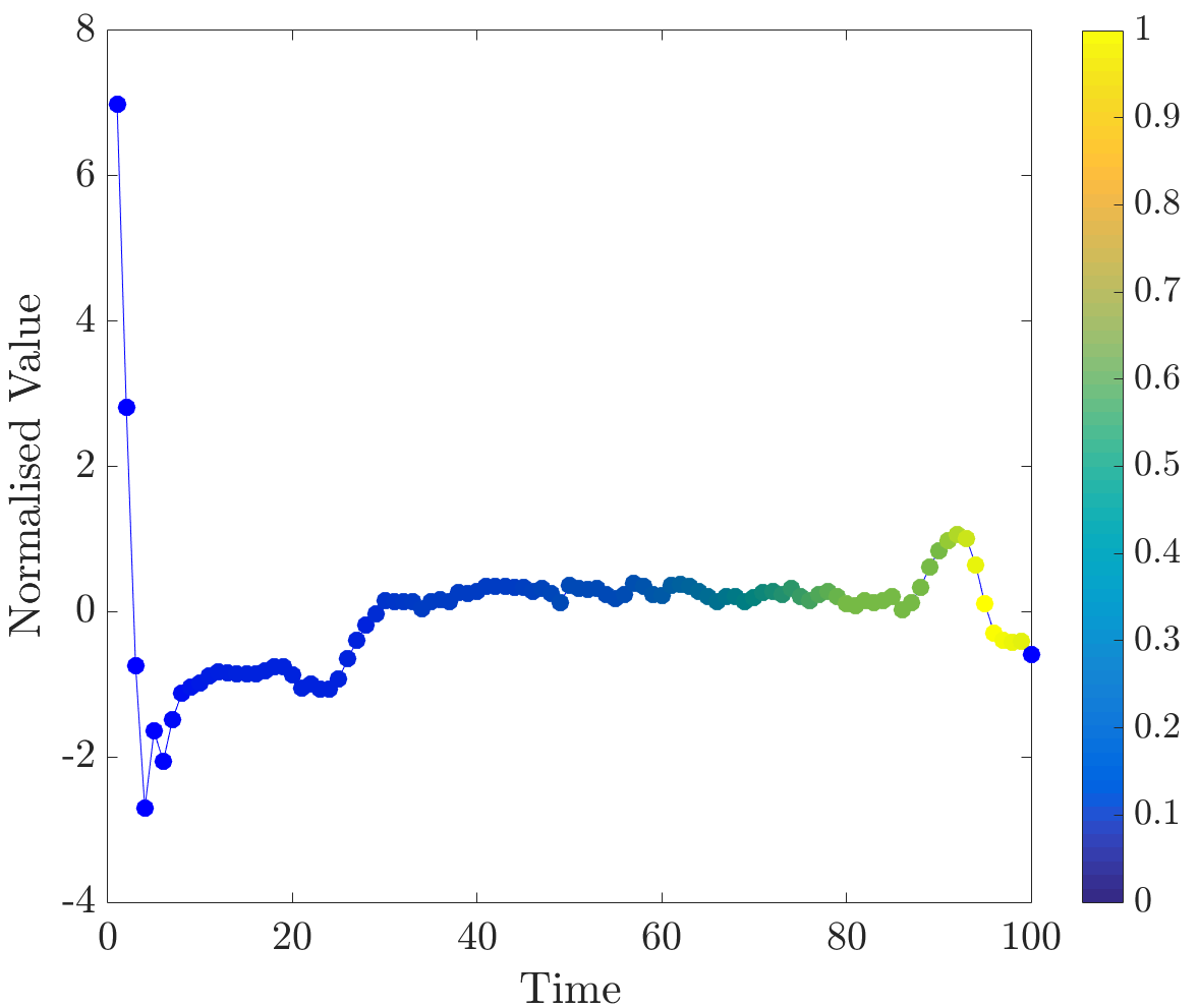 Figure 2
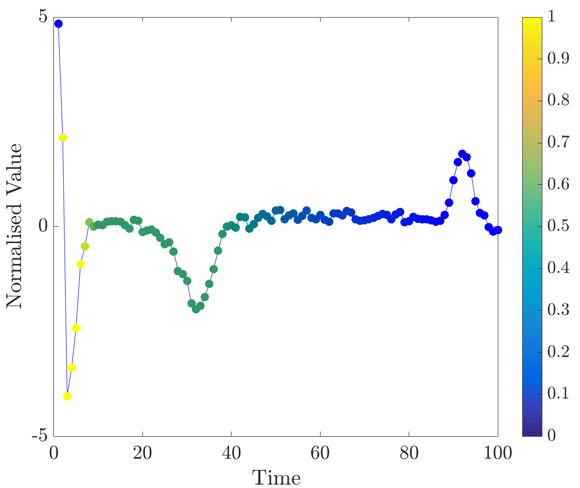 Figure 3
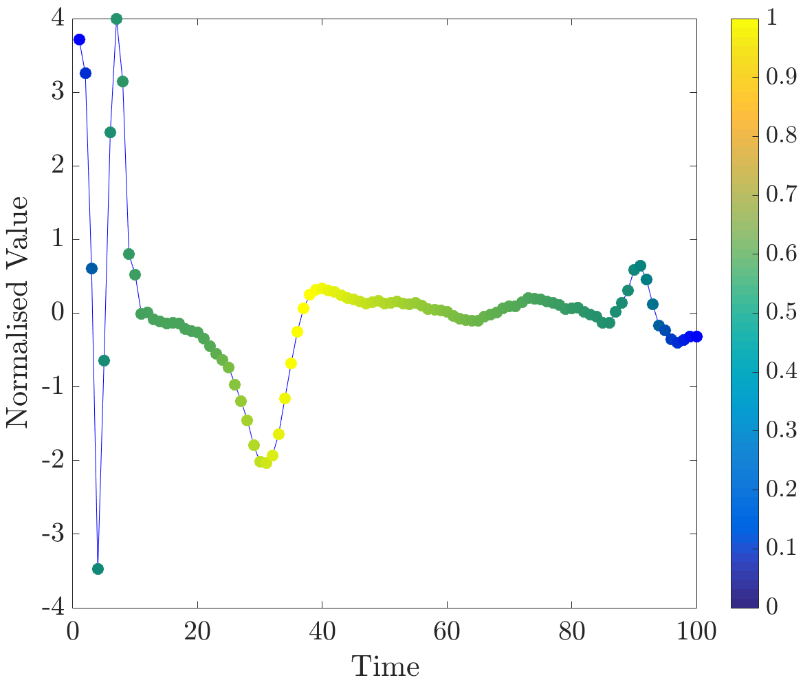 Figure 4
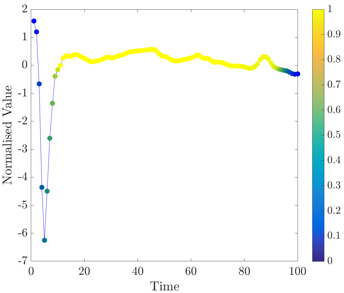 Figure 5
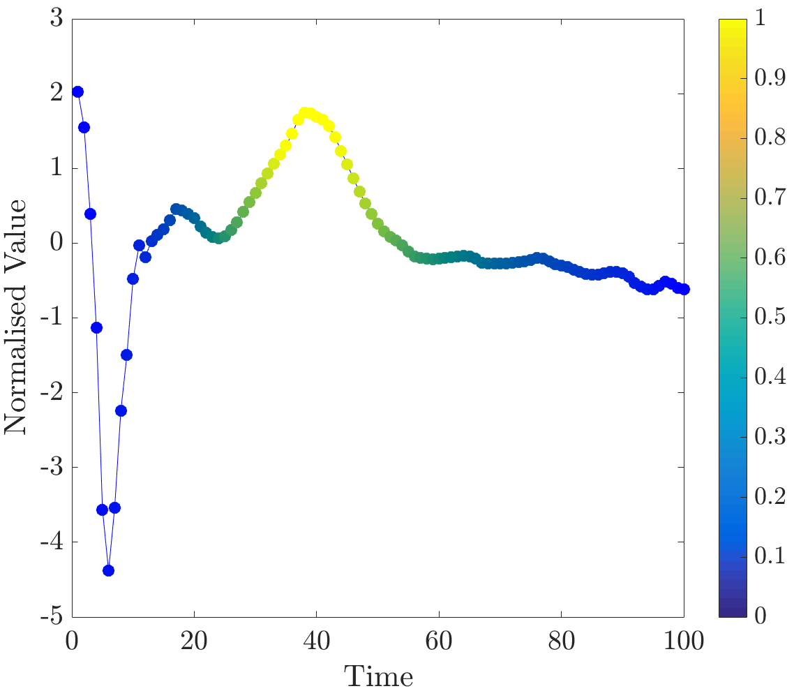 Figure 6
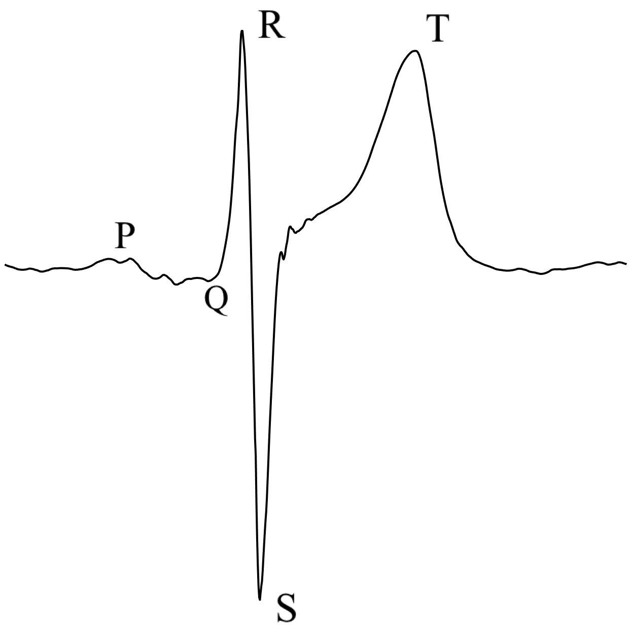 Figure 7
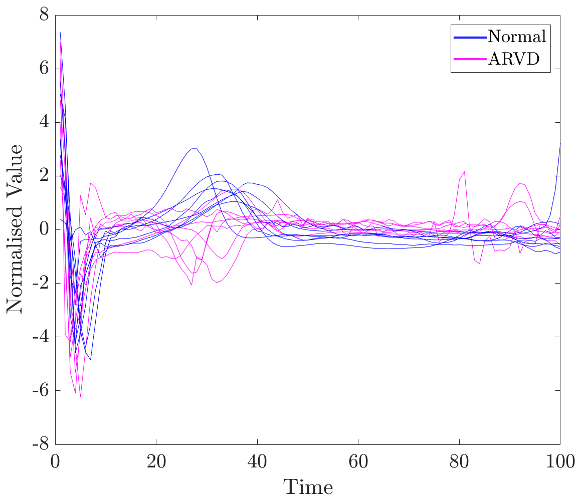 Figure 8
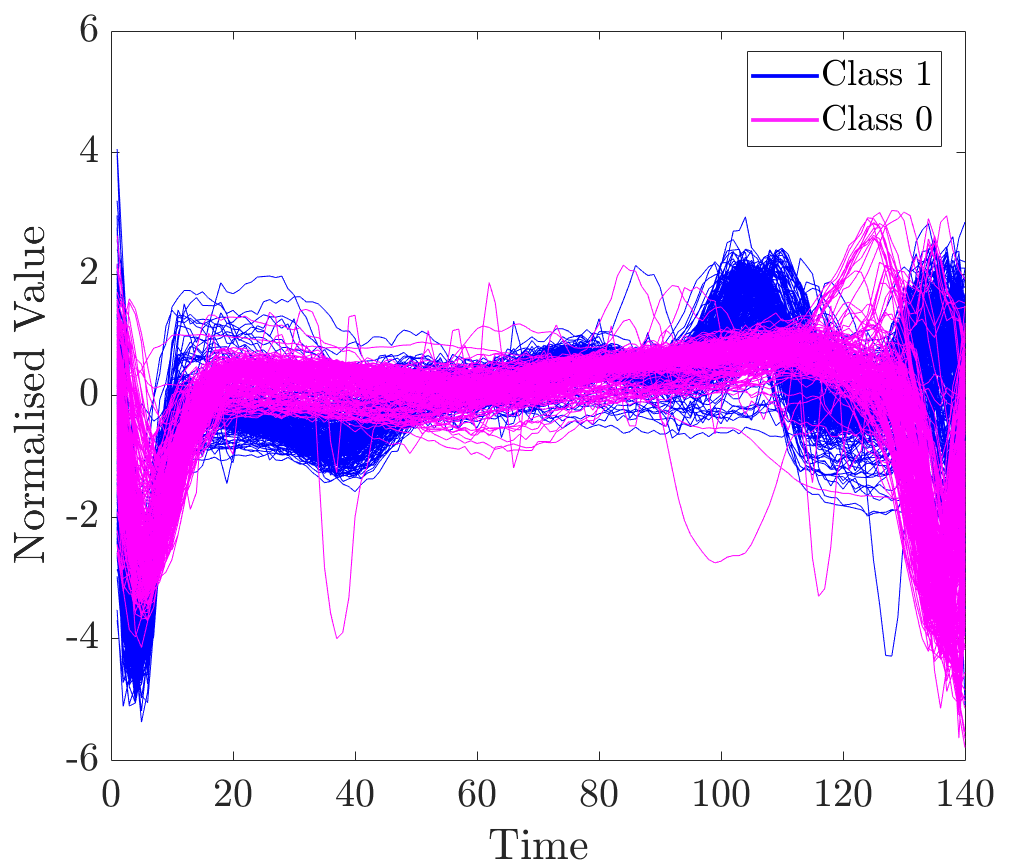 Figure 9
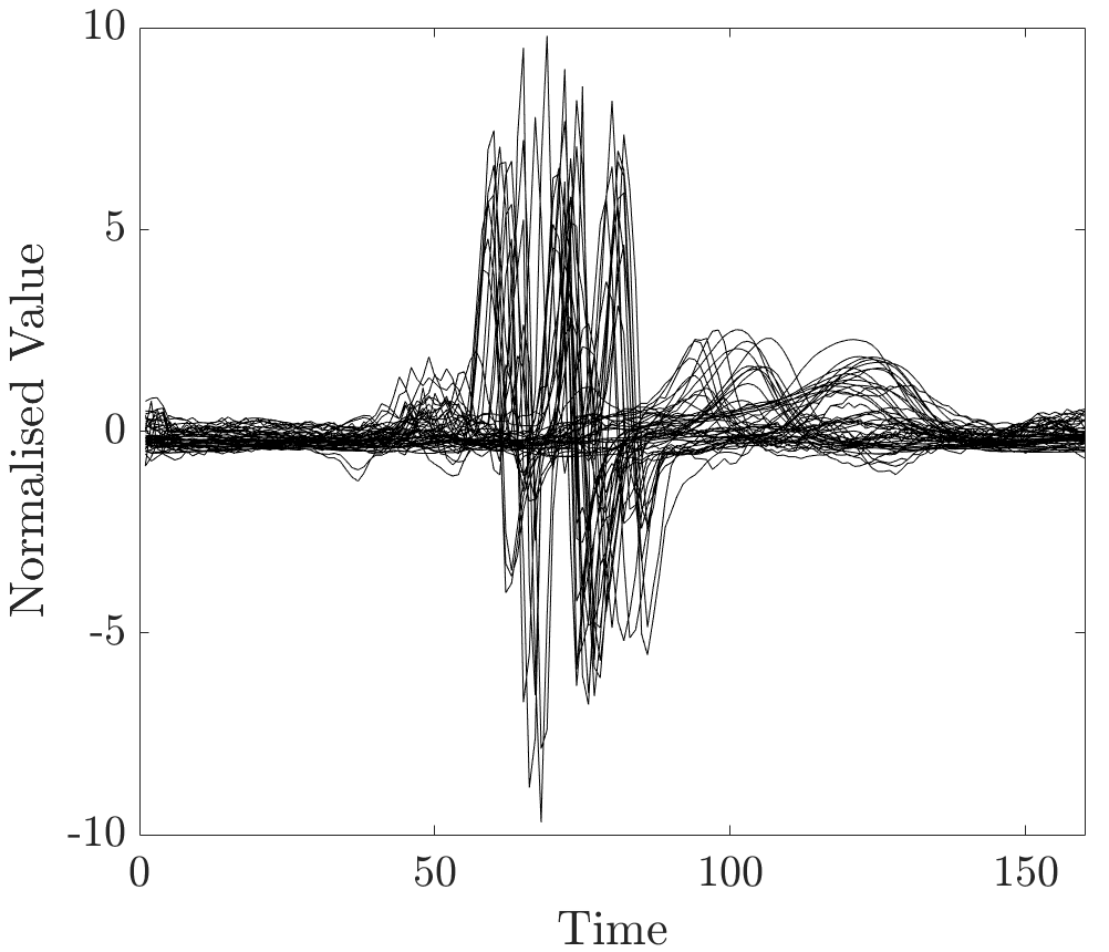 Figure 10
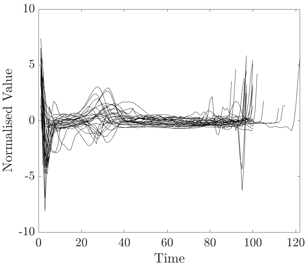 Figure 11
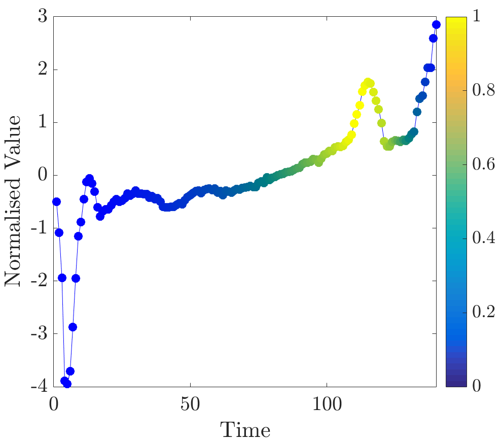 Figure 12
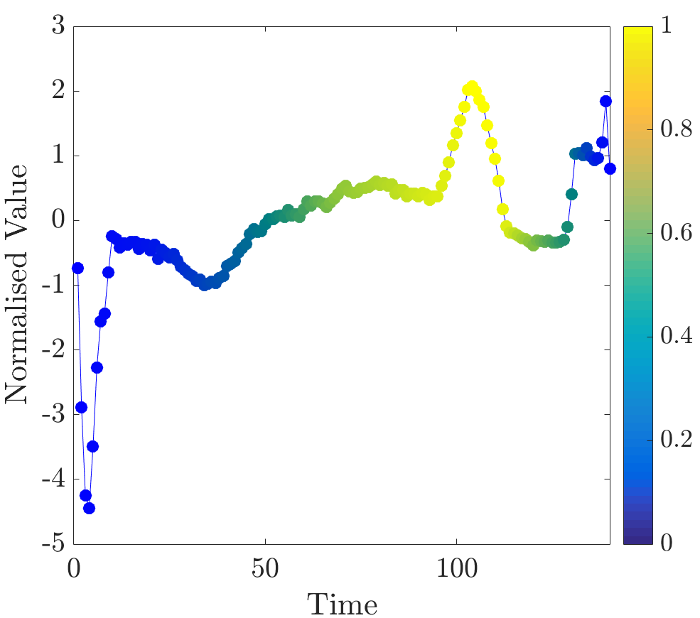 Figure 13
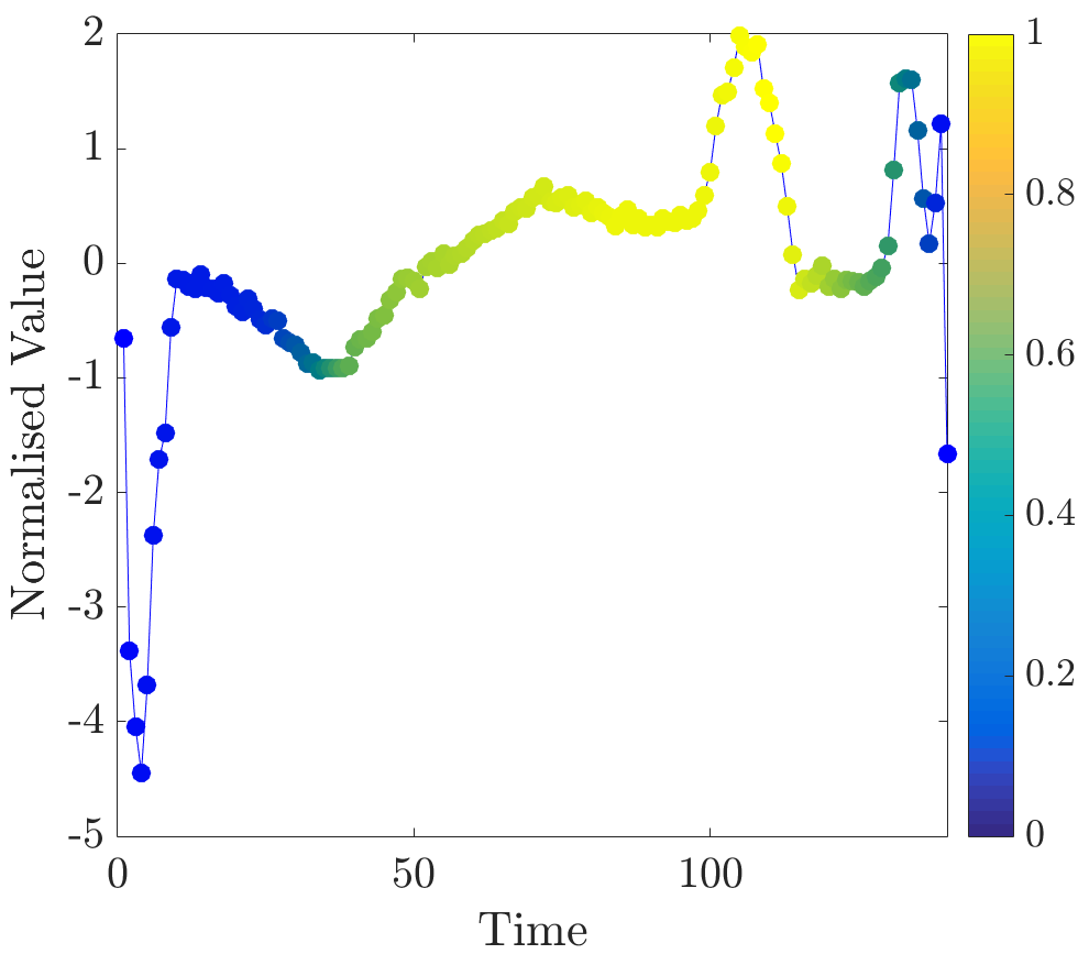 Figure 14
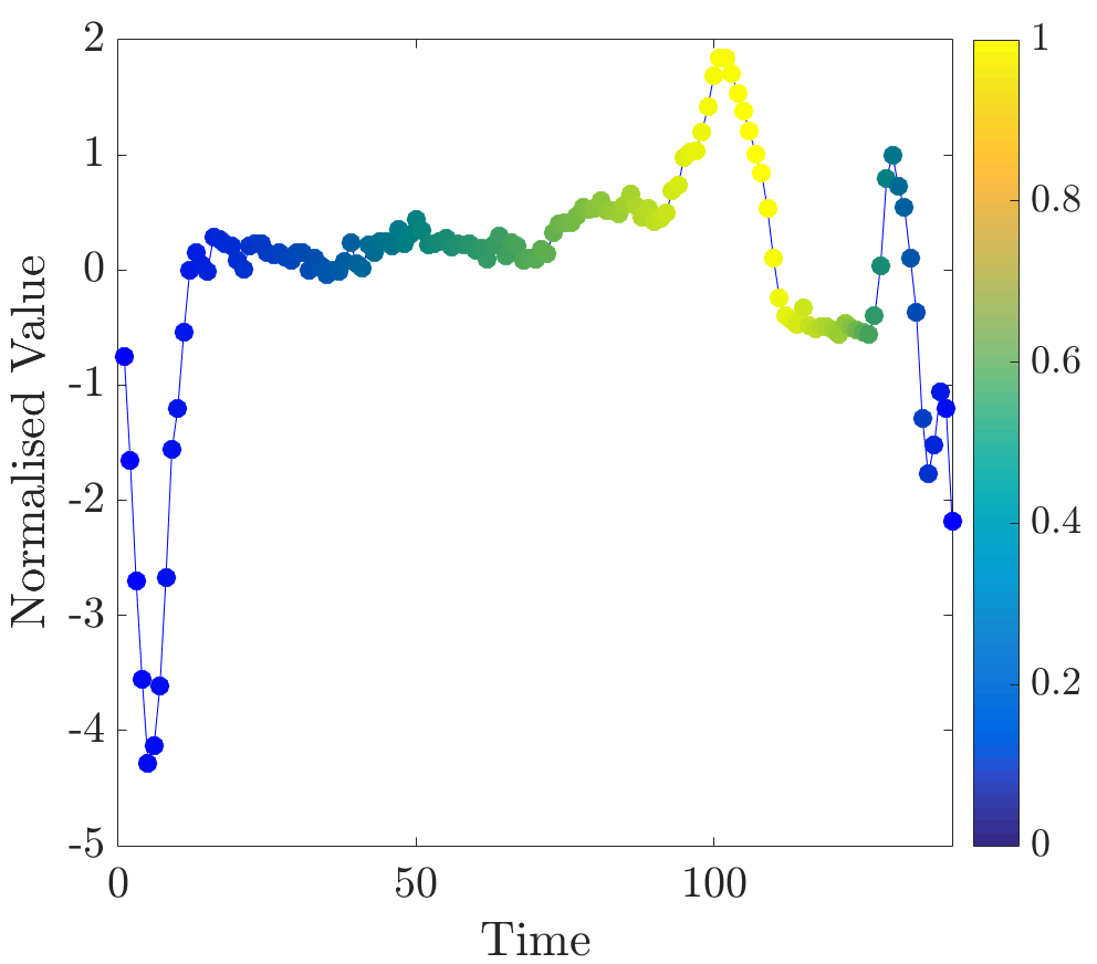 Figure 15
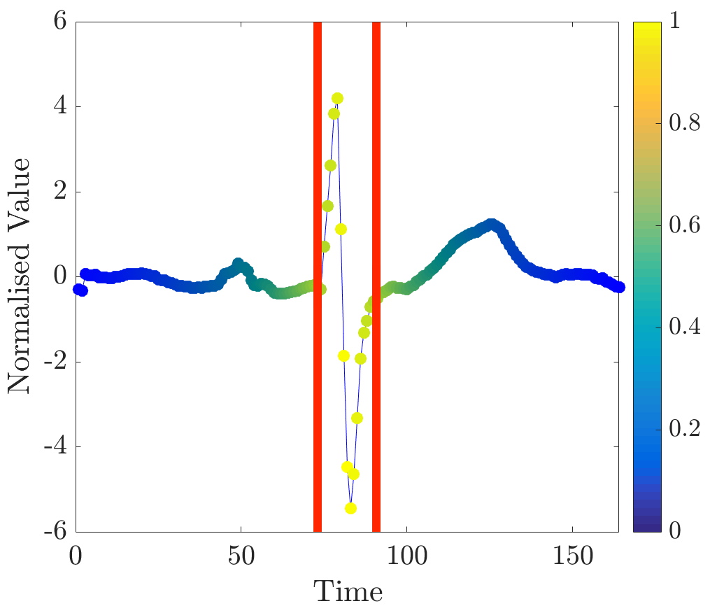 Figure 16
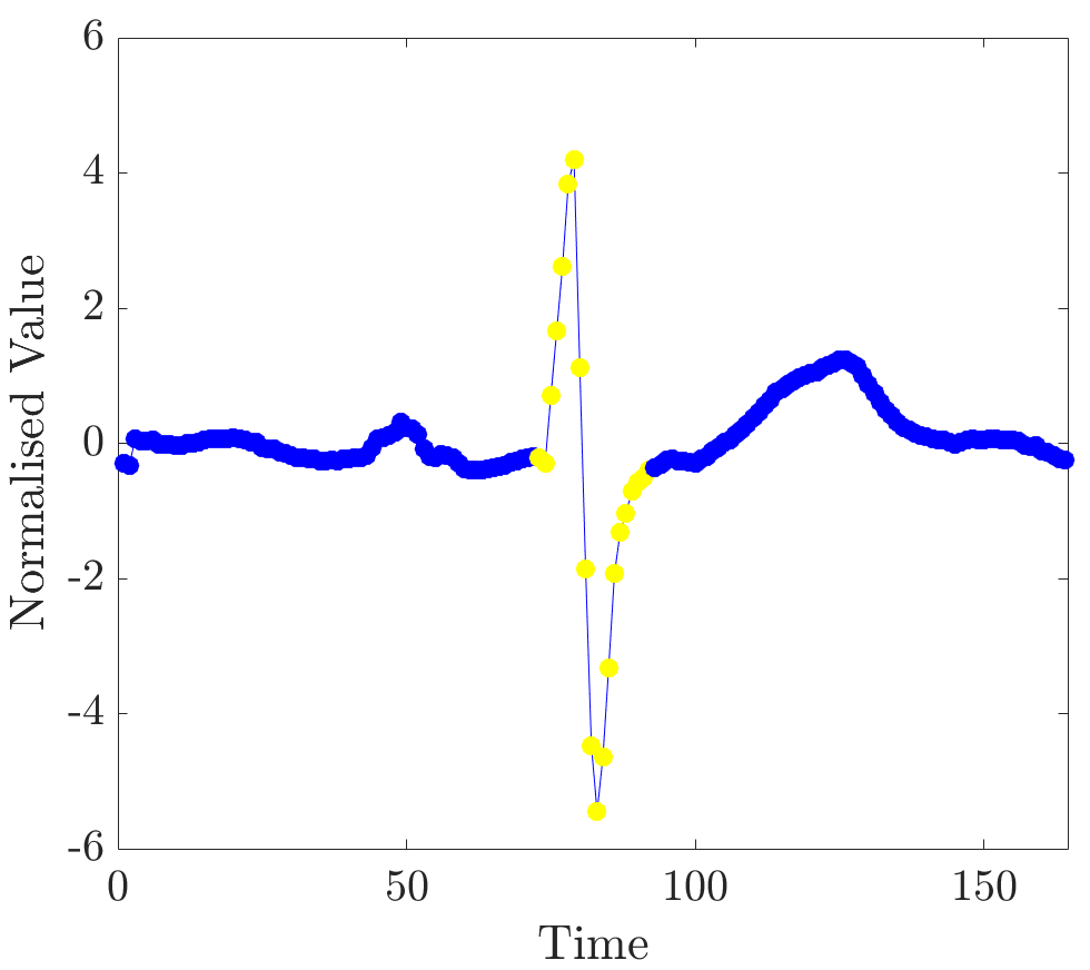 Figure 17
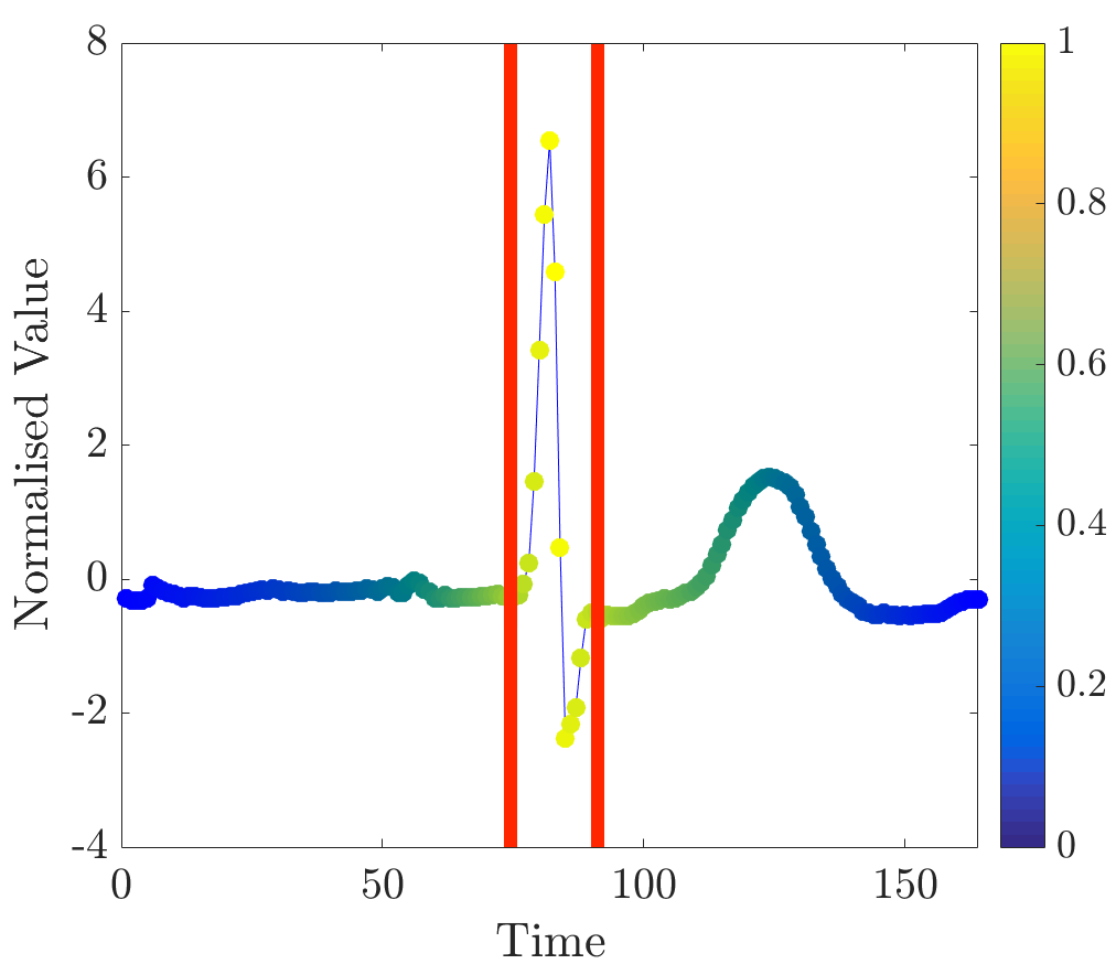 Figure 18
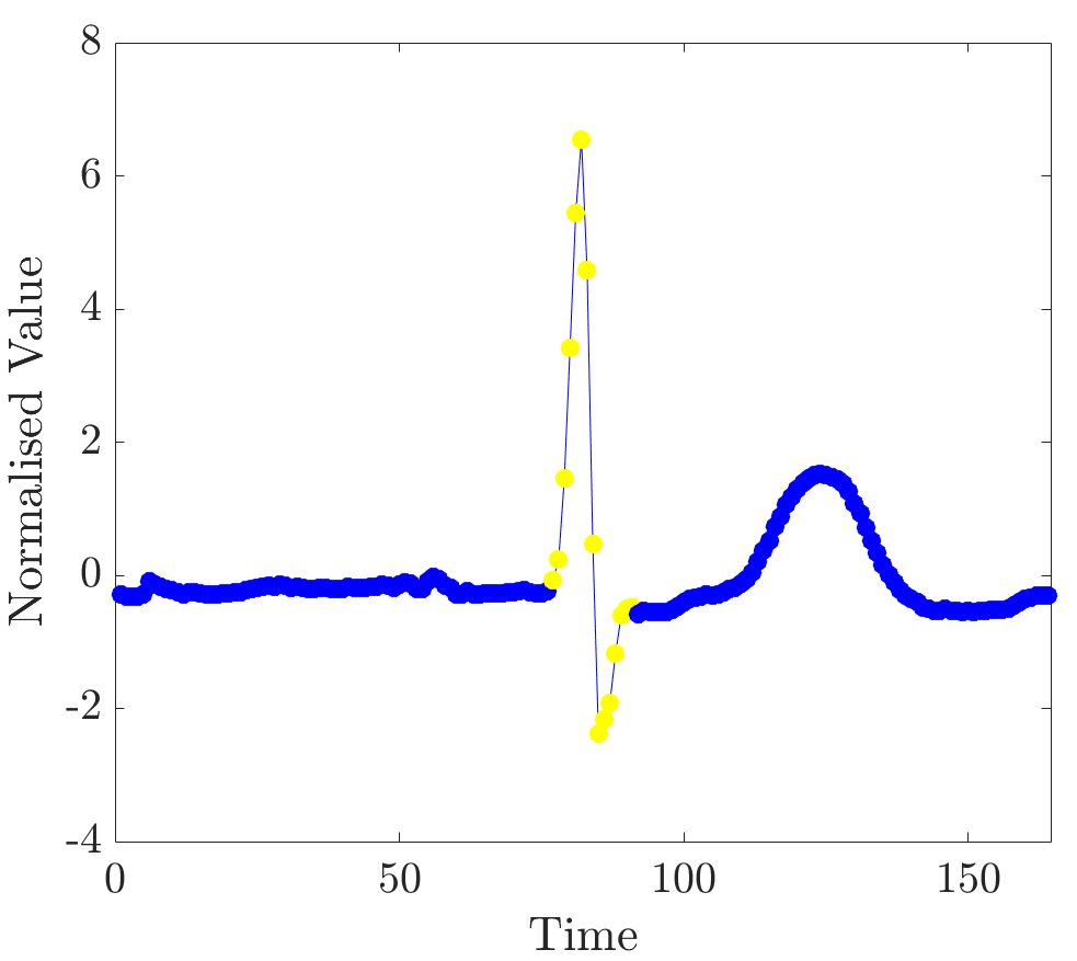 Figure 19
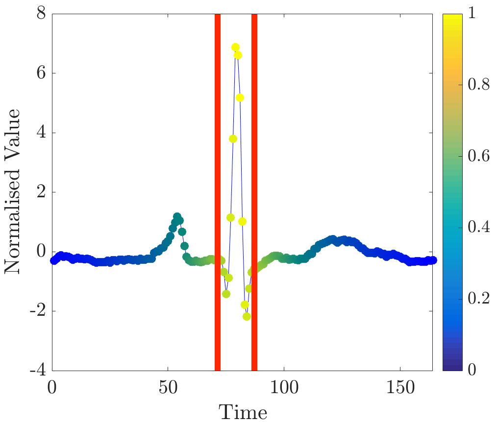 Figure 20
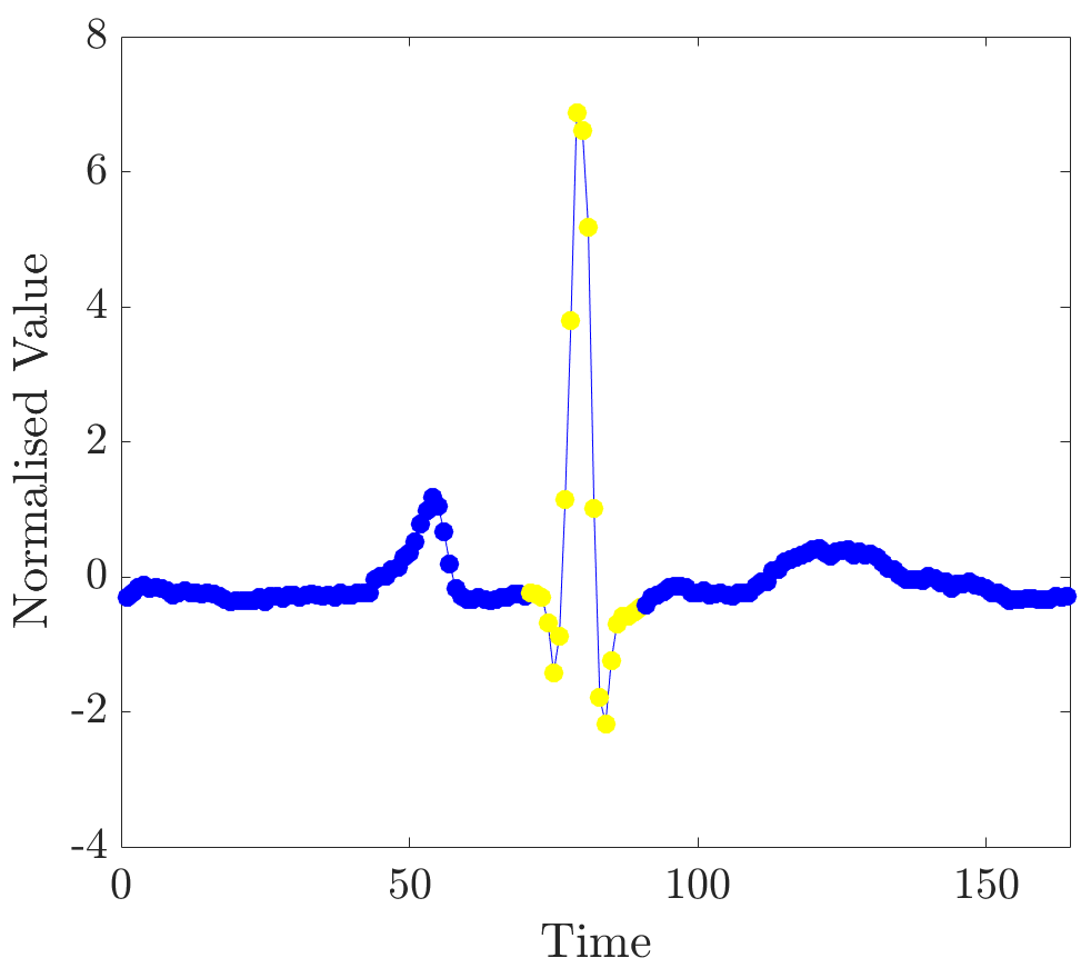 Figure 21
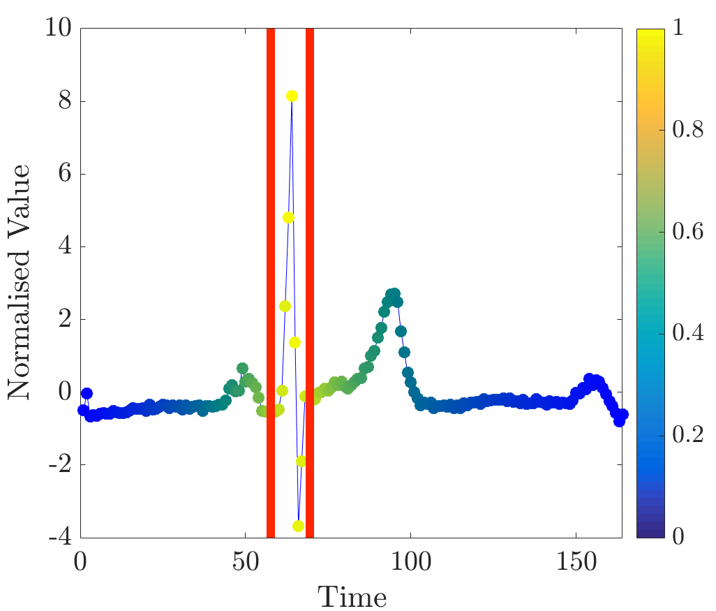 Figure 22
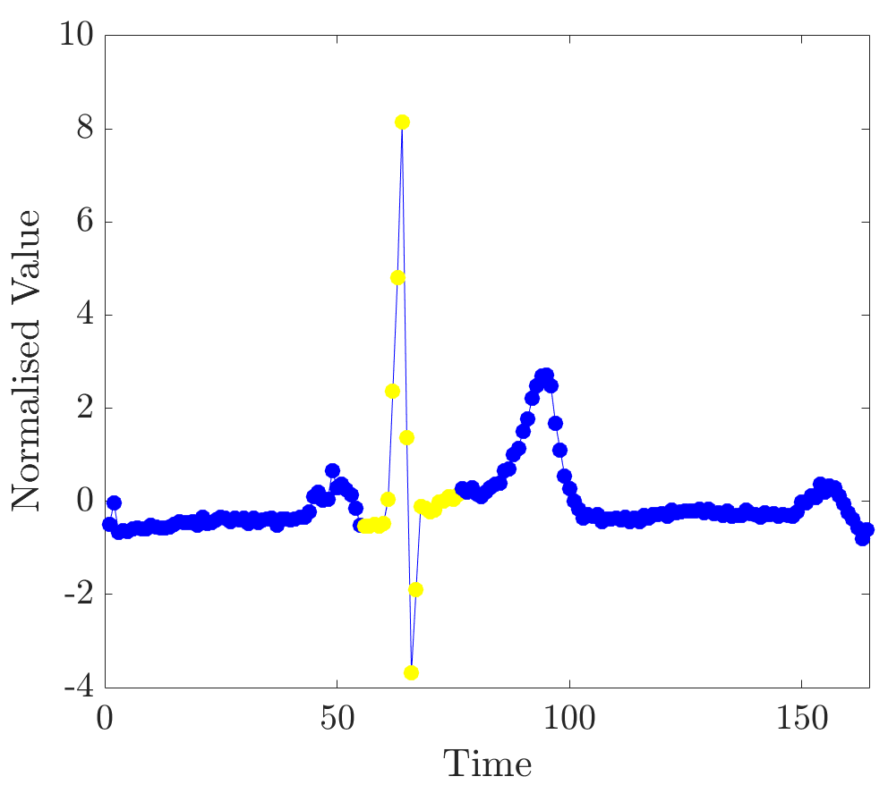 Figure 23
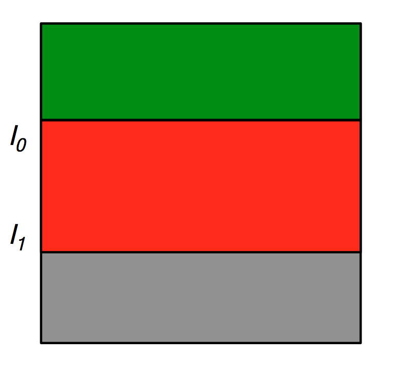 Figure 24
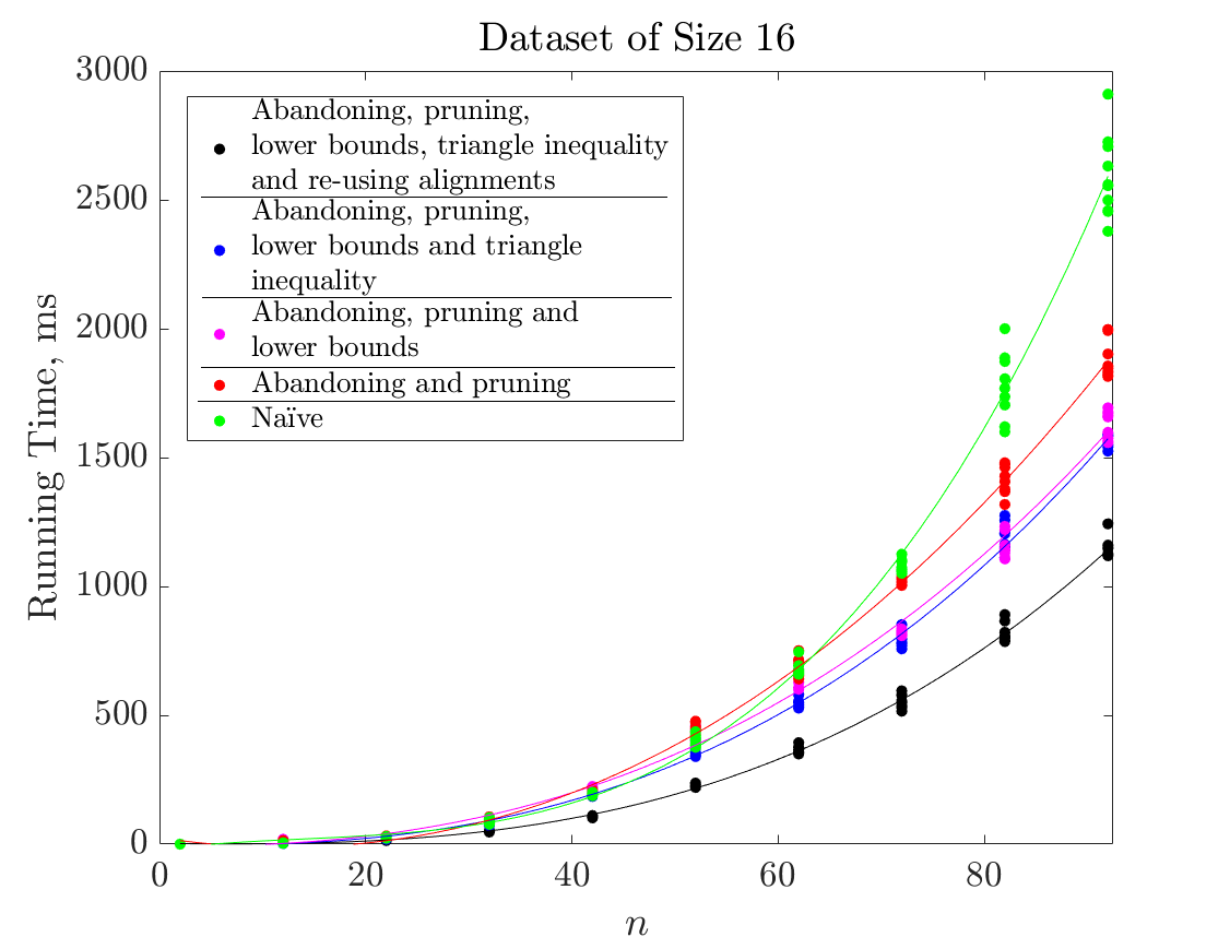 Figure 25
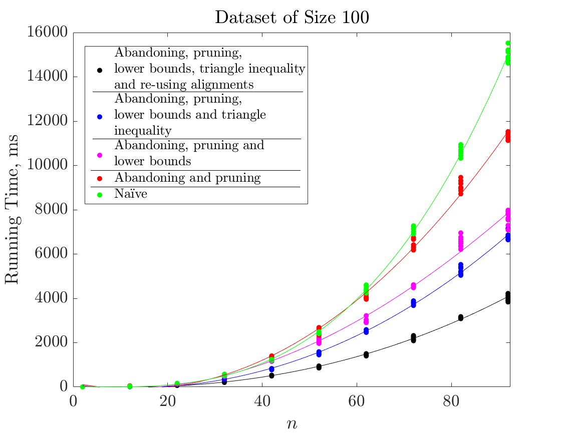 Figure 26
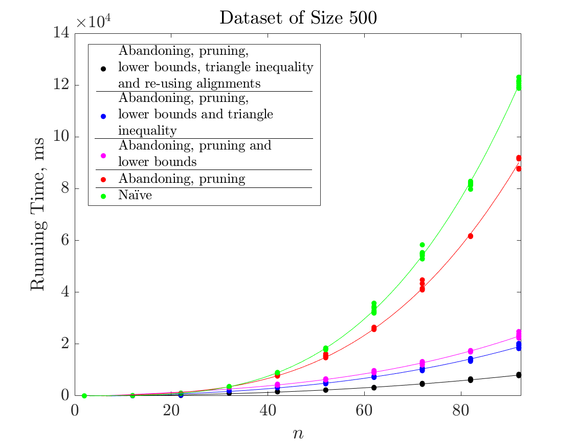 Figure 27
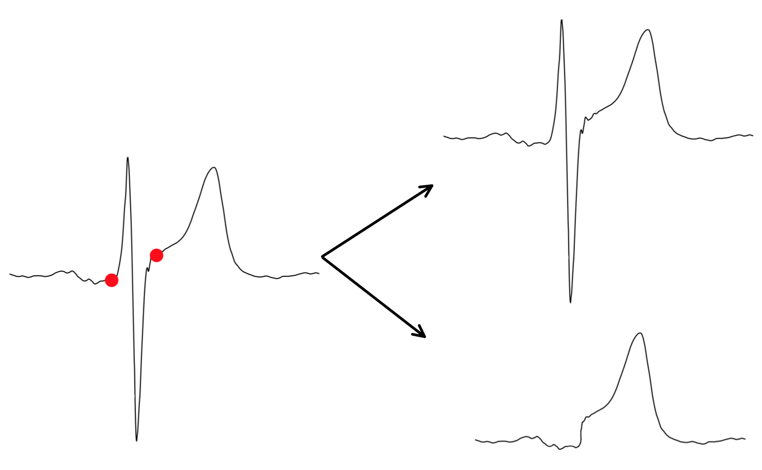 Figure 28
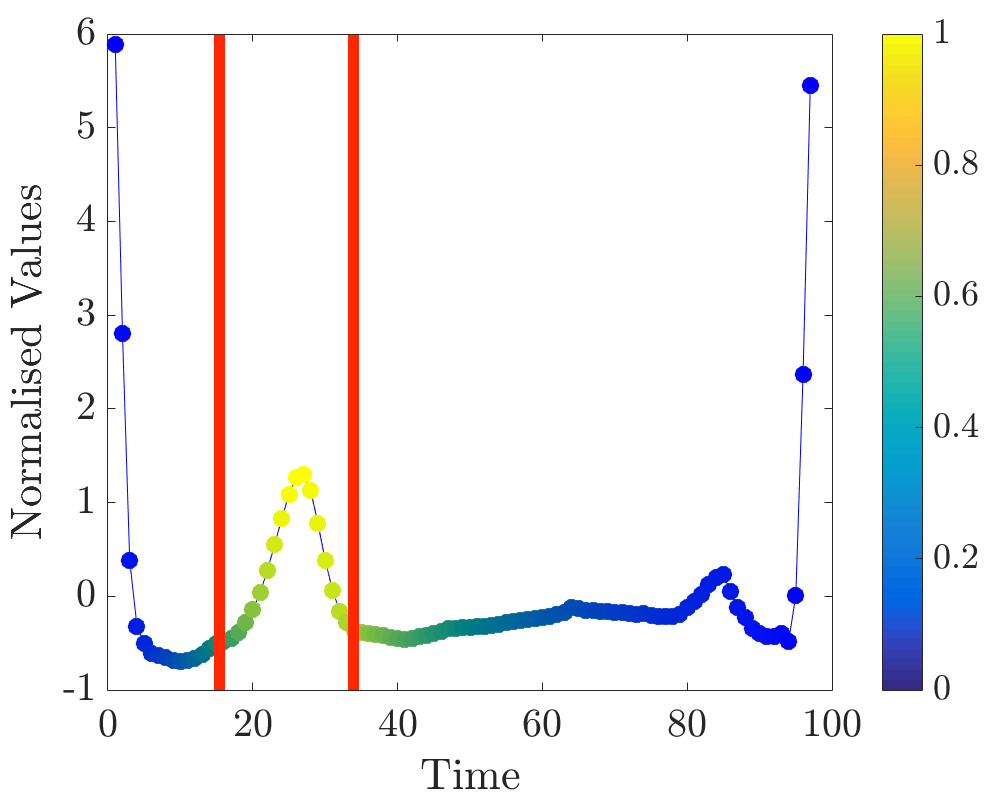 Figure 29
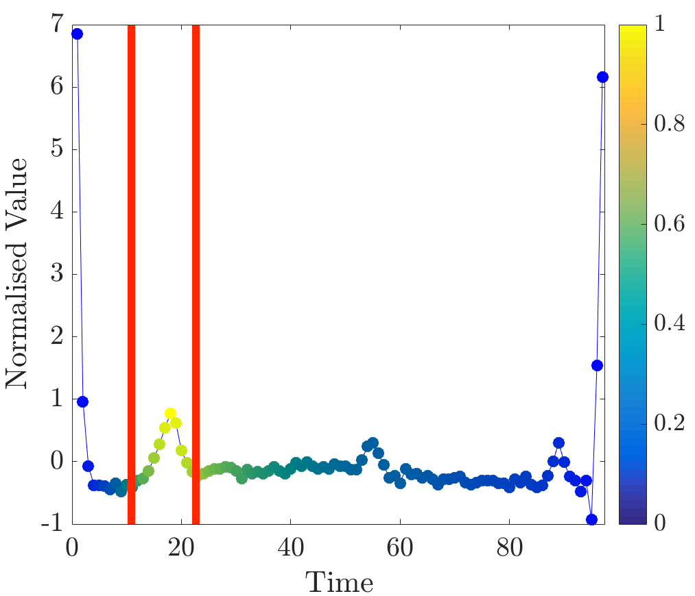 Figure 30
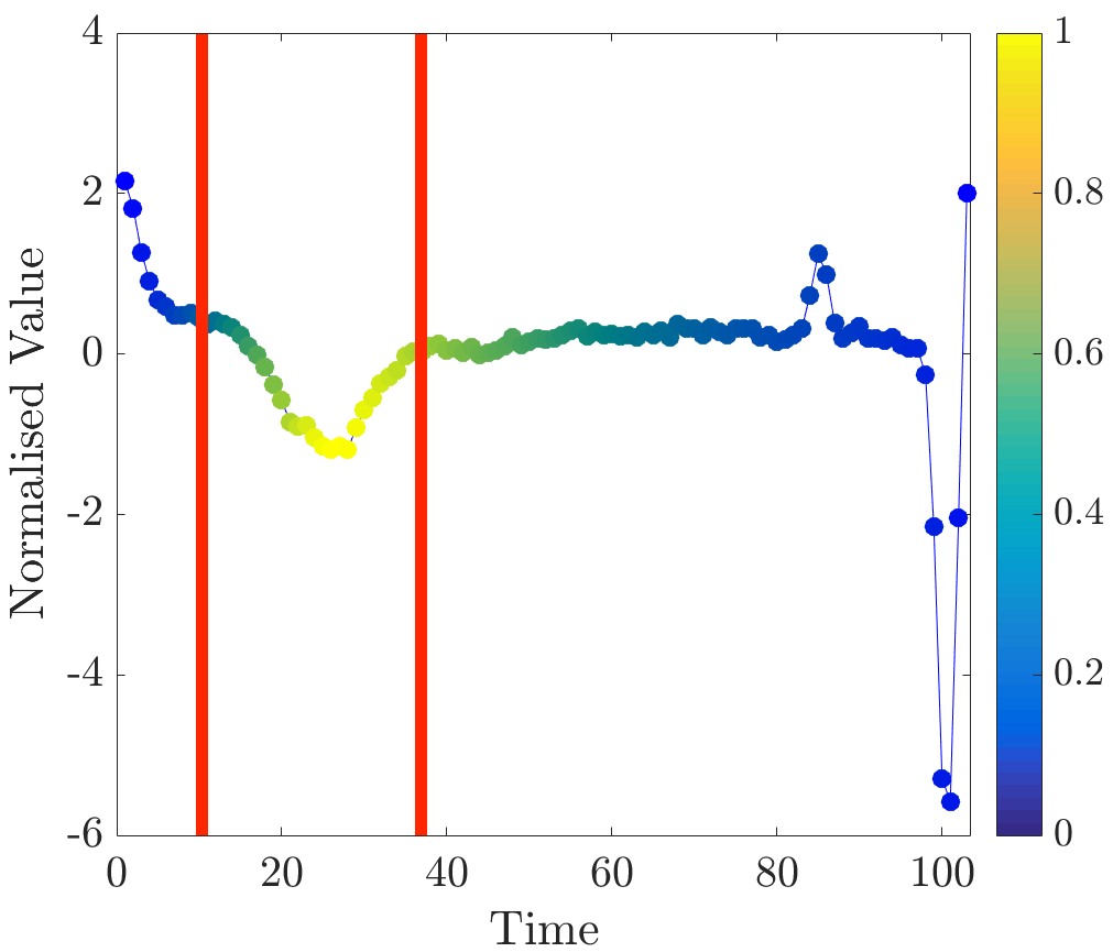 Figure 31
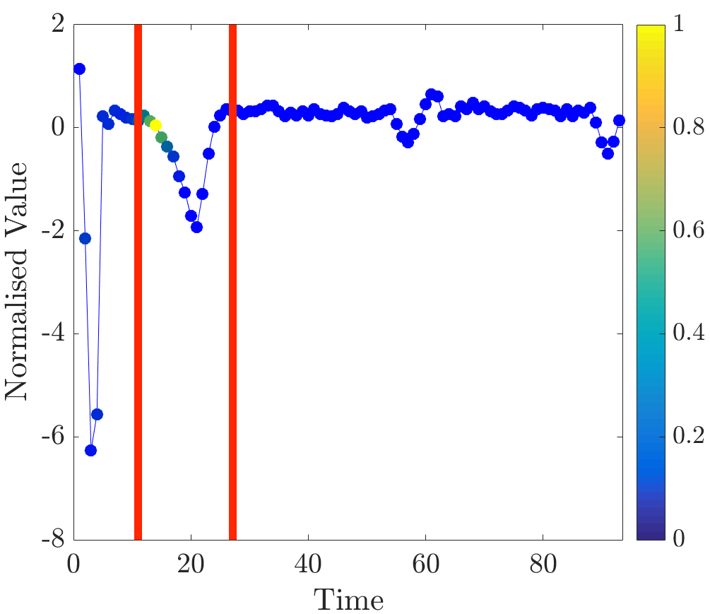 Figure 32
 Figure 33
 Figure 34
 Figure 35
Peer Reviews
No public reviews on file for this paper yet. If you reviewed it on a platform where reviews are public (OpenReview, ICLR, NeurIPS, ICML), you can paste yours below so the community can read it here.
Videos
No videos yet. Explain this paper in a talk, walkthrough, or lecture? Add one.
Taxonomy
TopicsTime Series Analysis and Forecasting · Complex Systems and Time Series Analysis · Anomaly Detection Techniques and Applications
MethodsDynamic Time Warping
Discovery of Important Subsequences in Electrocardiogram Beats Using the Nearest Neighbour Algorithm
Ričards Marcinkevičs, Steven Kelk, Carlo Galuzzi and Berthold Stegemann R. Marcinkevičs, S. Kelk and C. Galuzzi are with the Deparment of Data Science and Knowledge and Engineering (DKE), Maastricht University, P.O. Box 616, 6200 MD Maastricht, The Netherlands. B. Stegemann is with Bakken Research Center (BRC), Medtronic Plc, Maastricht, the Netherlands. S. Kelk is corresponding author, e-mail: [email protected]
Abstract
The classification of time series data is a well-studied problem with numerous practical applications, such as medical diagnosis and speech recognition. A popular and effective approach is to classify new time series in the same way as their nearest neighbours, whereby proximity is defined using Dynamic Time Warping (DTW) distance, a measure analogous to sequence alignment in bioinformatics. However, practitioners are not only interested in accurate classification, they are also interested in why a time series is classified a certain way. To this end, we introduce here the problem of finding a minimum length subsequence of a time series, the removal of which changes the outcome of the classification under the nearest neighbour algorithm with DTW distance. Informally, such a subsequence is expected to be relevant for the classification and can be helpful for practitioners in interpreting the outcome. We describe a simple but optimized implementation for detecting these subsequences and define an accompanying measure to quantify the relevance of every time point in the time series for the classification. In tests on electrocardiogram data we show that the algorithm allows discovery of important subsequences and can be helpful in detecting abnormalities in cardiac rhythms distinguishing sick from healthy patients.
Index Terms:
Time series analysis, classification algorithms, dynamic time warping, algorithmic transparency, dynamic programming, feature discovery.
1 Introduction
Physiological signals are crucial in disease assessment and management. Signals recorded by a digital device, such as a heart monitor, can be represented as time series i.e. measurements performed at regular, discrete time intervals. The automated classification of time series into discrete classes is a natural task. For example, cardiologists might want to draw on computational analysis of electrocardiogram (ECG) data to determine whether a patient has heart problems. Many different approaches have been proposed in the literature for time series classification [1, 2, 3, 4, 5]. Among those the nearest neighbour (NN) algorithm with Dynamic Time Warping (DTW) distance [6] still outperforms several more recent techniques in terms of the accuracy of classification [7]. Essentially this algorithm classifies a newly observed (unlabelled) time series by looking at its nearest neighbours in a set of previously classified (labelled) time series, and taking a majority vote. DTW distance is used to measure proximity and is similar in spirit to sequence alignment on genomic data (formal definitions will follow). Despite the fact that current research largely focuses on designing accurate classifiers, which under experimental conditions typically place unlabelled time series in the correct class, we might not always be interested only in the accuracy. In particular, we might also wish to know why an instance was classified in a particular way. Such questions become especially pertinent in light of new (European) regulations demanding transparency in computer-supported decision-making [8].
Here we propose to answer the why? question by studying modifications (i.e. perturbations) of the input sufficient to alter the classification outcome. In particular, leveraging a parsimony perspective, it may be useful to find a simplest such modification. We formalise this as follows. Given a labelled dataset of time series with a discrete set of classes and an unlabelled instance , find a minimum length subsequence of the instance the removal of which changes the outcome of its classification under the nearest neighbour algorithm with DTW distance. Observe that, if , the number of subsequences of the time series is . Therefore, a naïve search through the space of all candidate solutions is impractical. The problem can be simplified by considering only contiguous subsequences of which there are . In this article we consider only this simplified version of the problem, but as we shall demonstrate this is still powerful enough to detect interesting features in real-world data.
The structure of this article is as follows. In Section 2 we provide background information on time series data, the nearest neighbour algorithm, DTW distance and also some basics on interpreting electrocardiogram (ECG) data (which forms the core of our experimental study). We also explain how our approach differs from other approaches in the literature.
In Section 3 we describe our approach for solving the problem, which consists of the natural subsequence search algorithm augmented with a number of enhancements to reduce the running time, such as efficient re-use of the DTW dynamic programming table and pruning. We also introduce a measure for assessing the relevance of points in the time series data: informally, how frequently they occur in minimum modifying subsequences. Section 4 presents and interprets the results of our experiments on ECG data. The intuition is that minimum modifying subsequences will potentially contain ECG waveform segments and points which are relevant to the underlying diagnostic problem. This in turn may help to interpret the classification result for specialists and even to discover new knowledge about the morphology of the ECG under certain diseases. The results are encouraging and support this intuition; see Figure 1 which is reproduced from our experimental section. Another set of experiments we conduct demonstrates that our method is not only useful for interpretation and discovery of important subsequences, but also (when used ‘backwards’) as an instrument for detecting and locating known features. Finally, in Section 5 we reflect on our work and consider solution perspectives for the non-contiguous version of the problem.
2 Preliminaries
2.1 Time Series Data
Electrocardiograms and many other signals can naturally be represented by time series. A time series with points, equally spaced in time, is described by a sequence of values , where refers to the value measured at the -th time point. Based on this simple representation, signals can be compared, clustered or classified [10]. In particular, comparison can be performed using some (dis-)similarity measure, for example, Euclidean distance. For a good overview of time series data mining, see [10] and [11].
2.2 The Nearest Neighbour Algorithm and Search
The -nearest neighbour (-NN) algorithm is perhaps the simplest instance-based classification technique and has been well-studied in the machine learning literature [12, 13, 14]. Given a dataset of labelled training instances and an unobserved instance to be classified, this algorithm returns the label that is most common among training instances closest to the unobserved instance, according to some distance function (and breaking ties in some systematic way) [15]. In this article, to clarify the exposition, we focus on the case and assume only two classes; however, all of the methods presented can be easily generalised to non-binary classification with .
The NN algorithm includes solving an optimisation problem known as nearest neighbour searching [16], formally defined in the following way. Given set of instances, distance function and query instance , we need to find instance , which will minimise . Depending on the distance function various refinements can be made to accelerate identification of this minimum [16, 17].
2.3 Dynamic Time Warping
A viable distance function for the NN algorithm is Dynamic Time Warping (DTW) distance. This a distance measure for time series data, used in a wide range of domains [18]. It is evaluated based on a least ‘cost’ alignment between two time series. Although the details differ it is analogous to the task of pairwise sequence alignment of DNA sequences encountered in bioinformatics.
The DTW distance between two time series and , and points long, respectively, can be defined recursively as follows [19]:
[TABLE]
where is the empty series; denotes a local distance function (we assume ); and stands for the contiguous subsequence of time series beginning in the -th time point and ending with the -th. Note that and do not need to be equal.
Based on the recurrence relation above DTW distance can be computed by dynamic programming. This aligns the two sequences by finding an optimal warping path through the grid of distances [6, 20]. The running time complexity of the standard implementation is [19, 21].
The optimal warping path satisfies monotonicity and continuity constraints [6], i.e. aligned points are ordered monotonically w.r.t. time and the steps of the path are confined to neighbouring points in the grid. Additionally, a warping window constraint can be imposed [6] by allowing warping paths only within a certain window.
In order to avoid computationally expensive evaluations of the DTW distance during NN search, quickly computable lower bounding functions are often utilized. If the lower bound is already too large the time series cannot possibly be one of the nearest neighbours and can be immediately excluded. Several lower bounds have been proposed in the literature [19, 22, 23]. It is also important to mention that fast (linear in time) approximations to the DTW distance exist. For instance, the FastDTW algorithm approximates the distance by computing the alignment between down-sampled time series [24].
2.4 Electrocardiograms
We have tested our method on electrocardiogram datasets. The surface electrocardiogram (ECG or EKG) quantifies the electrical potential between points on the body [25]. It is recorded by placing electrodes (leads) on the body in various sites [25]. This technique is widely used for the measurement of heart activity and can be utilized in the diagnosis and management of various pathologies.
An ECG signal can be characterised by various relevant points, segments and waves. Figure 2 depicts a beat from an ECG of a healthy person; and waves, as well as points , and are marked in the plot. All of these landmarks have a physiological meaning in terms of the cardiac cycle [25].
It is important to note that the morphology of the beats can vary dependending on the electrode position and on the disorders that the heart suffers from [25].
2.5 Related work
The classification of time series requires a tailored approach due to the temporal ordering of its datapoints. Many algorithms have been proposed to classify time series data. Broadly speaking there are two major approaches to the problem: feature- and distance-based [26]. The former amounts to extracting a set of features from raw time series prior to training a classifier [26], examples of simple features are averages and standard deviations of time series intervals. A feature-based approach to classification is discussed in [4], where time series are classified by a support vector machine (SVM) trained on predicate features extracted from intervals. The latter approach, on the other hand, quantifies dissimilarities between time series (raw or transformed) and then usually applies an instance-based classification algorithm [26]. For example, the -nearest neighbours algorithm with weighted DTW distance, proposed in [1], is a case of distance-based classification. Most of the approaches, distance- or feature-based, provide little explanatory power. While literature about training accurate classifiers and understanding them is abundant, the problem of interpreting individual classification outcomes and discovering important intervals within time series is addressed less frequently.
To the best of our knowledge our approach has not been described in the literature before. However, two primitives from the time series data mining literature exhibit some (superficial) similarity to our approach. The problem of finding a time series discord [27], the most ‘unusual’ subsequence, is relevant, because it targets the discovery of important time series segments. A discord is formally defined as a contiguous subsequence of a time series, which has a maximum distance to its closest non-self match i.e. another subsequence that does not overlap with it. Discords were demonstrated to be useful in anomaly detection in various sensor time series, such as ECGs. Other relevant time series primitives are shapelets [28]. A shapelet can be intuitively viewed as a time series subsequence that is identified as being representative of an entire class in a two-class dataset. For the formal definition of shapelets the reader is referred to [28]. Shapelets can be used for a fast and interpretable classification.
Both of these primitives involve the analysis of subsequences in time series data and in that sense resemble our approach. However, neither involves the NN algorithm or the DTW distance (explicitly). Moreover, these primitives are not intended for interpreting classification outcomes at the level of individual time series. Discord is useful for detecting anomalies within a single time series (i.e. it does not consider other time series) and shapelet analysis can be used to identify general characteristics of a class - but it does not act at the level of an individual time series. For this reason our approach is not directly comparable to these earlier approaches and we do not consider them in our experiments.
3 Method
As mentioned before, there are only many contiguous subsequences of a time series. Therefore, it is possible to search through all of them exhaustively for reasonable-sized . Algorithm 1 contains the conceptual pseudocode for the naïve search, for , which iteratively considers subsequences of increasing lengths.
Herein, operator “” denotes concatenation of sequences. Note, that in this search subsequences containing end-points of are not considered; we make the assumption, for the sake of convenience, that the end-points may not be removed. This algorithm is merely a naïve search procedure and can be further optimised.
As can be seen, the essence of the search is simply to consider all subsequences of increasing length and to perform NN classification each time. It is difficult to construct efficient data structures for NN searching under the DTW distance, because it is non-metric and the assumptions made by many other algorithms (in particular: that the triangle inequality holds) are not valid here [16, 17]. Moreover, many tight lower bounding functions on the distance proposed in the literature are also not applicable, because they assume that the two time aligned series are of the same length [19, 22, 23]. Due to the deletion of subsequences this assumption also does not hold in our case. For these reasons we have elected to use the standard, linear NN search. Nevertheless there are several practical improvements which can be applied; many of them are tailored to our specific, DTW-based deletion approach and are thus not implied by more general techniques for NN search optimization. Namely, we enhanced the procedure by
- •
early abandoning [18] and pruning [29] of DTW distance computations;
- •
re-using old DTW alignments in new distance computations and lower bounds;
- •
repairing the DTW distance function [16] to make it satisfy the triangle inequality, from which lower bounds can be derived.
Early abandoning and pruning distance computations as well as repairing distance functions has been discussed in the literature before, and we refer the reader to [16, 18, 29] for more details. Nevertheless, re-using DTW alignments is novel to this problem and is explained further.
When initially classifying an unobserved time series , DTW alignments between and training instances from dataset have to be computed. These alignments can be re-used further. We demonstrate that lower bounds on distances between a modified time series and training instances can be inferred from these alignments. Moreover, they can be re-used when computing new alignments, if needed.
Let denote a times series that resulted from a modification of . was constructed by removing a contiguous subsequence from , such that the left-most point of this subsequence is at index and the right-most is at index . Consider the DTW alignments between and some training instance and between and . By construction, dynamic programming tables for these alignments, and , respectively, are identical from row [math] to row inclusively. This is schematically illustrated in Figure 3.
Based on this invariance, for every time series in the dataset, a lower bound on its distance to the modified time series can be derived from its initial alignment with . If both and are placed close to the left end-point of , then this lower bound will not be very tight. In that case a tighter lower bound may be derived in the same manner from the alignment between and , which are the reversals of and respectively.
What is the utility of the aforementioned lower bounds? They can be used to prune the standard, linear nearest neighbour search and avoid expensive DTW distance evaluations. In particular, given a modified time series , some from the training set and upper bound on the distance to the NN of , can be pruned in the NN search if where is a lower bound on .
Apart from computing lower bounds on distances, the initial alignments can be stored in memory entirely, to re-use the DP tables for modified time series. In general, if a subsequence from to is removed from , then the computations of the alignment between and any time series in the training set can be started from row based on row of the initial alignment between and the training instance. In practice this can speed up the algorithm considerably at the cost of increasing the space complexity, because complete dynamic programming tables have to be stored.
3.1 Relevance of Time Points
A minimum length subsequence the removal of which changes the outcome of classification is expected to contain points of the time series that are relevant to the considered classification task. However, we observed that the minimum length subsequence alone often is not sufficiently interpretative. Therefore, we propose a measure that, intuitively, is expected to quantify the relevance of every point in the time series for the classification.
For an unobserved time series , let denote the set of contiguous subsequences, the removal of which changes the outcome of classification of and which contain the -th point of . For every point , relevance is given by
[TABLE]
The relevance value is thus simply the sum of the inverted lengths of subsequences in . Therefore, this measure promotes the points which are contained within many subsequences and, especially, the points which are contained within many short subsequences.
Note, that Algorithm 1 can be easily adjusted to calculate the relevance vector for the input time series. Computing relevance values requires at least as many operations as finding the minimum length subsequence. Moreover, non-minimum length subsequences have to be found as well. The problem can be relaxed by considering only those subsequences which begin at every -th time point or by considering subsequences shorter than a given length; this results in a faster approximation of relevance values.
The relevance measure is expected to provide a visual and informative way for interpreting the classification of individual time series, given some dataset. It can be used to identify time series segments particularly relevant to the considered classification problem.
4 Experiments and Results
In order to verify the designed algorithm and its performance, several experiments were conducted. In this section, we describe the datasets that were used in testing, how the data was pre-processed and, finally, the experiments themselves and their results. Our first experiment in Section 4.2 studies the scalability of our method for computing relevance values. In our second experiment, in Section 4.3, we use our method to interpret classification (through discovery of important subsequences). In the third experiment, Section 4.4, we use our method ‘backwards’ to detect subsequence types that we have identified a priori as being of interest. For all experiments a computer with 2.3GHz quad-core Intel Core i7 CPU and 8Gb memory was used.
4.1 Datasets and Processing
We used several ECG datasets. In particular, two most common classes were taken from the training set of ECG5000 beat dataset, available at the UCR Time Series Classification Archive [30]. Other datasets, obtained from this archive, were CinC_ECG_torso testing set with several classes of ECG beats and two-class ECG500. We also constructed a set of beats from various ECGs available in the PhysioBank databases [31]. Finally, ECG beats from the small dataset of normal subjects and patients diagnosed with arrhythmogenic right ventricular dysplasia (ARVD) [9], kindly provided by Leeds General Infirmary, were used as well.
Prior to running tests, some ECGs were denoised in the MATLAB environment using wden function for automatic signal denoising with wavelets, db4 (Daubechies family) wavelet was applied. After that, if needed, the time series were normalised and down-sampled. For some of the experiments, complexes and waves were labelled manually.
Finally, relevance values were computed for the chosen unobserved time series by the designed algorithm, implemented in Java alongside some important subroutines for (amongst others) the DTW and the NN algorithms.
4.2 Algorithm Scalability
An experiment to test the scalability of the implemented procedure was conducted. The running times for computing relevance values for each time point in unobserved time series of varying lengths () were measured. Measurements were performed for three datasets of different sizes, namely, the set of ARVD beats, ECG500 and ECG5000. Figure 4 contains the plot of running times versus different time series lengths for sets of 16 (4a), 100 (4b) and 500 (4c) instances. Relevance values were computed by different versions of the implemented algorithm (see figure legends for details).
The implemented enhancements (abandoning and pruning the DTW, inferring lower bounds on distances, re-using alignments and repairing the triangle inequality) achieve significant speedups for inputs of larger sizes. Thus, for example, given a dataset of 500 instances, the most efficient version computes relevance values for a time series with 80 points in approximately the same time as the naïve version for a time series with 40 points. In the experiments that follow we used the most efficient version of our algorithm i.e. where all enhancements are activated.
4.3 Interpreting ECG Classification
Since the motivation for designing the described algorithm was the interpretation of ECG classification outcomes, we performed experiments wherein relevance values were computed for unobserved time series in two different classification tasks. The distributions of relevance values in several instances were inspected visually and interpreted.
4.3.1 Arrhythmogenic Right Ventricular Dysplasia (ARVD)
One of the studied classification tasks is patient classification for ARVD, a rare cardiac disease [32]. For this purpose, a small stratified set of 16 beats from normal and abnormal (ARVD) subjects was used. Denoised ECG beats are plotted in Figure 5.
According to the description given by a cardiologist [9], “in the ARVD patients the wave polarity is more often negative and the wave of the is more delayed and pronounced, […] the visualised wave is larger in amplitude”. wave inversion, widening and wave amplification can be seen in Figure 5. The goal of this experiment is to investigate if relevance values computed for individual time series, when classifying them, could be used to discover important segments mentioned above.
Relevance values were computed for instances that were classified correctly by the NN algorithm. Specifically, the 16 beats in the dataset have already been labelled, so the correct classification for each beat (healthy or abnormal) is already known. A single beat is removed and, if the NN algorithm classifies it correctly, our algorithm is applied. Relevance values of all time series were inspected visually. For abnormal beats, high relevance values were often concentrated around waves (see Figure 6a) and sometimes around (see Figure 6b) and (see Figure 6c) waves.
On the other hand, in almost all normal beats high relevance values were consistently centered around waves (see Figure 6e). Nevertheless, there were beats with uninformative distributions of relevance values, an example of such ECG is plotted in Figure 6d. Observe that in the given figures the normalised relevance of a point is shown by its colour, wherein yellow corresponds to high values of the measure and blue stands for low values.
In general, ECG beat segments highlighted by relevance values agree with the segments emphasised by the expert [9]. In this dataset, highly relevant points are clustered together and their positions agree with our expectations. It is noteworthy that in a few beats, which did not have inverted waves or high amplitude waves, relevance is not very useful for discovering important subsequences, for example, this case can be observed in the abnormal time series plotted in Figure 6d.
4.3.2 ECG5000
Another dataset studied is ECG5000, retrieved from the UCR archive. Only two largest classes of beats were kept. Figure 7 contains a plot of all 500 ECG beats that were retrieved. The origin of these beats and the biomedical meaning of classes are unknown to us. Therefore, we first provide a description of the differences that can be observed visually.
As can be seen, major differences between classes are, approximately, located at time intervals and . As opposed to class 0, beats of class 1 contain two peaks at times 100 and 135. In this experiment relevance values for several time series are computed and compared to the description derived from the visual inspection.
Several unobserved time series from class 1 were considered using the same ‘leave-one-out’ tactic described in the ARVD subsection. In all of these beats large relevance values were assigned to the points located around, approximately, time 100. This agrees with the timing of the peak that distinguishes many time series of class 1 from class 0. This result is within expectations. Examples of normalised relevance values for several ECG beats can be seen in Figure 8.
In some cases relevant points are quite dense and are restricted to one very short segment (see Figure 8a); on the other hand, sometimes they are dispersed across a longer time interval (as in Figure 8c).
To sum up, in this experiment greater relevance values were assigned to the segments that are distinguishing and noticeable when inspecting beats visually. In this dataset the proposed measure can be used to discover subsequences that are important to the outcome of the classification for class 1.
4.4 ECG Segment Detection
Another experiment performed is the detection of ECG segments, in particular, the detection of complexes and waves. Herein we demonstrate how datasets can be constructed such that relevance values can be further used to detect the specified segments in unobserved time series. Unlike the earlier experiments, here we are using our method in a targetted way to locate types of subsequences that we have identified a priori as being of interest.
Given a set of ECG beats with the end-points of desired segments annotated, a modified labelled dataset has to be constructed. One class is formed by the given time series, and the other class consists of modified time series which result from the removal of labelled segments. This procedure is schematically shown in Figure 9 for an ECG beat with the labelled complex. The high-level intuition is that the feature we are looking for needs to be deleted in order to bring the time series close to the class of instances where the feature has been spliced out.
We demonstrate that datasets constructed in this manner can be exploited in the detection of specified ECG segments.
4.4.1 Complex Detection
Detecting complexes is a fairly standard ECG segmentation task, widely addressed in the literature, for instance, see [33]. An example of a common approach is the algorithm proposed by Pan and Tompkins in 1985 [34]. In order to perform QRS detection, a set of 50 beats was chosen from CinC_ECG_torso, acquired from the UCR archive. All of the ECG beats are plotted in Figure 10.
The modified dataset was constructed as described before by manually labelling segments in the training instances; and relevance values were computed for several unobserved ECG beats. As can be seen from plots in Figure 11, high relevance values clearly align with the locations of complexes in time series.
Observe that the beats differ in shapes and timings. In addition, ECGs were annotated by an expert; end-points, as detected by the expert, are marked by red lines. The detection of the exact end-point locations was performed by imposing a threshold on the values and retrieving a contiguous segment with points the relevance of which is greater than the threshold (in this case twice the mean relevance was taken as a threshold value). Figure 12 shows segments as detected by the algorithm; points of segments are marked in yellow.
In all unobserved instances relevance values robustly indicated QRS complexes. This experiment demonstrates the viability of this approach to the detection of segments at the level of individual ECG beats.
4.4.2 Wave Detection
The detection of waves is a challenging task, which can be difficult even for human observers [35]. For this experiment a dataset was constructed in the manner mentioned above; beats were taken from various sources available at PhysioBank databases. All 50 ECGs used for the construction of the two-class dataset are plotted in Figure 13.
It is noteworthy that beats have varying lengths and different shapes of waves, including negative polarity. waves were manually labelled in all ECGs and the modified set was constructed. Relevance values were computed for several unobserved sequences with various shapes of waves.
Relevance for various beats is visualised in Figure 14. Red lines mark the end-points of waves as annotated by the expert. In most of the unobserved ECGs, relevance values are greater for points around wave peaks.
In some cases relevance values do not clearly emphasise wave segments, see Figure 14d for an example wherein inverted wave could not be detected. The location of end-points can be performed in the same way as for complexes.
In general, in most of the unobserved ECGs, relevance values indicated locations of waves with different amplitudes and of positive and negative polarities. Nevertheless, in some cases the measure failed to emphasise the segment. This experiment shows that the proposed approach may be applied to the task of wave location in ECG beats, given a sufficiently representative dataset with labelled segments.
5 Conclusions
We introduced the problem of finding a minimum length subsequence of the given time series the removal of which changes the outcome of classification under the nearest neighbour algorithm with DTW distance. We designed a simple but optimized algorithm to find a minimum contiguous subsequence; and we also proposed a measure to quantify relevance of every point in the given time series for the considered classification. The described problem and the measure have not been considered in the literature before. We showed how the relevance measure can be used to interpret ECG classification and to perform the detection of segments in ECG beats. Based on the experimental results, it is clear that for considered classification tasks relevance values are able to identify time series segments important for classification outcomes.
Further research can include a more thorough investigation of possible applications of the relevance measure for interpreting classification outcomes of physiological time series. It would be interesting to examine its usage for time series data mining in larger datasets. Additionally, an efficient algorithm needs to be proposed to solve the problem with non-contiguous subsequences. A natural place to start could be to consider non-contiguous subsequences that consist of only disjoint contiguous segments, for small . Finally, a deeper mathematical understanding of how DTW distance behaves under the action of subsequence deletion (in the context of the NN algorithm) will hopefully feed the development of more enhanced data structures for our method, further reducing the running time.
Acknowledgement
The authors would like to thank Dr. Muzahir Tayebjee and Dr. Arun Holden for sharing with us ECGs of patients diagnosed with ARVD, and Rachel Cavill for useful discussions.
The reference list from the paper itself. Each links out to its DOI / PubMed record.
- 1[1] Jeong, Y.-S., Jeong, M. K., and Omitaomu, O. A., “Weighted dynamic time warping for time series classification,” Pattern Recognition , vol. 44, no. 9, pp. 2231–2240, Sep. 2011.
- 2[2] Lines, J. and Bagnall, A., “Time series classification with ensembles of elastic distance measures,” Data Mining and Knowledge Discovery , vol. 29, no. 3, pp. 565–592, May 2015.
- 3[3] Caiado, J., Crato, N., and Peña, D., “A periodogram-based metric for time series classification,” Computational Statistics and Data Analysis , vol. 50, no. 10, pp. 2668–2684, Jun. 2006.
- 4[4] Rodríguez, J. J., Alonso, C. J., and Maestro, J. A., “Support vector machines of interval-based features for time series classification,” Knowledge-Based Systems , vol. 18, no. 4-5, pp. 171–178, Aug. 2005.
- 5[5] Hüsken, M. and Stagge, P., “Recurrent neural networks for time series classification,” Neurocomputing , vol. 50, pp. 223–235, 2003.
- 6[6] Berndt, D.J. and Clifford, J., “Using dynamic time warping to find patterns in time series,” in AAAIWS’94 Proceedings of the 3rd International Conference on Knowledge Discovery and Data Mining , August 1994, pp. 359–370.
- 7[7] Bagnall, A., Lines, J., Bostrom, A., Large, J., and Keogh, E., “The great time series classification bake off: a review and experimental evaluation of recent algorithmic advances,” Data Mining and Knowledge Discovery , vol. 31, no. 3, pp. 606–660, 2017.
- 8[8] Goodman, B. and Flaxman, S., “European union regulations on algorithmic decision-making and a “right to explanation”,” ar Xiv preprint ar Xiv:1606.08813 , 2016.