Hamilton cycles and perfect matchings in the KPKVB model
Nikolaos Fountoulakis, Dieter Mitsche, Tobias M\"uller, Markus, Schepers

TL;DR
This paper investigates the presence of Hamilton cycles and perfect matchings in a hyperbolic random graph model, revealing conditions under which these structures almost surely exist or do not, based on model parameters.
Contribution
It provides new probabilistic thresholds for the existence of Hamilton cycles and perfect matchings in the KPKVB hyperbolic graph model.
Findings
Hamilton cycles appear with high probability for large average degree.
Perfect matchings are absent with high probability for small average degree.
Results depend on the parameters controlling degree distribution and average degree.
Abstract
In this paper we consider the existence of Hamilton cycles and perfect matchings in a random graph model proposed by Krioukov et al.~in 2010. In this model, nodes are chosen randomly inside a disk in the hyperbolic plane and two nodes are connected if they are at most a certain hyperbolic distance from each other. It has been previously shown that this model has various properties associated with complex networks, including a power-law degree distribution, "short distances" and a strictly positive clustering coefficient. The model is specified using three parameters: the number of nodes , which we think of as going to infinity, and , which we think of as constant. Roughly speaking controls the power law exponent of the degree sequence and the average degree. Here we show that for every and sufficiently small, the…
Click any figure to enlarge with its caption.
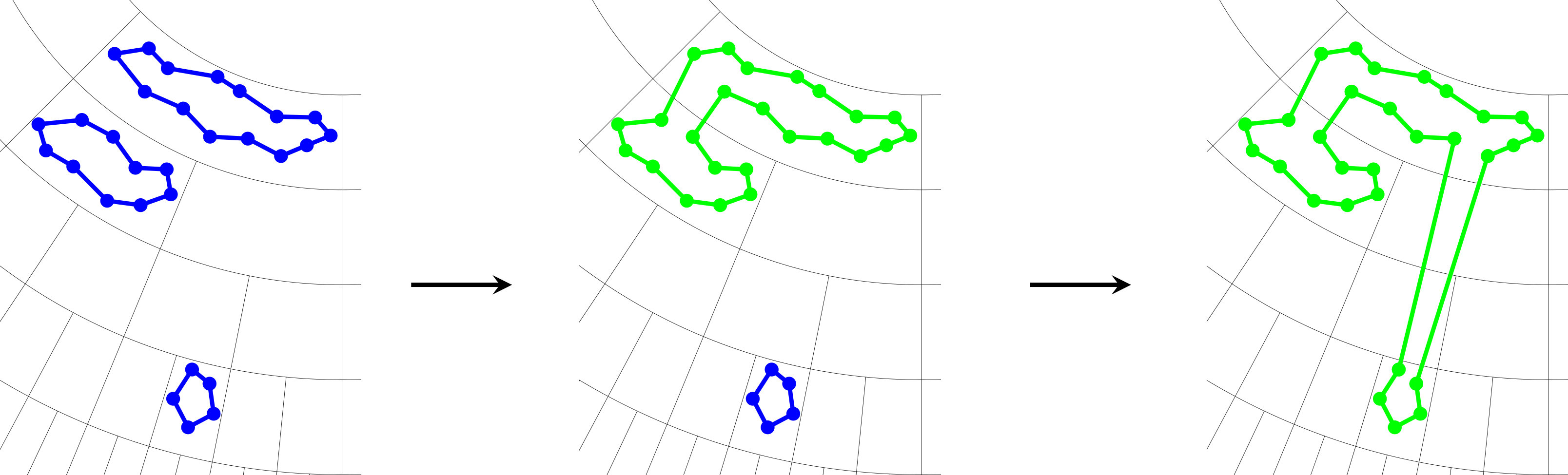 Figure 1
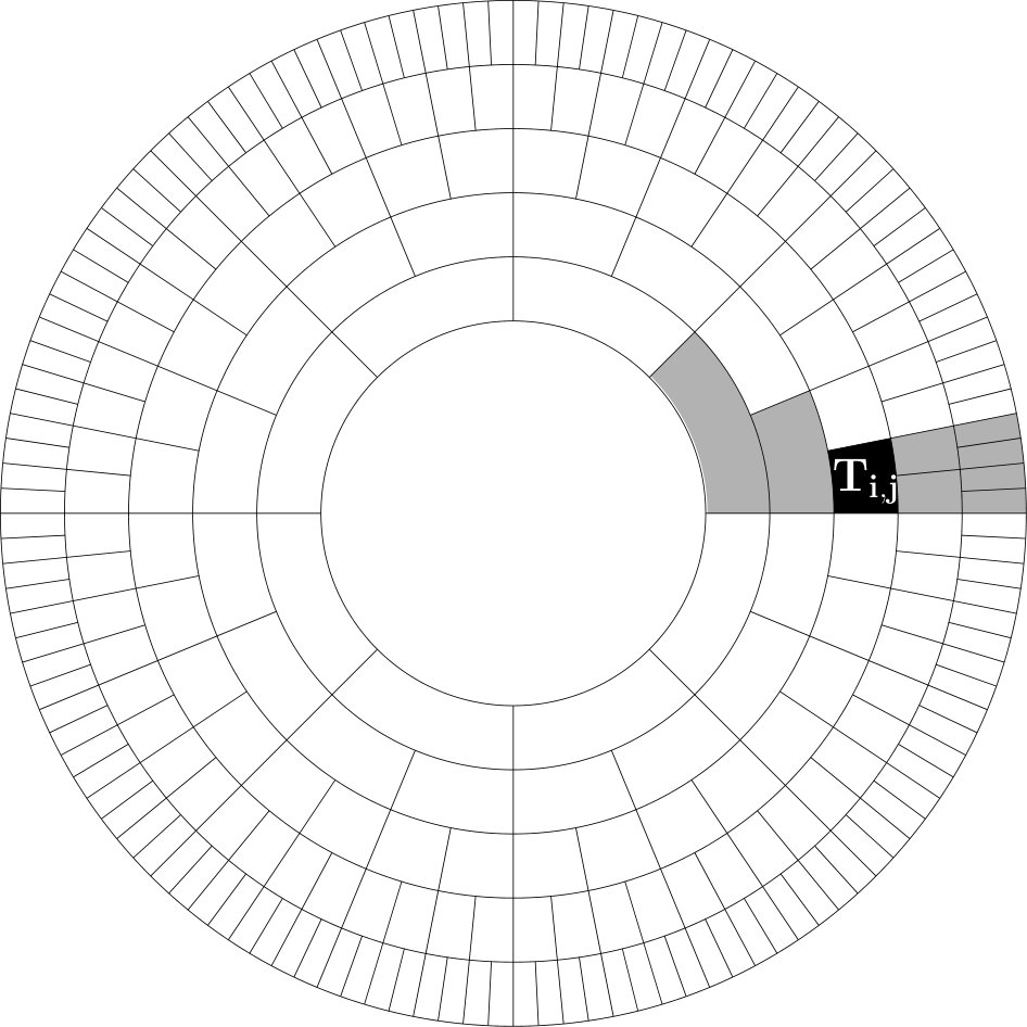 Figure 2
Peer Reviews
No public reviews on file for this paper yet. If you reviewed it on a platform where reviews are public (OpenReview, ICLR, NeurIPS, ICML), you can paste yours below so the community can read it here.
Videos
No videos yet. Explain this paper in a talk, walkthrough, or lecture? Add one.
\usetkzobj
all
Hamilton cycles and perfect matchings in the KPKVB model
Nikolaos Fountoulakis School of Mathematics, University of Birmingham, United Kingdom. E-mail: [email protected]). Research partially supported by the Alan Turing Institute, grant no. EP/N510129/1.
Dieter Mitsche Institut Camille Jordan, Université Jean Monnet, France. E-mail: [email protected].
Tobias Müller Benoulli Institute, Groningen University, The Netherlands. E-mail: [email protected]. Research partially supported by NWO grants 639.032.529 and 612.001.409.
Markus Schepers Benoulli Institute, Groningen University, The Netherlands. E-mail: [email protected]. Research partially supported by NWO grant 639.032.529
Abstract
In this paper we consider the existence of Hamilton cycles and perfect matchings in a random graph model proposed by Krioukov et al. in 2010. In this model, nodes are chosen randomly inside a disk in the hyperbolic plane and two nodes are connected if they are at most a certain hyperbolic distance from each other. It has been previously shown that this model has various properties associated with complex networks, including a power-law degree distribution, “short distances” and a non-vanishing clustering coefficient. The model is specified using three parameters: the number of nodes , which we think of as going to infinity, and , which we think of as constant. Roughly speaking controls the power law exponent of the degree sequence and the average degree.
Here we show that for every and sufficiently small, the model does not contain a perfect matching with high probability, whereas for every and sufficiently large, the model contains a Hamilton cycle with high probability.
1 Introduction
A Hamilton cycle in a graph is a cycle which contains all vertices of the graph. A graph is called Hamiltonian if it contains at least one Hamilton cycle. A matching is a set of edges that do not share endpoints and a perfect matching is a matching that covers all vertices of the graph.
Hamilton cycles and perfect matchings are classical topics in graph theory. Historically the existence of Hamilton cycles and perfect matchings in a random graph has been a central theme in the theory of random graphs as well. In particular, in the theory of the Erdős-Rényi model the threshold for having a Hamilton cycle as well as the simultaneous emergence in the random graph process of a Hamilton cycle together with having minimum degree at least two are among the classic results in the field [7, 2, 19, 26, 20]. In the context of random geometric graphs in the Euclidean plane, analogous results have been obtained [9, 4, 23]. The emergence of Hamilton cycles was also considered in other models, including the preferential attachment model [13] and the random -regular graph model [27].
In this paper, we will consider the problem of the existence of a Hamilton cycle and a perfect matching in a model of random graphs that involves points taken randomly in the hyperbolic plane. This model was introduced by Krioukov, Papadopoulos, Kitsak, Vahdat and Boguñá [21] in 2010 - we abbreviate it as the KPKVB model. We should however note that the model also goes by several other names in the literature, including hyperbolic random geometric graphs and random hyperbolic graphs. The model was intended to model complex networks and, in particular, it is motivated by the assumption that the properties of complex networks are the expression of a hidden geometry which expresses the hierarchies among classes of nodes of the network. Krioukov et al. postulate that this geometry is hyperbolic space.
The KPKVB model
Given a fixed constant and a natural number , we let , or equivalently . Also, let .
The hyperbolic plane is a surface with constant Gaussian curvature . It has several convenient representations (i.e. coordinate maps), including the Poincaré halfplane model, the Poincaré disk model and the Klein disk model. A gentle introduction to hyperbolic geometry and these representations of the hyperbolic plane can for instance be found in [28]. Throughout this paper we will be working with a representation of the hyperbolic plane using hyperbolic polar coordinates. That is, a point is represented as , where is the hyperbolic distance between and the origin and as the angle between the line segment and the positive -axis (Here, when mentioning “the origin” and the angle between the line segment and the positive -axis, we think of embedded as the the Poincaré disk in the ordinary euclidean plane.) We shall denote by the hyperbolic disk of radius around the origin , and by we denote the hyperbolic distance between two points .
The vertex set of the KPKVB random graph consists of i.i.d. points in with probability density function
[TABLE]
for and .
When the distribution of given by (1) is the uniform distribution on . For general Krioukov et al. [21] call this the quasi-uniform distribution on . In fact, for general it can be viewed as the uniform distribution on a disk of radius on the hyperbolic plane with curvature .
The KPKVB random graph is the random graph whose vertex set is a set of points of chosen i.i.d. according to the -quasi uniform distribution, where any two of them are joined by an edge if they are within hyperbolic distance at most .
Krioukov et al. [21] observed that the distribution of the degrees in follows a power law with exponent , for . This was verified rigorously by Gugelmann et al. in [15]. Note that for , this quantity is between 2 and 3, which is in line with numerous observations in networks which arise in applications (see for example [3]). In addition, Krioukov at al. observed, and Gugelmann et al. proved rigorously, that the (local) clustering coefficient of the graph stays bounded away from zero a.a.s. Here and in the rest of the paper we use the following notation: If is a sequence of events then we say that occurs asymptotically almost surely (a.a.s.), if as .
Krioukov et al. [21] observed also that the average degree of is determined via the parameter for . This was rigorously verified in [15] too. In particular, they proved that the average degree tends to in probability.
In [5], it was established that is the critical point for the emergence of a giant component in . In particular, when , the fraction of the vertices contained in the largest component is bounded away from 0 a.a.s., whereas if , the largest component is sublinear in a.a.s. For , the component structure depends on . If is large enough, then a giant component exists a.a.s., but if is small enough, then a.a.s. all components are sublinear [5].
In [11] this picture is sharpened. There, the first and the third author showed that the fraction of vertices belonging to the largest component converges in probability to a constant which depends on and . For , the existence of a critical value is established such that when crosses a giant component emerges a.a.s. [11]. In [17] and [18], the second author together with Kiwi considered the size of the second largest component and showed that when , a.a.s., the second largest component has polylogarithmic order with exponent .
Apart from the degree sequence, clustering and component sizes, the graph distances in this model have also been considered. In [17] and [12] a.a.s. polylogarithmic upper and lower bounds on the diameter of the largest component are shown, and in [24], these were sharpened to show that is the correct order of the diameter. Furthermore, in [1] it is shown that for the largest component is what is called an ultra-small world: it exhibits doubly logarithmic typical distances.
Results on the global clustering coefficient were obtained in [8], and on the evolution of graphs on more general spaces with negative curvature in [10]. The spectral gap of the Laplacian of this model was studied in [16].
The first and third author together with Bode [6], showed that is the critical value for connectivity: that is, when , then is a.a.s. connected, whereas is a.a.s. disconnected when . The second half of this statement is in fact already immediate from the results of Gugelmann et al. [14] : there it is shown that for , a.a.s., there are linearly many isolated vertices. For , the probability of connectivity tends to a limiting value that is function of that is continous and non-decreasing and that equals one if and only if .
Our results
In the present paper, we explore the existence of Hamilton cycles and perfect matchings in the model. In the light of the result on isolated vertices mentioned above, the question is non-trivial only for . A perfect matching trivially cannot exist when is odd. For this reason we find it convenient to switch to considering near perfect matchings from now on. That is, matchings that cover all but at most one vertex. (So if is even a near perfect matching is the same as a perfect matching; and the existence of a Hamilton cycle implies the existence of a near perfect matching.)
Our main results shows that in the regime regime, a.a.s., the existence of a Hamilton cycle as well as of a (near) perfect matching has a non-trivial phase transition in :
Theorem 1.1**.**
For all positive real , there are constants and such that the following hold. For all , the random graph a.a.s. does not have a near perfect matching (and consequently no Hamilton cycle either). For all , a.a.s. has a Hamilton cycle.
To our knowledge, this is the first time this problem is considered for the model. We conjecture that the dependence on is sharp.
Conjecture 1.2**.**
For every there exists a critical such that when a.a.s. has no near perfect matching, whereas if then a.a.s. has a Hamilton cycle.
A natural question to ask is what happens in the case . Does there exist large enough so that the graph a.a.s. becomes Hamiltonian in this case as well?
It would also be interesting to explore the relation of Hamiltonicity with the property of 2-connectivity. If the above conjecture is true, is there a similar behaviour for the property of 2-connectivity? If yes, are the corresponding critical constants equal?
Outline of proof. The proof of Theorem 1.1 has two parts: in a nutshell, in the first part we show that for small enough, the number of vertices close to the boundary of the disk of radius having no neighbor close to the boundary of the disk will be bigger than the total number of vertices relatively close to the centre of the disk. Hence, the former vertices would have to be all matched to distinct vertices close to the centre of the disk, but that cannot happen. For the second part, we show that for large enough, we can tessellate the disk in such a way, so that iteratively, from the boundary towards the center of the disk, we can maintain a set of vertex-disjoint cycles and isolated points, which will eventually be merged close to the centre. The fact that is large enough makes the density of vertices in each cell of the tessellation high enough so that this procedure terminates successfully.
2 Preliminaries
2.1 Probabilistic preliminaries
To prove Theorem 1.1, we will perform our analysis in the poissonisation of the model. There, the vertex set is the point set of a Poisson point process on with points on average. Although the independence that accompanies the Poisson point process facilitates our proofs, when doing standard de-poissonisation, we need to show a slightly stronger version of Theorem 1.1. We give details here.
We denote the Poissonized version of the KPKVB model by . The vertex set of this random graph is the set of points of the Poisson point process on with intensity . The set of edges of consists of those pairs of points of which are at hyperbolic distance at most . Alternatively, the Poissonized KPKVB model can be constructed as follows. Consider an infinite supply of i.i.d. points , chosen according to the -quasi uniform distribution, and a Poisson random variable . The vertex set of is now the set of points and again we add edges between pairs at hyperbolic distance at most .
The function is the intensity measure associated with . This means in particular that for any Borel subset the expected number of points that fall in equals
[TABLE]
We set ; hence . An elementary, but key, observation is that conditional on , the process is distributed as . In other words, the probability space of the process can be realised as the space of conditional on .
The following observation is well known. We include its proof here for completeness.
Lemma 2.1**.**
Let be a graph property (formally a family of graphs closed under isomorphism). We then have that
[TABLE]
Thus, if , then .
Proof.
By Stirling’s formula
[TABLE]
So as , writing :
[TABLE]
Therefore, if , we deduce that . ∎
We then apply a standard depoissonisation technique: using Lemma 2.1, we will develop our arguments in the poissonisation of the KPKVB model. More precisely, we will show that satisfies certain events with sufficiently high probability (that is, with probability at least , and we then use Lemma 2.1 to deduce that also satisfies them a.a.s., that is, with probability .
Another useful tool that will allow us to compute expectations of sums over the points of is the Campbell-Mecke formula. Let be a point process on a metric space with density . Let be the set of all countable point configurations in equipped with the -algebra of the point process (that is, for any open subset and any non-negative integer define a basic measurable subset of which consists of all configurations which have exactly points in ). Now, let be a measurable function. The Palm theory of Poisson point processes on metric spaces [22] yields:
[TABLE]
where the sum ranges over all those -tuples of points which contain no repetitions. We also use the following form of Chernoff’s bound:
Lemma 2.2**.**
For a Poisson random variable with expectation , and a positive integer ,
[TABLE]
where for ; in particular if it holds that .
A proof can for instance be found in [25].
2.2 Geometric preliminaries
For two points and in , we let be their angular distance which we define as:
[TABLE]
Note that .
The hyperbolic law of cosines relates the angular distance between two points with their hyperbolic distance:
[TABLE]
Now, for , we let be such that
[TABLE]
For two points with and , if , then . Equation (3) implies that if and only if .
The ball of radius around inside is thus defined as
[TABLE]
If is a vertex either in the vertex set of or in the vertex set of , then it is adjacent precisely to any other vertex that belongs to .
It will be convenient for our analysis to express explicitly as a function of . We will make use of the following Lemma from [11], which does this.
Lemma 2.3** ([11], Lemma 28).**
There exists a constant such that for every and sufficiently large, the following holds: for every with , we have
[TABLE]
Moreover, if , then .
3 Non-existence of perfect matching for sufficiently small
The following theorem yields the first part of Theorem 1.1.
Theorem 3.1**.**
For all positive real , there is a such that for all , the random graph does not have a near perfect matching w.p. .
Proof.
The strategy is as follows. Let . Let be number of vertices with radial coordinate at least and with no neighbour with radial coordinate at least . Let be the number of vertices with radial coordinate at most . Hence, is the number of points of inside the disk of radius and is a subset of the annulus of width . If there is a perfect matching, then because a vertex with no neighbour with radius at least must be matched to a vertex with radius less than , so distinct vertices counted by must be matched to distinct vertices counted by . If it is shown that and are concentrated around their expectation w.p. and that and as and , then there will be no near perfect matching and hence no Hamilton cycle w.p. .
We observe that , where
[TABLE]
As is Poisson distributed, we deduce that . (Here and elsewhere we write to denote that .) By Chebyshev’s inequality, it follows that for all
[TABLE]
Our aim now is to give a lower bound on . To this end, we will show that .
For a point we let denote the indicator random variable which is equal to 1 if and only if . In other words, is equal to 1 if and only if no point of is contained in .
We can write
[TABLE]
The Campbell-Mecke formula (2) will allow us to calculate the expected value of :
[TABLE]
where the first equality holds since , if and only if and the last one since is invariant with respect to .
We have
[TABLE]
and, therefore,
[TABLE]
We can give an asymptotic approximation to this integrand. From Lemma 2.3, we infer that for large enough, uniformly over all :
[TABLE]
and
[TABLE]
Therefore,
[TABLE]
But . We use that , and set
[TABLE]
Thus, for sufficiently enough . So for any such
[TABLE]
If we substitute this into (3), we get the following lower bound:
[TABLE]
As , we have that . Select sufficiently small so that
[TABLE]
Thereafter, we choose sufficiently small so that
[TABLE]
We will use Chebyshev’s inequality to show that w.p.
[TABLE]
Since w.p. , the union bound implies w.p. .
We will show that . To bound the variance, let us set
[TABLE]
We write
[TABLE]
We will use the Campbell-Mecke formula (2) to calculate these sums. For the former one, we have:
[TABLE]
Let . We claim that for sufficiently large, , if . Indeed, Lemma 2.3 implies that for any , we have , for sufficiently large. Thus, for any such , if , then . This would imply that . So if , then .
This implies that for sufficiently large, whenever , we have . Moreover, . So,
[TABLE]
Regarding the second term, we use that and bound
[TABLE]
These two imply that
[TABLE]
Chebyshev’s inequality yields
[TABLE]
∎
4 Existence of Hamilton cycles for sufficiently large
The aim of this section is to prove the existence of a Hamilton cycle in when is large enough with sufficiently high probability.
Theorem 4.1**.**
For all positive real , there is a such that for all , the random graph has a Hamilton cycle and hence also a near perfect matching with probability .
4.1 A useful tiling
We consider the following tiling
[TABLE]
where , for , and , . We call admissible if they satisfy these constraints. Note that for all admissible , the parameter is an integer and, in fact, a power of , as the exponent is an integer. Moreover, for the exponent is also at least .
We call the collection of tiles with a fixed given the -th layer. These are the tiles in the -th annulus where we start counting from zero at the boundary of the disk. Note that there are tiles in the -th layer and the tiling covers the annulus with exterior radius and interior radius (in particular, the most interior layer is contained in the smaller disk with radius around the origin). A schematic picture is shown in Figure 1.
We say that a tile is below the tile , if and the sector defined by contains .
Lemma 4.2** (Adjacency among the tiles).**
For admissible indices , any point is within distance from any point in any tile below the tile .
Proof.
Let and be a vertex in any tile below tile (in the sense of the statement above). Note that must hold. Then, the angular distance between and is at most the angular width of the tile which is
[TABLE]
On the other hand, we know that the radial coordinates satisfy and . If , we have adjacency by the triangle inequality. If and using that (as remarked earlier), we distinguish two cases:
If (with as in Lemma 2.3), then by the last part of Lemma 2.3, it holds that
[TABLE] 2. 2.
Otherwise we may assume that holds, while still . Therefore, , hence the error term in Lemma 2.3 is and it follows that
[TABLE]
We conclude that from which the claim follows. ∎
We will denote by the number of points falling into .
Lemma 4.3** (Expected number of points in a tile).**
Let . For admissible indices , the expected number of points falling into satisfies:
[TABLE]
Proof.
The expected number of points falling into is given by:
[TABLE]
As , we have that , and hence
[TABLE]
[TABLE]
and
[TABLE]
Furthermore, . We conclude:
[TABLE]
Finally, using that , that is, , yields the claim. ∎
4.2 A procedure for finding a Hamilton cycle
In this subsection we describe the strategy of our procedure for finding a Hamilton cycle in a graph which is embedded in the hyperbolic disk and which makes use of the tiling defined above. Roughly speaking, the procedure iterates through the layers of the tiling, working upwards from the [math]-th layer to layer , gathering a suitable collection of vertex-disjoint cycles and isolated vertices. When processing the tile , it merges as many vertex-disjoint cycles and isolated points from previous iterations that are below the tile as possible. Once the procedure has reached the maximum layer which is completely contained in the smaller disk with radius , the procedure attempts to merge all the remaining cycles and points.
We now describe the procedure in more detail. For each tile we will define a random variable called demand, which will be used later in the probabilistic analysis to show that the procedure terminates successfully. Recall that denotes the number of points in tile and note that the collection of for admissible are independent Poisson random variables for the poissonised KPKVB model.
Lemma 4.4** (Cycle merging, see Figure 2).**
If the vertices strictly below tile can be covered by vertex-disjoint cycles and isolated vertices and the number of vertices in tile , , then the set of all vertices below (including those in ) can be covered by cycles and points.
Furthermore, if additionally , then the vertices below can be covered by a single cycle which has edges within .
Proof.
If , then the vertices in form a cycle by Lemma 4.2. Each of its edges can be used to merge this cycle in with a cycle or point strictly below : to pick up a cycle, use an edge of the cycle in and choose any edge from the cycle to be picked up. By Lemma 4.2, the four endpoints form a clique and therefore, we can go along the edges , then the cycle to be picked up (without the edge ), and finally along to bring us back to the cycle in . To pick up a vertex below, we can just use the edges and instead of .
If , then all edges of the original cycle in will be used and we end up with cycles and points below (and including) . If , then all cycles and points strictly below become part of the original cycle in and edges of the cycle in remain unused and part of the final cycle. ∎
The demand random variables for admissible are defined in terms of the point counts as follows. For and we set:
[TABLE]
and, for and we set:
[TABLE]
In particular and are independent for , since they depend on disjoint regions. Also, the are i.i.d. random variables with values in satisfying
[TABLE]
where we used the notation .
Lemma 4.5**.**
For admissible indices , if , then the vertices below (and in) can be covered by at most vertex-disjoint cycles and isolated points (in total).
Moreover, if and , then the vertices below (and in) can be covered by exactly one cycle which has at least one edge which is completely contained in .
Proof.
The proof is by induction on . For , the claim is clear because then implies that there is either one cycle or no vertex in .
For , assuming the claim for we show it for . By the induction hypothesis, the vertices below (, respectively) can be covered by (, respectively) many vertex-disjoint cycles and isolated points. Thus, the vertices strictly below can be covered by many vertex-disjoint cycles and isolated points in total. If , then by Lemma 4.4, the vertices below can be covered by
[TABLE]
If , then the points in just remain as single points and the area in and below can be covered by at most vertex-disjoint cycles and isolated points.
In particular, if , the points in the area in and below can be covered by one cycle or point. If , then the condition and the definition of imply that there are at least 3 points in . Hence, the vertices in and below can be covered by exactly one cycle, which will have at least one edge with both endpoints inside (using that ). ∎
Lemma 4.6**.**
If for and for all , then there is a Hamilton cycle.
Proof.
Firstly, we observe that for , if , then all vertices in and below can be covered by one cycle that contains an edge whose endpoints are both in by Lemma 4.5. Taking such an edge for and , the four endpoints form a clique by the triangle inequality because all radial coordinates are at most and hence the cycle of can be taken as a detour to the cycle of as in the proof of Lemma 4.4. As a result, we have a cycle covering all vertices below and and with an edge inside the -th layer. We can repeat this procedure to merge this resulting cycle also with those in . We will end up with one cycle covering all vertices below all tiles , and this cycle contains an edge whose endpoints are both in the inner disk with radius . The remaining vertices in the inner disk, that are not in any tile, form a clique and in particular can be covered by a cycle. We can again merge this cycle with the one we created earlier via the same trick. ∎
4.3 Probabilistic lemmas which ensure the a.a.s. successful termination of the procedure
In this subsection we show that the algorithm explained previously works successfully for the poissonised KPKVB model with many vertices (the standard depoissonisation of Lemma 2.1 gives then the result in the standard KPKVB model). Lemma 4.8 of this section shows the exponential decay of the demand random variables, which we then use in Lemma 4.9 to show that the demand random variables are simultaneously zero in the maximum layer. Appealing to Lemma 4.6, we can then conclude that this makes the algorithm work.
4.3.1 Sub-exponential tail decay of demand
We first show the following technical lemma:
Lemma 4.7**.**
For all real , there exists such that for all , for all we have: .
Proof.
Pick such that ; this is possible as . We prove the lemma in the following way: in the first step we verify that for we have , and then we show that the left-hand side of the inequality is monotone decreasing in (by showing that its derivative with respect to is negative). Since the right-hand side is independent of , this clearly implies the lemma.
For the first step, we need to show that . Using that , and , we note that the left-hand side of the inequality can be bounded from above by
[TABLE]
Now, if we plug in , this upper bound is at most by the choice of . The derivative in of the latter expression is
[TABLE]
which is negative for for all , Therefore, the upper bound is monotone decreasing in and hence, for all and , we have , concluding the first step.
For the second step, we need to verify that the derivative of is negative in : using the assumptions of and , we have
[TABLE]
The lemma follows. ∎
We are now ready to state and prove the main lemma of this section.
Lemma 4.8**.**
There is a constant such that for and sufficiently large, for all admissible , and all :
[TABLE]
Proof.
Set , and , for . So, in particular, we have .
We prove the lemma by induction on . For the base case , the claim is clear for because , so . For ,
[TABLE]
where the equality follows by Lemma 4.3. In particular, by choosing large enough, it holds that for .
For the inductive step, assume the statement is true for with .Note that as and are independent, we can apply the induction hypothesis to and to get
[TABLE]
Define
[TABLE]
let as in Lemma 4.7 and set
[TABLE]
We make a case distinction in .
Case 1: .
Using the definition of and by (4.3.1), we have
[TABLE]
Now, we can apply Lemma 4.7 to to deduce that
[TABLE]
We infer that
[TABLE]
where the third line follows by choice of and the definition of the sequence , which implies that .
Case 2: .
Let . We first observe that for all :
[TABLE]
and
[TABLE]
To see that this holds, note that as (see Lemma 4.3), we can take any and then pick such that for all and all , the claims hold (as the right-hand side is independent of and grows at most polynomially in whereas grows exponentially in ). Then, as the right-hand sides of (6) and (7) are independent of , we can pick large enough such that (6) and (7) also hold for .
Thus, (6) and (7) hold for all and all .
We have
[TABLE]
We split the sum into two parts: for , we apply Lemma 2.2 with and and hence, . Therefore, and we get
[TABLE]
By (missing) 6, it follows that
[TABLE]
So, we have for the first part of the sum
[TABLE]
For the second part, we have . By (missing) 7, . By (4.3.1) and Lemma 4.7 with it holds that
[TABLE]
With this, we can also bound from above the second sum:
[TABLE]
where the last inequality follows from the choice of and the fact that .
By combining both sums, we conclude that also for as in Case 2, , and the lemma follows. ∎
4.3.2 Deriving Theorem 4.1
Finally, Theorem 4.1 is a result of the following lemma together with Lemma 4.6.
Lemma 4.9**.**
Let , sufficiently large. Then
[TABLE]
Proof.
First, let us recall that the number of tiles in the th layer is . For , it follows that . Furthermore, .
We have
[TABLE]
By the union bound over all tiles in layer
[TABLE]
Now we observe that if and and all hold, then since . Hence if all three of these conditions hold then . In other words, if then or or .
Therefore,
[TABLE]
For the first two terms, we use Lemma 4.8, taking sufficiently large, and for the third term, we apply Lemma 2.2. We get
[TABLE]
Using that , it follows that . Since , we obtain
[TABLE]
and the lemma follows. ∎
The reference list from the paper itself. Each links out to its DOI / PubMed record.
- 1[1] M.A. Abdullah, M. Bode, and N. Fountoulakis. Typical distances in a geometric model for complex networks. Internet Mathematics , 1, 2017.
- 2[2] M. Ajtai, J. Komlós, and E. Szemerédi. First occurrence of Hamilton cycles in random graphs. North-Holland Mathematics Studies , 115:173–175, 1985.
- 3[3] R. Albert and A.-L. Barabási. Statistical mechanics of complex networks. Rev. Mod. Phys. , 74(1):47–97, 2002.
- 4[4] J. Balogh, B. Bollobás, M. Krivelevich, T. Müller, and M. Walters. Hamilton cycles in random geometric graphs. The Annals of Applied Probability , 21(3):1053–1072, 2011.
- 5[5] M. Bode, N. Fountoulakis, and T. Müller. On the largest component of a hyperbolic model of complex networks. Electronic Journal of Combinatorics , 22(3), 2015. Paper P 3.24, 43 pages.
- 6[6] M. Bode, N. Fountoulakis, and T. Müller. The probability that the hyperbolic random graph is connected. Random Structures Algorithms , 49(1):65–94, 2016.
- 7[7] B. Bollobás. The evolution of sparse graphs. In Graph Theory and Combinatorics , pages 35–57, London, 1984. Academic Press.
- 8[8] E. Candellero and N. Fountoulakis. Clustering and the hyperbolic geometry of complex networks. Internet Mathematics , 12:2–53, 2016.