Minimizing lattice structures for Morse potential energy in two and three dimensions
Laurent B\'etermin (QMATH, University of Copenhagen)

TL;DR
This paper analyzes the optimal lattice structures for Morse potential energy in two and three dimensions, identifying conditions for minimality and proposing a conjecture on the global minimizer with implications for material modeling.
Contribution
It provides a rigorous proof of the triangular lattice's optimality in 2D, numerical studies of 3D lattice optimality, and a conjecture on the transition of minimal structures as parameters vary.
Findings
Triangular lattice is proven optimal in 2D within certain densities.
Numerical evidence supports local optimality of cubic, FCC, and BCC lattices in 3D.
A conjecture suggests a transition from BCC/FCC to HCP as the Morse potential parameter increases.
Abstract
We investigate the local and global optimality of the triangular, square, simple cubic, face-centred-cubic (FCC), body-centred-cubic (BCC) lattices and the hexagonal-close-packing (HCP) structure for a potential energy per point generated by a Morse potential with parameters . The optimality of the triangular lattice is proved in dimension 2 in an interval of densities. Furthermore, a complete numerical investigation is performed for the minimization of the energy with respect to the density. In dimension 3, the local optimality of the simple cubic, FCC and BCC lattices is numerically studied. We also show that the square, triangular, cubic, FCC and BCC lattices are the only Bravais lattices in dimensions 2 and 3 being critical points of a large class of lattice energies (including the one studied in this paper) in some open intervals of densities, as we observe for the…
Click any figure to enlarge with its caption.
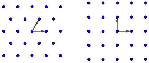 Figure 1
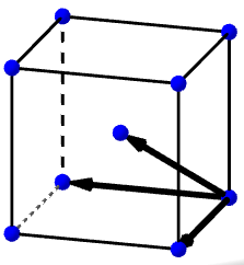 Figure 2
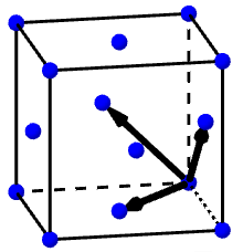 Figure 3
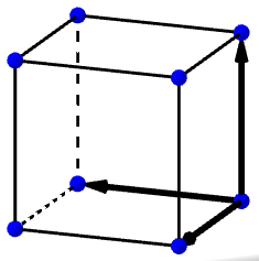 Figure 4
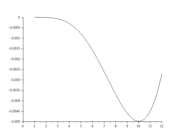 Figure 5
 Figure 6
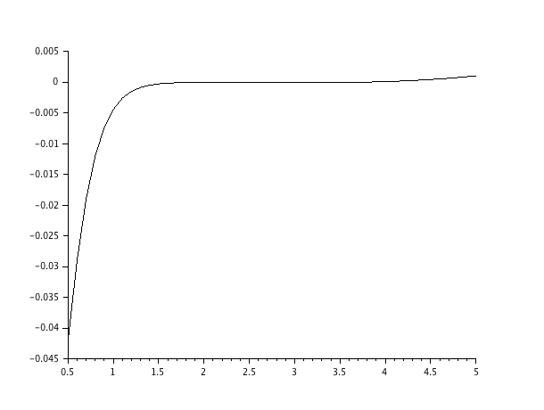 Figure 7
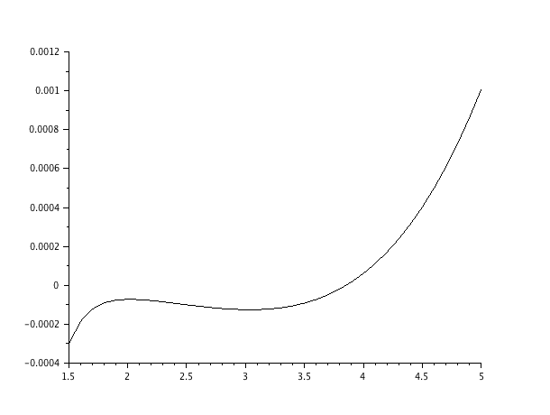 Figure 8
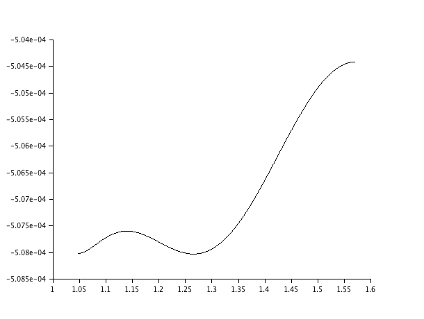 Figure 9
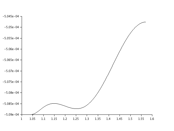 Figure 10
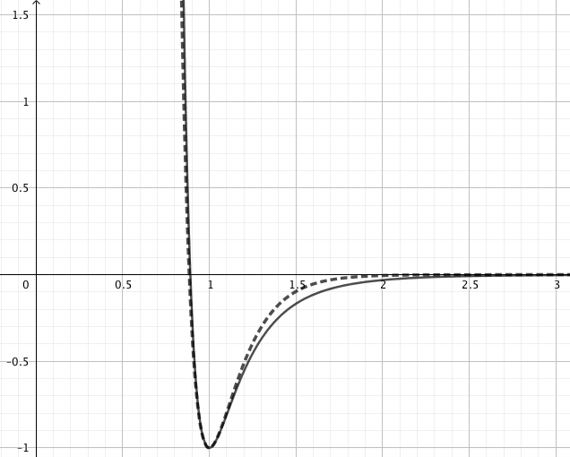 Figure 11
 Figure 12
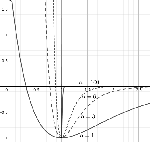 Figure 13
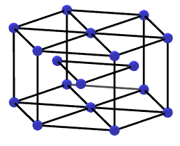 Figure 14
| Area | Minimizer in |
|---|---|
| (M): | Triangular |
| (LJ): | |
| (M): | Rhombic |
| (LJ): | |
| (M): | Square |
| (LJ): | |
| (M): | Rectangular |
| (LJ): | (more and more thin as ) |
| Values of such that is minimal for | Condition(s) satisfied | |
|---|---|---|
| 1 | ||
| 2 | ||
| 3 | ||
| 4 | ||
| 5 | ||
| 6 | ||
| 7 | ||
| 8 | ||
| 9 | , | |
| 10 | , |
| Lattice | (M) | (LJ) | (M) | (LJ) |
|---|---|---|---|---|
| Local minimum | ||||
| Local maximum | ||||
| Saddle point |
| Lattice | |||
|---|---|---|---|
| Local min | (M): | (M): | (M): |
| (LJ): | (LJ): | (LJ): | |
| Local max | (M): | (M): | (M): |
| (LJ): | (LJ): | (LJ): | |
| Saddle point | (M): | (M): | (M): |
| (LJ): | (LJ): | (LJ): |
Peer Reviews
No public reviews on file for this paper yet. If you reviewed it on a platform where reviews are public (OpenReview, ICLR, NeurIPS, ICML), you can paste yours below so the community can read it here.
Videos
No videos yet. Explain this paper in a talk, walkthrough, or lecture? Add one.
Minimizing lattice structures for Morse potential energy
in two and three dimensions
Laurent Bétermin
QMATH, Department of Mathematical Sciences, University of Copenhagen,
Universitetsparken 5, DK-2100 Copenhagen Ø, Denmark.
[email protected]. ORCID id: 0000-0003-4070-3344
(date)
Abstract
We investigate the local and global optimality of the triangular, square, simple cubic, face-centred-cubic (FCC), body-centred-cubic (BCC) lattices and the hexagonal-close-packing (HCP) structure for a potential energy per point generated by a Morse potential with parameters . In dimension 2 and for large enough, the optimality of the triangular lattice is shown at fixed densities belonging to an explicit interval, using a method based on lattice theta function properties. Furthermore, this energy per point is numerically studied among all two-dimensional Bravais lattices with respect to their density. The behaviour of the minimizer, when the density varies, matches with the one that has been already observed for the Lennard-Jones potential, confirming a conjecture we have previously stated for differences of completely monotone functions. Furthermore, in dimension 3, the local minimality of the cubic, FCC and BCC lattices are checked, showing several interesting similarities with the Lennard-Jones potential case. We also show that the square, triangular, cubic, FCC and BCC lattices are the only Bravais lattices in dimensions 2 and 3 being critical points of a large class of lattice energies (including the one studied in this paper) in some open intervals of densities, as we observe for the Lennard-Jones and the Morse potential lattice energies. More surprisingly, in the Morse potential case, we numerically found a transition of the global minimizer from BCC, FCC to HCP, as increases, that we partially and heuristically explain from the lattice theta functions properties. Thus, it allows us to state a conjecture about the global minimizer of the Morse lattice energy with respect to the value of . Finally, we compare the values of found experimentally for metals and rare-gas crystals with the expected lattice ground-state structure given by our numerical investigation/conjecture. Only in a few cases does the known ground-state crystal structure match the minimizer we find for the expected value of . Our conclusion is that the pairwise interaction model with Morse potential and fixed is not adapted to describe metals and rare-gas crystals if we want to take into consideration that the lattice structure we find in nature is the ground-state of the associated potential energy.
AMS Classification: Primary 74G65 ; Secondary 82B20, 35Q40.
Keywords: Morse potential; Lattice energy; Ground-state; Crystallization; Energy minimization; Stability.
Contents
-
2 Optimality of the triangular lattice in : rigorous results
-
3 A general result about volume-stationary lattices - Proof of Theorems 1.5 and 1.7
-
5.3 Heuristic arguments supporting Conjecture 1.8 based on duality relation
-
5.4 Comparison of our conjecture with some experimental values of and
1 Introduction and main results
A fundamental question in Mathematical Physics that has been actively investigated recently is the following “Crystal Problem” (also called “The crystallization conjecture” see e.g. [55, 18]): Why are solids crystalline? Answering this question in a rigorous mathematical way is known to be extremely challenging, even though the interactions between atoms or molecules are assumed to be a sum of pairwise potentials. Whereas the one-dimensional version of this problem is well-understood [65, 66, 67, 35, 14], only few results have been proved in dimensions and for models consisting of short-range interactions [38, 44, 45, 43, 34], perturbations of the hard-sphere potential [63, 30, 33] and oscillating functions [61].
In 1929, Morse [50] solved the three-dimensional Schrödinger equation with potential
[TABLE]
known now as the “Morse Potential”, where is the euclidean norm in . This is an attractive-repulsive potential (see Figure 1 for a plot), i.e. a decreasing-increasing potential having one well. Parameters and respectively represent the minimizer of and the hardness of the interaction (as increases, goes to a hard-core potential, see Figure 1). This potential is known to be a canonical model for social aggregation – e.g. swarming and flocking – as explained in [7, Sect. 4] (see also [29, 21] and references therein). Furthermore, it has been shown (see e.g. [39]) that provides a description of the vibrational properties of rare-gas crystals which is better than the one given by the quantum harmonic oscillator (see also [56, 2, 54, 6]). Moreover, interactions in cubic metals are also well-described by the Morse potential, as explained in [36, 42, 60, 47, 53, 40] and [41, p. 22]. The values of parameters can then be computed from experimental data for many metals and rare-gas crystals.
Crystallization problems for Morse potential have not received so much attention. Ventevogel and Nijboer [66, p. 276] pointed out the fact that, even in dimension 1, any general crystallization result is difficult to reach for (they claim to have the solution among one-dimensional periodic configurations with 2 and 3 points in each period). However, in a recent paper, Bandegi and Shirokoff [5, Sect. 6.1] give numerical evidences for the global optimality of the equidistant configuration for some values of the density and the parameters of the Morse potential, using convex relaxation arguments. In higher dimension, no such result exists and only local stability properties has been proved in [46], using Born’s stability criteria for crystals, following the methods developed in [19, 48].
Instead of investigating the pure Crystal Problem involving – i.e. minimizing the interaction energy among all the possible point configurations – we choose to study the minimization of the energy per point among periodic lattices where the points are interacting via a Morse potential. This point of view has been taken in several previous works in Number Theory [57, 31, 32, 22, 28, 49, 59, 25, 26, 37], optimal point configurations problems [24] and Mathematical Physics [52, 1, 23, 58, 15, 13]. It is a natural first step for keeping or rejecting periodic structures which could be good candidates for the Crystal Problem associated to the interaction potential. We have already studied the Lennard-Jones type potential case in [17, 8, 9, 10, 16] and our goal is to give the same kind of quantitative results for the Morse potential.
Let us first define our spaces of periodic lattices. Let be the space of Bravais lattices, i.e. having the form where is a basis of , of area (in dimension , and we will note it ) or volume (i.e. the volume of their unit cell) and be the space of all -dimensional Bravais lattices. We also write the space of all -dimensional periodic configurations, i.e. all the possible finite unions of Bravais lattices. We hence have, for any volume , . Furthermore, in dimension and , as explained for instance in [62], any Bravais lattice can be parametrized by a vector or where (resp. ) belongs to a fundamental domain containing only one copy of each lattice (it is basucally due to the reduction of quadratic forms). This parametrization will be used in Sections 4 and 5. In particular, for any of class , the gradient and the Hessian of at will be respectively denoted by and . For more details, see [10, 9]. Furthermore, the same differentation with respect to the structure can be done for periodic configurations (see e.g. [26] for details).
We now define the energy we want to focus on. Writing
[TABLE]
the goal of this paper is to investigate rigorously and numerically the energy per point defined by
[TABLE]
among Bravais lattices (or among periodic configurations). This energy, as it is the case for Lennard-Jones type potentials and for the difference of Yukawa potentials (see [8, Sec. 5]), can be seen as a difference of competitive interactions with completely monotone potentials (i.e. the functions are positive and the signs of their derivatives alternate). It has been shown in [8, Sec. 3.1] that is minimized by the triangular lattice and the square lattice is a saddle point of the energy, in for all fixed and for all , following the lattice theta function properties proved in [49]. Thus, studying the minimization on for a difference of such lattice energies must show, as in the Lennard-Jones case, many other minimizing lattices with respect to , at least in dimension 2 (see [10]).
Using a method we have developed in [17, 8], we find an interval of areas such that the triangular lattice (see Figure 2) defined by
[TABLE]
is the unique minimizer, up to rotation, of in , when is not too small. Furthermore, the non-optimality of the triangular lattice at low density (i.e. large area) can be shown as a direct consequence of [16, Thm 1.5], which is itself a consequence of Montgomery Theorem [49, Thm 1] and the functional equation for the lattice theta function [49, Eq. (2)] defined by
[TABLE]
More precisely, we prove the following result.
Theorem 1.1** (Sufficient conditions for the optimality of ).**
Let . If satisfies one of the following conditions:
- (C1)
* and ,* 2. (C2)
* and ,*
then the triangular lattice is the unique minimizer of in , up to rotation.
Furthermore, for any there exists such that for any , is not a minimizer of in .
Remark 1.2**.**
If and , then , is satisfied and, solving numerically , we find that which is then an interval of area where the triangular lattice is the minimizer of in . Other numerical values are given in Table 2.
In particular, we notice that this method does not apply for (approximatively), where none of the conditions are satisfied. This is due to the lower bound (2.3) we have used in the proof. Numerical investigations show that area bounds exist for smaller value of , but we have chosen conditions and because they are simple and tractable and we are mostly interested in the , case which is comparable to the classical Lennard-Jones potential case (1.4) (see Figure 5). Furthermore, in most of the case (for instance in [36, 42, 60, 53, 40, 56, 2, 54, 6]), the values of (rescaled such that ) computed from experimental data are larger than .
Since both conditions and are satisfied for large values of , we then derive the following consequence of Theorem 1.1 that gives an explicit interval of areas where the triangular lattice is minimal.
Corollary 1.3** (Interval of areas for the optimality of the triangular lattice when is large).**
Let where is the unique solution of on . If and satisfies
[TABLE]
*then is the unique minimizer of , up to rotation, in .
Remark 1.4**.**
We notice that, by assumption, , and therefore the optimality of the triangular lattice at very high density is not proved. We also remark that it is possible to reach any small value of by increasing (or ) and such that is minimal in for .
This result ensures the possibility to get a triangular lattice as a ground-state at a certain density (and in the neighborhood of it), using a Morse potential. However, it also shows the limits of our methods, as discussed in Section 2.3. In particular, we cannot get the optimality of the triangular lattice in the high density limit as it was the case for the Lennard-Jones type potentials in [8], and as we have numerically checked it for . A modification of the Morse potential is then proposed in Section 2.3 in order to fill this gap. Furthermore, we also remark that the whole method developed in [8] cannot be applied for the Morse potential in order to show the global optimality, in , of a triangular lattice for . Indeed, it is straightforward to prove that any global minimizer of on has an area smaller than , and it is not possible – using our method – to show that is the unique minimizer of for any , whatever and are.
We have performed a numerical investigation of the minimizers of in when varies, as it was done for the classical Lennard-Jones potential
[TABLE]
in [10]. Contrary to the latter, the lack of homogeneity of makes the systematic analysis of the local extrema of very difficult, and we cannot find explicit analytic bounds for the local optimality of and the square lattice depicted in Figure 2. We only propose, in Lemma 2.12, an asymptotic result for the local minimality of for small values of . The details of our numerical study can be seen in Section 4, based in particular on the minimization among rectangular lattices (i.e. its unit cell is a rectangle with sides of length ) and rhombic lattices (i.e. its unit cell is a rhombus with smallest angle ) where are respectively defined by
[TABLE]
The two most important observations are the following:
Global minimizer: for all , the global minimizer of in seems to be a triangular lattice, as it seems to be the case for Lennard-Jones type potentials (see [8, 10, 16]). 2. 2.
Confirmation of our conjecture: the minimizer’s transition with respect to follows the same law as the one we have observed for the classical Lennard-Jones potential in [10] This supports a conjecture we have stated in [10, Sec. 5.4] and where the same phenomenon is expected for all difference of completely monotone functions having only one well. More precisely, as increases, the evolution of the minimizer of in is depicted in Table 1, where the case has been chosen, and compared to the classical Lennard-Jones case (in such a way that and both have their absolute minimum for ). We observe a transition triangular-rhombic-square-rectangular for the minimizer of in , as increases, which seems to stay true for other values of (like for instance). As , the minimizer is rectangular and becomes more and more thin. More details are given in Section 4.2. This minimizer’s behaviour is also similar to the one appearing in the two-components Bose-Einstein Condensates described by Ho and Mueller in [51, Fig. 1 and 2]. The same phenomenon is also naturally expected in other physical and biological models involving infinite lattices and competitive interactions.
In particular, we notice that the triangular and square lattices are the only one staying critical points of in for in some open intervals. We call these lattices ‘volume-stationary’ and we have also remarked this phenomenon in [10] for the classical Lennard-Jones potential. The next result, based on Gruber’s result [37, Cor 2], shows that this property has a certain universality.
Theorem 1.5** (Volume-stationary lattices in dimension ).**
Let and be a nonzero function such that
as , we have for some , 2. 2.
for any , it holds for some Borel measure on .
For any , we define
[TABLE]
and let . There exists an open interval such that for all if and only if , thus .
Remark 1.6**.**
The same result is stated in dimension in Theorem 1.7, and a more general result (see Theorem 3.2) will be proved for -dimensional lattice energies in Section 3: all the layers of such lattices are strongly eutactic in the sense of Definition 3.1. Note that the Morse potential satisfies the assumption of the theorem because is defined by (2.1) (as well as any Lennard-Jones type potential), thus the result is actually true for (and also for the Lennard-Jones energy studied in [10]).
In dimension 3, the problem is obviously more difficult. The space of Bravais lattices with fixed volume is a five-dimensional space and only local optimality results have been proved for usual interaction potentials [32, 15, 9], even for the completely monotone potentials (see e.g. [11] for a review in the soft lattice theta function case). The only global minimality results is proved by Sarnak and Strömbergsson in [59] for the height of the three-dimensional torus (i.e. the derivative of the Epstein zeta function at the origin), using a computer assisted proof. The exact formula for the partial derivatives of are known (see e.g. [9]), but their systematic analysis is again very difficult, by lack of homogeneity of which contains exponential terms. The four important (for us, in this context) three-dimensional lattices of unit density are the simple cubic lattice , Face-Centred-Cubic (FCC) lattice , Body-Centred Cubic (BCC) lattice and the Hexagonal-Close-Packing (HCP) structure depicted in Figure 3, and defined by
[TABLE]
Using the formula proved in [9], we have numerically studied the local optimality of the cubic lattices , and for in , when varies. The results, presented in Table 4, are similar with the one found for the classical Lennard-Jones potential in [9]. In particular, we also observe that these cubic lattices are the only one staying critical points for in some open intervals of volumes . It turns out that this phenomenon, as the one observed in dimension for and and proved in Theorem 1.5, is also universal as shown in the next result, again based on Gruber’s result [37, Cor 2], and generalized in Section 3.
Theorem 1.7** (Volume-stationary lattices in dimension ).**
Let and be defined as in Theorem 1.5 with . A Bravais lattice satisfies for all where is an open interval if and only if , thus .
According to [3], it is important to notice that the global minimum for the three-dimensional Morse lattice energy in should be an HCP structure, for large parameter , which does not belong to the class of Bravais lattice we are interested in. This also holds for the Lennard-Jones potential for large exponents (see e.g. [3, 16]). Even though , using formula (1.10) we have computed the numerical values of .
Surprisingly, we numerically found the following transition of minimizers. Defining
[TABLE]
we obtain:
If , where , then ; 2. 2.
if , where , then ; 3. 3.
if , then .
It turns out that the multiple stable structures for Morse potential, Modified Morse potential and Lennard-Jones potential have been numerically studied in [3, Fig. 5]. Then, we propose the following new conjecture for the Morse potential lattice energy that will be heuristically justified (for the BCC/FCC transition) in Section 5.3, based on Sarnak-Strömbergsson conjecture [59, Eq. (43)] for the lattice theta functions defined by (1.3).
Conjecture 1.8** (Global minimizer of Morse potential lattice energy).**
Let , then there exists , such that
If , then the global minimizer of in is a BCC lattice. 2. 2.
If , then the global minimizer of in (resp. in ) is a FCC lattice (resp. a HCP structure). 3. 3.
If , then the unique minimizer of in is a FCC lattice.
This conjecture appears to be obviously more difficult to prove than the Sarnak-Strömbergsson conjectures for lattice theta functions and Epstein zeta functions described in [59, Eq. (43)-(44)], in particular for the minimization problem on .
We have compared this conjecture to the values of found from experimental quantities for metals in [36, 42, 60, 53, 40]. We observe that the real ground-states of metals match with the expected ground-state given by our conjecture, according to the experimental values of , only in few cases for both FCC and BCC structures. Details are given in Section 5.4, but it clearly appears that the pure central-force model with two-body Morse potential is not sufficiently accurate to describe metals if we want to take into consideration that their FCC or BCC structure are not only local minimizers, but global minimizers. The same holds for rare-gas crystals when we compare the expected ground-state structure with the values of the parameters found in [56, 2, 54, 6].
Another interesting fact is the similarity of the two and three-dimensional cases, respectively in the square/cubic cases and the triangular/FCC cases. This justifies the relevance of studying one (two-dimensional) layer instead of the whole crystal, even though the dimension reduction techniques described in [15] and following from the multiplicative property of the exponential function cannot be applied here. That was also observed in the Lennard-Jones case in [10, 9] and we expect this property to be true for many other repulsive-attractive potentials. It is by itself a good motivation to study two-dimensional lattice energies.
Plan of the paper. We start in Section 2 by showing Theorem 1.1 and Corollary 1.3, then explaining what are the limits of our method based on Montgomery result and finally proving the local optimality of the triangular lattice at high density. We then prove a generalization of Theorem 1.5 and Theorem 1.7 in Section 3 about Bravais lattices being critical points of energies of type in , for all in an open interval. The numerical investigation of the minimizers of is explained in Section 4, where the local optimality of the triangular and square lattices is studied and our Conjecture for competitive completely monotone functions is checked. In Section 5, the three-dimensional minimization problem is numerically studied and heuristically justified. We also compare the experimental values of with our Conjecture, explaining why the Morse potential is not a good candidate for describing metals or rare-gas crystals, in the central-force setting.
2 Optimality of the triangular lattice in : rigorous results
2.1 Proof of Theorem 1.1
The goal is to study the minimization of in for fixed . We want to use the method described in [17, 8] based on Montgomery Theorem [49, Thm. 1] about the optimality of the triangular lattice for the lattice theta function defined by (1.3). For that, we need to compute the inverse Laplace transform of , which is given by
[TABLE]
Therefore, we now use [8, Thm 1.1] in order to get two sufficient conditions for the optimality of in and, studying the sign of and using [16, Thm 1.5], we get the non-optimality of the triangular lattice in for large .
Proof of Theorem 1.1.
We recall that, in [8, Thm 1.1], we have proved the following integral representation which we directly apply to , for any (note the tiny difference of definition for with [8] and the fact that the term has to be removed from the sum),
[TABLE]
where is a constant independent of , is the inverse Laplace transform of and is defined by (1.3). In our case, for any and any ,
[TABLE]
Therefore, if for almost every , then is the unique minimizer of in . We now show that and are both sufficient conditions of the positivity of on . Let us write and . We therefore have, for any ,
[TABLE]
We now assume that , i.e. , otherwise is clearly negative. We remark that
[TABLE]
We compute , and therefore is increasing on and decreasing on . We thus have two cases:
- (C1)
If , then . Therefore, for all if and only if . We then have found that ) is a sufficient condition for to be positive on . 2. (C2)
If , then . Therefore, for all if and only if . We then have found that is a second sufficient condition for to be positive on .
For the second part of the theorem, it is straightforward to show that if and only if . Therefore, in a neighbourhood of the origin and, by [16, Thm 1.5.(1)], cannot be a minimizer of in for sufficiently large . ∎
Remark 2.1** (Numerical values).**
We can now compute the corresponding area bounds for the optimality of the triangular lattice. We fix and we compute these bounds for . in Table 2.
2.2 Proof of Corollary 1.3
We now give sufficient conditions for and to be satisfied and we then prove Corollary 1.3.
Lemma 2.2** (Condition for which is satisfied).**
Let where is the solution of on . If and is such that , then is satisfied.
Proof.
Let . We notice that if and only if
[TABLE]
We now define and we want to find such that (2.4) is satisfied and . Since , then is decreasing on and increasing on . Since we assume , therefore and we get . It then follows that is then increasing on . We compute and which is positive if and only if and the proof is then completed. ∎
Remark 2.3**.**
It is actually possible to write an exact (complicated) formula for involving and , but we do not need such expression for our purpose here.
Lemma 2.4** (Sufficient conditions for which is satisfied).**
If
[TABLE]
then is satisfied.
Proof.
Let , then, since ,
[TABLE]
which is nonnegative if . ∎
Therefore, combining Lemmas 2.2 and 2.4, Theorem 1.3 is proved.
Remark 2.5**.**
For any fixed , as , . Therefore, it is impossible to prove that is the unique minimizer of in for any . We notice that it is straightforward (see e.g. [8, Step 3 p. 3252]) to show that the global minimizer of in must have an area smaller than . Therefore, it is not possible to conclude, whatever is, that the global minimizer of in is a triangular lattice.
2.3 Limits of our method
As we have already explained in [8, Sec. 4.3], our method based on Montgomery Theorem [49, Thm 1] is not optimal. Even though we were quite successful with it for Lennard-Jones type potentials and some difference of Yukawa potentials in [8, Thm 1.2], it turns out that, contrary to these examples:
We cannot prove the minimality of the triangular lattice at high density for (i.e. for arbitrarily small ). 2. 2.
We cannot conclude that the global minimizer of in is a triangular lattice, even for a single value of .
In this section, we show why the high density minimality cannot be reached with our method and we propose a modification of the Morse potential for getting this optimality by using this method.
The next results shows that for all , we can find a large value such that is negative for small enough . We recall that (see (2.2)).
Lemma 2.6** (Negativity of for small ).**
For any and , there exists such that
[TABLE]
Proof.
We easily compute that
[TABLE]
Furthermore, we have that
[TABLE]
Therefore, for any and , there exist such that , thus the result is proved. ∎
It is also possible to modify the Morse potential by adding an inverse power law to its expression in order to get the optimality of the triangular lattice at high density.
Proposition 2.7** (Modification of and optimality of for small ).**
Let and , we then define the following modification of the Morse potential:
[TABLE]
For any , and , if , then is the unique minimizer in , up to rotation, of
[TABLE]
Remark 2.8**.**
The potential can be also seen as a small (exponential) perturbation of the opposite of the Buckingham type potential (see [8, Sec. 7.2]) originally proposed by Buckingham for modelling interactions in rare-gases (see [20, p. 276]).
Proof.
It is again a straightforward application of [8, Thm 1.1], using the estimate we found in the proof of Theorem 1.3. More precisely, we have, for any Bravais lattices of area (note again the tiny difference of definition for with [8]),
[TABLE]
It is easy to compute and to show that, assuming that ,
[TABLE]
Using Cauchy’s upper bound for the largest root of (see [8, Sec. 2.4]), we find that . Since we have by assumption, if and the proof is completed. ∎
Example 2.9**.**
By choosing very large and very small, we get a reasonable approximation of (close and after its minimum) for which we can prove the optimality of the triangular lattice at high density. As an example, we have plotted for and as well as with and in Figure 4. Applying the previous proposition, we get the optimality of for in for any and Theorem 1.1 gives the optimality of the triangular lattice for when .
Remark 2.10**.**
Our method seems to be effective for proving the optimality of when is arbitrarily small when the interaction potential diverges and is equivalent to a completely monotone function (like an inverse power law) at [math], as we have already remarked in [17, 8]. We also notice that is not a function with only one well, hence it is again impossible to apply our method developed in [17, 8] to show that the global minimizer of is a triangular lattice (see Remark 2.5).
2.4 Local minimality of for small
Using lattice symmetries, it is straightforward to show that, for any , and are critical points of in (see e.g. [10, Prop 3.2 and 3.4]). We also recall the following result showing that the Hessian of our energy at has a very simple diagonal form.
Lemma 2.11** ([10]).**
The Hessian of at is where
[TABLE]
Therefore, substituting by its expression, writing and , we obtain
[TABLE]
Thus, it is possible to show that is a local minimizer of in for sufficiently small values of . This is a good indication about the optimality of the triangular lattice at high density, which is impossible to get by using our method from [17, 8] as recalled in the previous section.
Lemma 2.12** (Local optimality of the triangular lattice at high density).**
There exists such that for any , is a local minimizer of in .
Proof.
We first recall that is a critical point in . Furthermore, we can write , thus the sign of as is given by
[TABLE]
for small enough, because and is decreasing exponentially fast as increases. ∎
It turns out that a systematic analysis of the sign of , as well as all the Hessians in dimensions and , with respect to the area (or the volume) is a difficult task. Therefore, we have performed in Section 4 and 5 many numerical investigations showing the nature of the main Bravais lattices we are interested in.
3 A general result about volume-stationary lattices - Proof of Theorems 1.5 and 1.7
In this section, we show a general result about ‘volume-stationary lattices’, i.e. lattices being critical points of defined by
[TABLE]
on in an open interval of volumes , for a large class of interaction potential integrable at infinity and being the Laplace transform of a Borel measure on . It is important to notice that all the classical interaction potentials used in molecular simulations belong to this class of functions. Our result is based on Gruber’s results [37, Cor 1 and Cor 2] where all the lattices being critical points for the Epstein zeta function, defined by
[TABLE]
and for all , are characterized. It turns out that they all have their layers strongly eutactic in the sense of the following definition.
Definition 3.1** (Strongly eutactic layer).**
Let . We say that a layer , for some , of is strongly eutactic if and, for any ,
[TABLE]
Remark 3.1**.**
After a suitable renormalization, is also called a spherical -design (see [4]).
We then show the following result describing the only Bravais lattices in dimensions and that can stay stationary for under any small perturbation of the density. This result confirms our numerical observations performed in this paper as well as in [10, 9] for the classical Lennard-Jones potential.
Theorem 3.2** (Volume-stationary lattices for ).**
Let and be a nonzero function such that
as , we have for some , 2. 2.
for any , it holds for some Borel measure on .
Let . There exists an open interval such that for all if and only if all the layers of are strongly eutactic, and it follows that .
In particular, in dimension and in dimension .
Remark 3.3**.**
As we will see in the proof, it also means that is a critical point of for almost all , where the lattice theta function is defined by (1.3). Furthermore, in higher dimension, as explained in [37, Cor 2], there are only finitely many such lattices.
Proof.
Let . We assume that for any where is an open interval. We easily show, using Fubini’s theorem and the definition of , that, for any , and where is defined by (1.3),
[TABLE]
We therefore get, by Lebesgue’s dominated convergence Theorem,
[TABLE]
By analyticity of for any , it follows that all the components of are also analytic functions on . Thus, for each component, its set of zeros is a discrete set, which implies that for all , proving that . It follows that for almost every , i.e. is a critical point of for almost every . Since for that belongs to the space of functions defined in the statement of our theorem, it follows that is a critical point of the Epstein zeta function for all . By [37, Cor 1], the only such lattices have their layers being strongly eutactic and the result is proved because all these lattices are critical points for for all fixed volume as proved in [27, Thm 4.4]. Furthermore, the strongly eutactic lattices in dimensions and are recalled in [37, Cor 2] and are the square, triangular, simple cubic, FCC and BCC lattices. ∎
4 Numerical investigations in dimension 2
In this part, as in the next one treating the three-dimensional minimization problem, we want to understand how the minimizer of in changes when varies as well as the nature of its global minimizer in . We also want to compare our numerical observations with the one we have performed in [10] for the classical Lennard-Jones potential . We then have to choose properly the values of and . We have decided that the parameters have to satisfy and , i.e. we want and . Figure 5 shows the graph of both potentials. They obviously are very similar in a small neighbourhood of , but is decreasing faster to [math] as increases and is equal to for .
As we will see in this section, we also have performed the same investigation for many values of , and in particular for and (see Section 4.2). It turns out that the transition between the minimizers of with respect to the area is more clear in the latter case.
4.1 Local optimality of the triangular and square lattices
The numerical study of the Hessian’s sign can be easily done for the triangular lattice and the square lattice . We already know that these lattices are critical points for for all and that the Hessian is a multiple of the identity in the triangular lattice case (see Lemma 2.11). For the square lattice, it turns out that, again for symmetry reasons (see [10, Cor. 3.8]), the Hessian is also diagonal, thus we only have again to study the sign of its eigenvalues. Our results are summarized in Table 3.
4.2 Confirmation of our conjecture in dimension 2
As in [10], we have investigated the minimizer of in when the area varies. Our study is again based on the investigation of this minimizer among rhombic and rectangular lattices defined by (1.5)-(1.6). Our results are summarized in Table 1 and again compared to the one found for the classical Lennard-Jones potential in [10]. As in the Lennard-Jones case, we observe that there is a transition triangular-rhombic-square-rectangular as increases. Certainly due to the exponential decay of the Morse potential, all the transitions appear earlier than in the Lennard-Jones case. Furthermore, we also observe a transition from a triangular lattice to a rhombic lattice with an angle slightly larger than around . Then we have observed that the minimizer becomes extremely quickly and continuously a square lattice, as increases, for . This transition with a discontinuous jump is better observed in the case , , where it appears for , the transition being from a triangular lattice to a rhombic lattice with an angle (see Figure 6), and continuously becoming a square lattice at . Moreover, as proved in Theorem 1.5, we also observe that the triangular and square lattices are the only one being minimizers in an open interval of areas and, moreover, that the minimizer of in becomes a rectangular lattice arbitrarily thin as goes to (see Figure 7). Thus, for the Morse potential, the global behaviour of the minimizer of as varies seems to be qualitatively exactly the same as for the Lennard-Jones potential, confirming our Conjecture [10, Sec. 5.4] already recalled in the introduction of this paper.
Furthermore, we observe that, for any , the triangular lattice seems to be the minimizer of in . Since the minimum of is achieved for , it is easy to prove (see e.g. [8, Step 3 p. 3252]) that the area of the global minimizer of in satisfies . Therefore, it seems to be numerically clear that this global minimizer is a triangular lattice, as we expect for the classical Lennard-Jones energy and as we have already proved for some Lennard-Jones-type potentials with small parameters in [8, Thm 1.2]. This results is conjectured in [10, Sec. 5.4] to be true for any difference of completely monotone potential such that has one well.
Remark 4.1** (The large case in any dimension).**
We observe that the Morse potential , for fixed, converges to as (see Figure 1). A similar proof as the one we have done for the Lennard-Jones type potential in [16, Thm 1.13] shows the global optimality of a lattice achieving the kissing number with balls of radius , for sufficiently large . In particular, in dimension (resp. 3), the global minimizer of in for large is a triangular (resp. FCC) lattice.
5 Numerical investigations in dimension 3
We now give the results of our investigation for the minimization of in and some comparisons of the Morse energy for BCC/FCC lattices and HCP structure.
5.1 Local optimality of the cubic lattices
As in dimension 2, for symmetry reasons, it is straightforward to prove that all the cubic lattices are critical point of the Morse energy, i.e. for any , , and are critical points of in (see [9, Prop 3.2]).
We have first investigated the local optimality of these cubic lattices, as in [9], for with respect to the volume of their unit cells. We have used the formulas proved in [9, Sec. 4]. We can see that the results are quite similar with what we get in the classical Lennard-Jones case, except for the BCC lattice for which there is a difference with the FCC lattice. This is basically due to the lack of homogeneity of the Morse potential and also to the minimizer transition for the exponential sum described in Section 5.3. We also notice that this cubic lattices are the only one being critical points of in for being in some open intervals of volumes (see Theorem 1.7).
Remark 5.1**.**
We also notice that, for and , is a local minimum of in if and only if where .
5.2 Comparison of possible global minimizers
We first give a result explaining the behaviour of among the dilated version of a given lattice .
Lemma 5.2**.**
For any fixed lattice and any , the function is decreasing on and increasing on for some depending on .
Proof.
We have
[TABLE]
and
[TABLE]
It is now clear, by comparison of exponential growth, that, for any fixed , is strictly increasing and has its values on , both bounds corresponding to the limit of as and . Therefore, there exists a unique such that and it is easy to see that (resp. ) as (resp. ). It follows that is decreasing on and increasing on . ∎
Therefore, comparing the energies of among all the and for different lattices , we are able to numerically find what is the good candidate for the global minimization of among these structures. Fixing , we have investigated the energy of , and for and different values of . We have defined , and . Using Lemma 5.2 to be sure to localize all minima, we then have observed the following:
For any , then , 2. 2.
For any , then , 3. 3.
For any , then .
These results support our Conjecture 1.8 and the BCC/FCC phase transition is heuristically explained in the next section.
Remark 5.3** (Local minimality of the probable global BCC minimizer).**
It is also important to notice how close are the values of the minimal energies. For example, in the case, we have . Furthermore, according to Remark 5.1 and the fact that a global minimizer of any must have a volume smaller than , we know that – where is the volume minimizing – is a local minimum of on , i.e. the expected global minimizer of is a local minimizer. The same can be shown in all the previously stated cases.
5.3 Heuristic arguments supporting Conjecture 1.8 based on duality relation
Let us define, for any and any Bravais lattice ,
[TABLE]
Using the Laplace transform representation of , the Jacobi Transformation Formula for the lattice theta function (see e.g. [12, Prop. 1.12]) and the change of variable , we obtain for any and any , by Fubini’s theorem,
[TABLE]
Since is decreasing very rapidly and is equal to [math] for – i.e. for any , is included in a connected compact set – large implies that the minimizer of in has the tendency to be the minimizer of in where is in a compact set and is large. The Sarnak-Strömbergsson conjecture [59, Eq. (43)] tells us that the minimizer of on is expected to be for . Therefore, the minimizer of in for large values of is expected to be . By duality, it is clear that the minimizer in for small values of is expected to be . This duality relation has been observed by Torquato and Stillinger in [64, p. 4]. We numerically compute that (see Figure 8).
In particular, the asymptotic minimality as and for the theta function is already known (see e.g. [15]). We then have the following rigorous result:
Lemma 5.4** (Asymptotic minimizer of ).**
As (resp. ), (resp. ) is the unique asymptotic minimizer of in , i.e. for any , there exists such that for any , (resp. there exists such that for any , ).
Now, for , it is then expected that the BCC lattice (resp. FCC lattice) is the unique minimizer at high density if is small enough (resp. large enough). Furthermore, as in the Lennard-Jones type case, the shape of the minimizer at high density is a good candidate for the global minimization problem in . Explaining why the HCP structure is optimal in for large is much more difficult. It certainly follows from the fact that for any , as explained in [15, Ex. 2.6], and from the attractive-repulsive form of the potential combined with the integral representation of previously stated. That is why we can expect Conjecture 1.8 to be true.
Remark 5.5** (Duality relation).**
More precisely, the Poisson Summation formula gives, for any three-dimensional Bravais lattice, since the Fourier transform of is ,
[TABLE]
where is a constant. Therefore, minimizing is equivalent with minimizing
[TABLE]
We then observe that, as , we have which is expected – by Sarnak-Strömbergsson Conjecture for the Epstein zeta function [59, Eq. (44)] – to be minimized in , for any , by , i.e. . This fact also supports the first part of our Conjecture 1.8.
5.4 Comparison of our conjecture with some experimental values of and
We now want to compare our Conjecture 1.8 with the values of empirically obtained for metals in [36, 42, 60, 53, 40] and rare-gas crystals in [56, 2, 54, 6]. In order to compare these values, we need a result we have already proved in [16, Thm 1.11] in the Lennard-Jones type potentials case. We recall that the shape of a lattice is its class of equivalence modulo dilation in the fundamental domain of where only one copy of each lattice exists (see [16, Sec. 1.1]).
Lemma 5.6**.**
For any and , it holds
[TABLE]
In particular, the shape of the global minimizer for both energies is the same, i.e. its shape is independent of
Proof.
It is a straightforward consequence of the following equality
[TABLE]
∎
In [36, 42, 60, 53, 40], different values of have been computed for metals according to different experimental data. The structure of each metal is taken in its (known) ground-state. More precisely, let us review the results obtained in these papers:
The energy of vaporization, lattice constant and compressibility at zero temperature have been used to compute the parameters in [36]. Therefore, the equation of state and the elastic constants computed with these parameters reasonably agreed with experiment for FCC and BCC metals, as well as all local stability conditions. However, the agreement is more accurate for the FCC metals. 2. 2.
In [42], the lattice parameter, bulk modulus and cohesive energy have been used to compute the parameters, cutting off the range of the potential after 176 (for the FCC structure) and 168 neighbours (for the BCC structure). These parameters were used to compute the pressure derivatives of the second-order elastic constants. These computations match fairly well with the experimental values, which is not the case for third-order elastic constants. 3. 3.
In [53], crystalline state physical properties at any temperature are used to compute the Morse parameters, thus the second order elastic constants are shown to match with the experimental values. The values are reasonably accurate with the one computed in [36] for the FCC structures, but not so accurate for the BCC one like K and Na. The authors then remarked that “even though for metals the additive form of the total potential in terms of pair interactions is not a very good approximation, for the sake of simplicity, pair potentials are widely used in calculating various properties of metallic systems.” (e.g. for Monte-Carlo-type calculations). 4. 4.
The correlation between molecular properties and crystal state have been investigated, by assuming the identity of qualitative behaviour of metals in the two states, in [60] for computing the parameters. In particular, this hypothesis permits the invariance of the fundamental potential parameter in the two states for the metals, where
[TABLE]
being the classical frequency data of small vibrations of a diatomic molecule, is the reduced mass of the molecule and represents its dissociation energy. They hence have computed the values of the cohesive energy, thermal expansion, Grüneisen parameter and elastic constants. Satisfactory agreement is obtained for elastic constants of Cu and Pb at zero temperature, which is not true for the thermal expansion and the Grüneisen parameter for the same elements as well as for the cohesive energy. Therefore, computing from the cohesive energy, the authors found a good match with the others experimental quantities. 5. 5.
In [40], the parameters have been computed, for BCC crystals, using the volume per atom and atomic number in each elementary cell, as well as the energy of sublimation, the compressibility and the lattice constant. These parameters values show a good agreement with the anharmonic interatomic effective potential and the local force constant in X-ray absorption fine structure for Fe, W and Mo.
A first observation is that, in all the cited works, the values of the parameters match with some local quantities (e.g. local deformation of the solid in its ground-state) that are experimentally found from the real (already given) ground-state structure. In this paper, we are interested in the values of the parameters , thus only for the pairs with (by Lemma 5.6), such that the FCC lattice, BCC lattice or HCP structures are the ground-state of the energy per point. Since there is no metal having a HCP structure, we necessarily should have . In the list of parameters that are computed in the previously cited papers, it only happens for:
K, Na, Cs and Rb in [36], but there is no match of the real crystal structure with the expected ground-state. 2. 2.
K and Na in [42], and their BCC structures match with the real ground-state because the value of is 3.05643 (we have numerically checked the optimality of the BCC lattice in this case) for K and 2.95443 for Na. 3. 3.
Li, Na and K in [53], but the expected ground-state structure only matches with real one for Li (BCC) for which . 4. 4.
Li an Cu in [60], but the expected ground-state structure only matches with the real one for Cu (FCC) for which .
Furthermore it never happens for the values given in [40]. Therefore, we can conclude that the central-force model for metals agrees with the minimizing lattice of only for few BCC structures (Na, K, Li) and only for one element (Cu) that has a FCC structure. It is interesting to remark that these metals atoms with which the structures match are not the heaviest possible – as we could expect – thus the approximation of the atoms interaction in metals as a sum of Morse two-body potentials seems to be unsatisfactory, when the parameters are chosen according to the real physical properties of the solid.
Furthermore, the same comparison can be done with the rare-gas crystals models with Morse potential proposed in [56, 2, 54, 6]. For all the values of the parameters, we have and the FCC structure that is expected to be the ground-state for all the rare-gas crystals does not match with the HCP structure theoretically expected from our conjecture. This central-force model with Morse pairwise interaction is then again not appropriate for describing the real structure of rare-gas crystals as a ground-state.
Acknowledgement: I acknowledge support from VILLUM FONDEN via the QMATH Centre of Excellence (grant No. 10059). I am also grateful to Xavier Blanc and Jan Philip Solovej for their feedback on the first version of this paper.
The reference list from the paper itself. Each links out to its DOI / PubMed record.
- 1[1] A. Aftalion, X. Blanc, and F. Nier. Lowest Landau level functional and Bargmann spaces for Bose–Einstein condensates. J. Funct. Anal. , 241(2):661–702, 2006.
- 2[2] R. Alimi, R. B. Gerber, and V. A. Apkarian. Dynamics of molecular reactions in solids: Photodissociation of F 2 subscript 𝐹 2 F_{2} in crystalline Ar. J. Chem. Phys. , 92(6):3551–3558, 1990.
- 3[3] M. Zschornak ans T. Leisegang, F. Meutzner, H. Stöcker, T. Lemser, T. Tauscher, C. Funke, C. Cherkouk, and D. C. Meyer. Harmonic Principles of Elemental Crystals — From Atomic Interaction to Fundamental Symmetry. Symmetry , 10(6):228, 2018.
- 4[4] C. Bachoc and B. Venkov. Modular Forms, Lattices and Spherical Designs. Réseaux euclidiens, designs sphériques et groupes , L’Ens. Math.(Monographie 37, J. Martinet, ed.):87–111, 2001.
- 5[5] M. Bandegi and D. Shirokoff. Approximate global minimizers to pairwise interaction problems via convex relaxation. SIAM J. Appl. Dynamical Systems , 17(1):417–456, 2018.
- 6[6] J. A. Barker, R. O. Watts, J. K. Lee, T. P. Schafer, and Y. T. Lee. Interatomic potentials for krypton and xenon. J. Chem. Phys. , 61(8):3081–3089, 1974.
- 7[7] A.J. Bernoff and C.M. Topaz. Nonlocal Aggregation Models: A Primer of Swarm Equilibria. SIAM Rev. , 55(4):709–747, 2013.
- 8[8] L. Bétermin. Two-dimensional Theta Functions and Crystallization among Bravais Lattices. SIAM J. Math. Anal. , 48(5):3236–3269, 2016.