Comment on the paper "Generalized dynamic equations related to condensation and freezing processes" by Wang and Huang (2018)
Pascal Marquet

TL;DR
This paper critiques the condensation Probability Function proposed by Wang and Huang, comparing modified latent heat and potential temperature to traditional atmospheric models to highlight differences and issues.
Contribution
It provides a critical analysis of Wang and Huang's condensation Probability Function and compares modified thermodynamic quantities with conventional formulations.
Findings
Identifies issues in Wang and Huang's condensation Probability Function
Shows differences between modified and traditional latent heat
Highlights discrepancies in potential temperature formulations
Abstract
The condensation Probability Function defined in papers of X.R. Wang is criticized on many aspects. The modified latent heat and potential temperature are plotted and compared to usual atmospheric formulations.
Click any figure to enlarge with its caption.
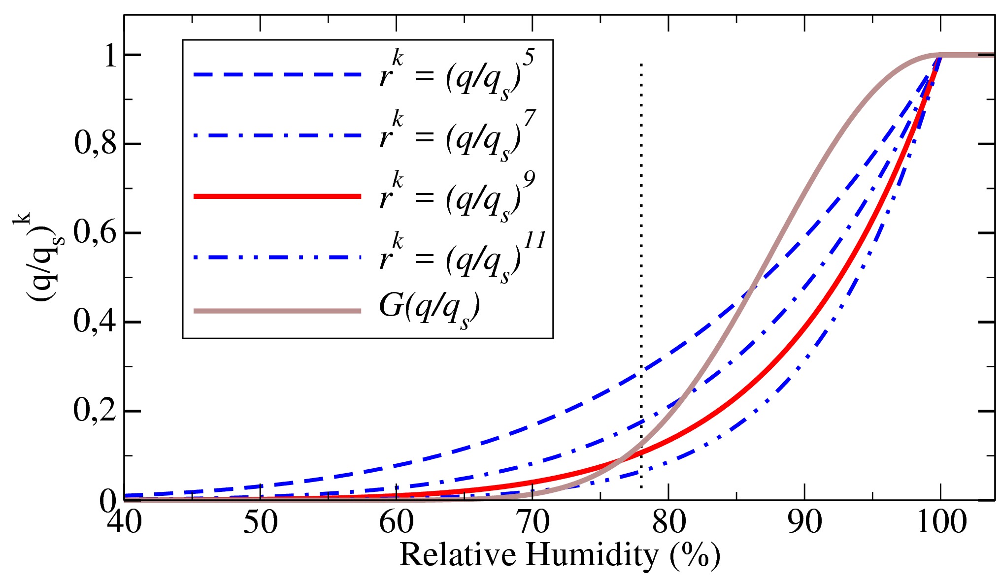 Figure 1
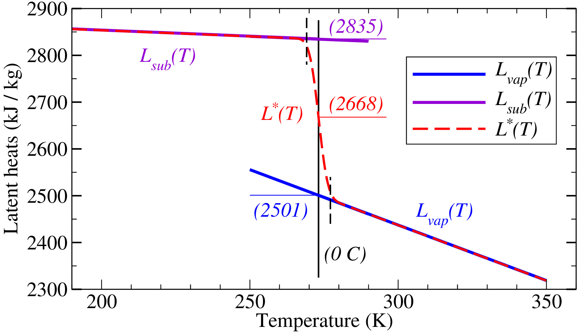 Figure 2
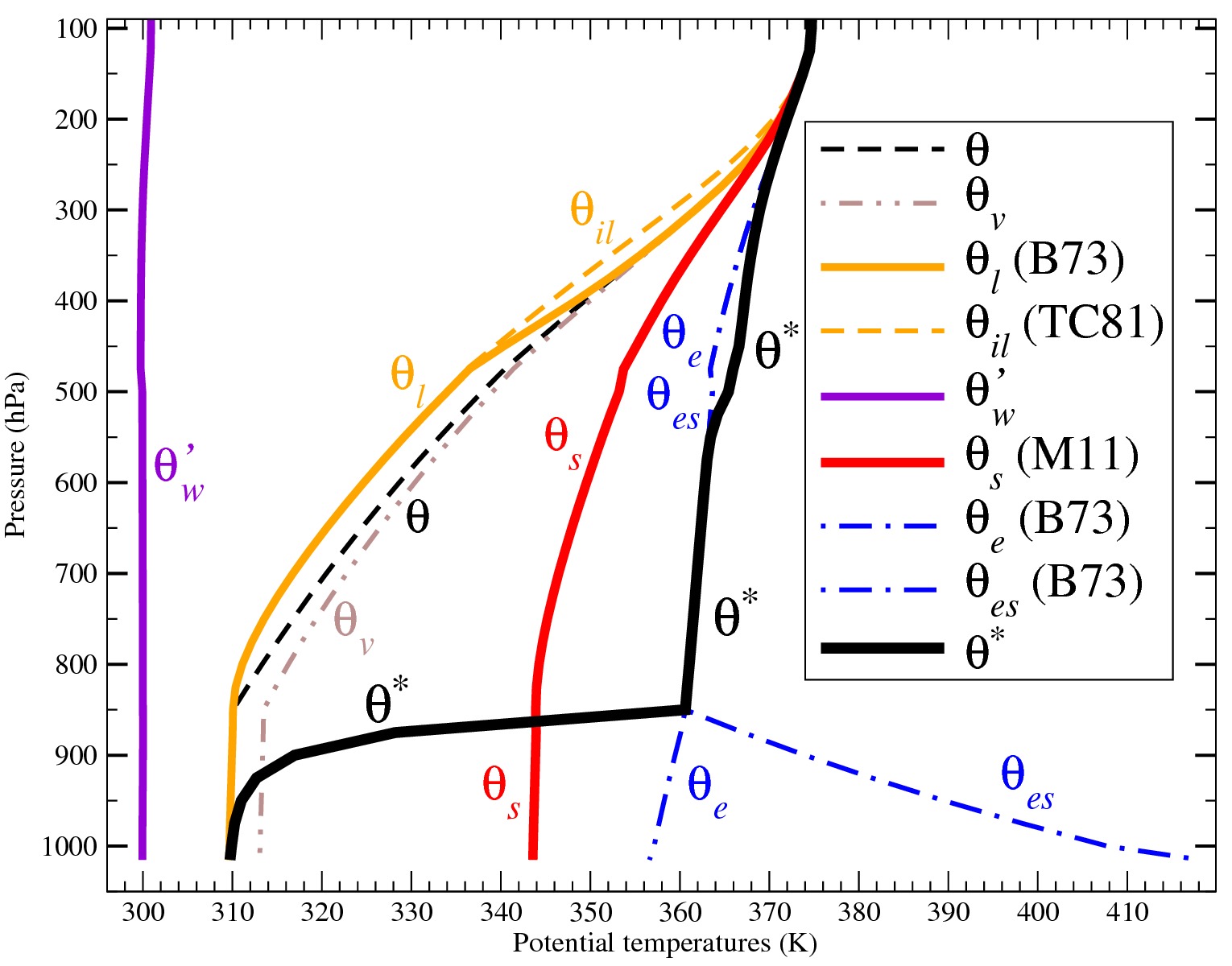 Figure 3
| 1 | 2 | 3 | 4 | 5 | 6 | 7 | 8 | 9 | 10 | 11 | |
|---|---|---|---|---|---|---|---|---|---|---|---|
| 0.78 | 0.61 | 0.48 | 0.37 | 0.29 | 0.23 | 0.18 | 0.14 | 0.11 | 0.08 | 0.07 | |
| 0.75 | 0.56 | 0.42 | 0.32 | 0.23 | 0.18 | 0.13 | 0.10 | 0.08 | 0.06 | 0.04 |
Peer Reviews
No public reviews on file for this paper yet. If you reviewed it on a platform where reviews are public (OpenReview, ICLR, NeurIPS, ICML), you can paste yours below so the community can read it here.
Videos
No videos yet. Explain this paper in a talk, walkthrough, or lecture? Add one.
Taxonomy
Topicsnanoparticles nucleation surface interactions · Fluid Dynamics and Heat Transfer · Icing and De-icing Technologies
Comment on the paper “Generalized dynamic
equations related to condensation and freezing processes” by Wang and Huang (2018).
by Pascal Marquet Météo-France
( March 17, 2024)
*Paper submitted on the 26th of September 2018 to the Journal of Geophysical Research: Atmospheres. *
Corresponding address*: [email protected]*
Partial English translations of 4 Chinese papers of Xing-Rong Wang are provided:
in the Appendix 1 for Wang and Wu (1995)
in the Appendix 2 for Wang, Wang and Shi (1998)
in the Appendix 3 for Wang, Wu and Shi (1999)
in the Appendix 4 for Wang and Wei (2007)
1 The Condensation Probability Function is Arbitrary
A Condensation Probability Function denoted by “” is defined in (Wang and Huang, 2018, hereafter WH18) in accordance with to the previous Chinese papers by Wang and Wu (1995, hereafter WW95) and Wang et al. (1999, hereafter WWS99). This function was defined first as in Eq. (13) of WW95 to conform to the constraints: i) ; and ii) . However, there are many ways for a function to conform to these constraints, and the motivations for the special formulation chosen in WW95 and maintain in WH18 are not clearly exposed. This is a first issue.
Once the arbitrary function had been chosen in WW95, the special value was tuned from Table 1 in WWS99 to conform to the additional constraints: iii) must decrease “sufficiently rapidly” for relative humidities lower than “a certain threshold of %”.
However, the curves of the function , depending on and , are not plotted in WW95, WWS99 or WH18. These curves are plotted in Fig.1, which clearly shows that the requirement iii) is satisfied with any value of between and , but without any criteria given in WWS99 to explain why is the most relevant tuning.
A possible, smoother function, , is plotted in Fig.1 according to
[TABLE]
where . This function has the same properties , and required by WW95 and kept in WH18 with, additionally, for % if the tuning parameter is set to . The additional interesting property is , which means that the null derivative is continuous for %, differently from for small . This property is used in section 3 to derive a smoother version of the potential temperature defined in WH18.
According to all the Chinese and English papers by Xingrong Wang, the aim of introducing the function appears to “eliminate the irrational implicit assumption” that condensation would occur in the atmosphere at the threshold of % of relative humidity. Xingrong Wang explains that he uses the “observational evidence presented by Mason (1971)” that the condensation process may occur at lower values, such as %. However, a careful reading of Mason (1971, p.28-29) reveals that this threshold of only concerns (aerosol) nuclei of pure NaCl hygroscopic salt particles. The same opinion is given in Doswell III (1985, p.31), where it is explained that only the “oceanic salt (resulting when sea spray evaporates in the air)” is hygroscopic and is soluble in water and acts to lower the equilibrium vapor pressure.
Therefore, this threshold of about % cannot be universal throughout the atmosphere, that is to say valid everywhere, at all levels, for all temperatures. The vertical and horizontal distributions of the salt/marine aerosols are highly variable from place to place (Bozzo et al., 2017), making the universal function plotted in Fig.1 unrealistic, since it is the same everywhere in the atmosphere in all papers by Xingrong Wang, including in Gao et al. (2004). In particular, it is likely that the threshold of % must be applied to initiate condensation in mid- and high-tropospheric clouds, where seal-salt aerosols have tiny concentrations.
Another issue is the sentence written in the abstract and the conclusion of the paper by Wang and Feng (2015): the motivation for the introduction of the “Condensation Probability Function” used in WH18 would be “to eliminate the irrational supposition that condensed liquid water always falls immediately”. However, even if it was considered acceptable in the 1980s and 1990s, and maybe up to the mid 2000s, this assumption is no longer made nowadays and the use of prognostic microphysical schemes has become very common, even widespread, in all modern GCM or NWP models.
The authors could have addressed the link between the function and the sub-grid variability of water, as used in all modern GCM and NWP models. The method described first in Sommeria and Deardorff (1977) corresponds to the use of diagnostic (or prognostic) PDF functions to allow the grid cells to generate condensate (liquid water or ice) well before the threshold of % of relative humidity. This method is thus similar to the use of , but the motivations are different, and they do not correspond to the same physical meaning.
2 A Latent Heat Cannot Be Continuous
A new formulation for the latent heat of moist air is suggested in WH18. It is defined by:
[TABLE]
where the right hand side uses more usual meteorological notations: the term is the latent heat of fusion and the term is the latent heat of vaporization . The notation is used in WH18 to represent a freezing probability function defined by a Cumulative Distribution Function, with a tuning parameter determined by the hypothesis: at CC.
The common motivation of all papers by Xingrong Wang since 1995 is to claim that “the latent heat should be continuous”, and that there is a need to “eliminate the irrational assumption” that “condensation only occurs upon saturation”, with a need to “remove the discontinuity” at C. It is indeed possible to write the latent heat for all absolute temperatures by using the discontinuous Heaviside step function if C and otherwise, leading to
[TABLE]
A comparison of Eqs.(2) and (3) shows that is replaced by in WH18. The smooth transition of between and is indeed visible in Fig.2, where is plotted from Eq.(2).
However, the arguments of Xingrong Wang are based on a misleading interpretation of the latent heat, which cannot be continuous, since the latent heats are precisely defined in thermodynamics as the differences in enthalpies for two different states of water, with obvious discontinuities at C between liquid water and ice. This means that the two latent heats and precisely take these discontinuities into account, and they cannot be somehow interpolated by a smooth function like .
Moreover, the use, in WH18, of the temperature of about C, at which the density of water is maximum, seems artificial for defining , because a latent heat depends only on the difference in enthalpies and is independent of the density of the species. The use of this temperature of about C corresponds to the strange impacts shown in Fig.2: decreases for C, increases for C and kJ/kg at C. All these results disagree with basic results of the thermodynamics of moist air.
3 The New Potential Temperature Introduces Discontinuities
A new potential temperature is defined in WW18 by:
[TABLE]
where , is the saturating value of the specific content , and is given by Eq. (2). A certain updraft of a mixed-phase cumulus is used to compute and plot most of the existing potential temperatures in Fig.3, including the new one .
The saturated equivalent potential temperature derived in Betts (1973) is a special case of if and , and the equivalent potential temperature can be obtained by replacing the saturating value by the water vapor value . The liquid-water potential temperature is defined in Betts (1973), the virtual potential temperature in Lilly (1968), the ice-liquid formulation in Tripoli and Cotton (1981) and the entropy potential temperature in Marquet (2011, 2017).
All the potential temperatures , , , , and are almost constant in the boundary layer below the condensation level, whereas increases slightly with height due to the term , which increases for decreasing values of (see Fig.2). This is not the case for and , which both exhibit intriguing features in the boundary layer.
On the one hand, the saturating value decreases very rapidly with height, by about K between and hPa, due to the large decrease of with . On the other hand, the new potential temperature increases rapidly with height, by about K, for this very moist and warm tropical profile. It follows that gradually switches from the small, surface values of toward the large values of at the condensation level. This strange feature observed for is a consequence of at the condensation level, thus with , and with for lower relative humidities, thus with close to the surface.
The potential temperatures , and possess clear physical meanings, since they correspond to pseudo-adiabatic processes, buoyancy force and entropy state function, respectively. Similarly, and are adiabatic quantities that are conserved if is a constant. In contrast, the switch of between and is proof that cannot be related to any of these properties, and cannot have a clear physical meaning.
Moreover, this rapid increase of and in the boundary layer corresponds to a large vertical gradient and, therefore, must have large impact on the values of the potential vorticity defined by in WH18. This large impact of the term on the definition of and in the boundary layer is neither shown nor discussed in WH18.
Lastly, the impact of at the saturation level leads to a paradoxical issue: is introduced in WH18 to “remove certain discontinuities”, although there is clearly a new discontinuous change in the gradient at the condensation level in Fig.3. This discontinuity of the derivative of at is obvious in Fig.1 at % and is explained by the derivative and for small . This strange feature is shared only with and must greatly impact both and . This discontinuity can be removed by choosing the arbitrary function invented for this Comment, plotted in Fig.1 and given by Eq.(1) with .
The reference list from the paper itself. Each links out to its DOI / PubMed record.
- 1Betts (1973) Betts, A. K., 1973: Non-precipitating cumulus convection and its parameterization. Q. J. R. Meteorol. Soc. , 99 (419) , 178–196, doi: 10.1002/qj.49709941915 .
- 2Bozzo et al. (2017) Bozzo, A., S. Rémy, A. Benedetti, J. Flemming, P. Bechtold, M. Rodwell, and J.-J. Morcrette, 2017: Implementation of a CAMS-based aerosol climatology in the IFS. Technical memorandum of ECMWF. Number 801.
- 3Doswell III (1985) Doswell III, C. A., 1985: The Operational Meteorology of Convective Weather. Volume 2. Storm Scale Analysis (252 pp.) . NOAA Technical Memorandum, ESG-15, Environmental Research Laboratories, 252 pp.
- 4Gao et al. (2004) Gao, S., X. Wang, and Y. Zhou, 2004: Generation of generalized moist potential vorticity in a frictionless and moist adiabatic flow. Geophys. Res. Lett. , 31 (12) , L 12 113, doi: 10.1029/2003 GL 019152 .
- 5Lilly (1968) Lilly, D. K., 1968: Models of cloud-topped mixed layers under a strong inversion. Quart. J. Roy. Meteor. Soc. , 94 (401) , 292–309, doi: 10.1002/qj.49709440106 .
- 6Marquet (2011) Marquet, P., 2011: Definition of a moist entropy potential temperature: application to FIRE-I data flights. Quart. J. Roy. Meteor. Soc. , 137 (9) , 768–791, doi: 10.1002/qj.787 , URL http://arxiv.org/abs/1401.1097 .
- 7Marquet (2017) Marquet, P., 2017: A third-law isentropic analysis of a simulated hurricane. J. Atmos. Sci. , 74 (10) , 3451–3471, doi: 10.1175/JAS-D-17-0126.1 , URL https://arxiv.org/abs/1704.06098 .
- 8Mason (1971) Mason, B. J., 1971: The physics of clouds (671 pp.) . Oxford, Oxford University Press, 671 pp.