TL;DR
icet is a versatile Python library that streamlines the construction, sampling, and analysis of alloy cluster expansions, facilitating integration with first-principles calculations and machine learning for materials modeling.
Contribution
The paper introduces icet, a flexible and efficient Python package for building and sampling alloy cluster expansions, with extensive features for regression, validation, and data management.
Findings
Successful computation of a metallic alloy phase diagram
Analysis of chemical ordering in an inorganic semiconductor
Demonstration of icet's integration with first-principles and ML tools
Abstract
Alloy cluster expansions (CEs) provide an accurate and computationally efficient mapping of the potential energy surface of multi-component systems that enables comprehensive sampling of the many-dimensional configuration space. Here, we introduce \textsc{icet}, a flexible, extensible, and computationally efficient software package for the construction and sampling of CEs. \textsc{icet} is largely written in Python for easy integration in comprehensive workflows, including first-principles calculations for the generation of reference data and machine learning libraries for training and validation. The package enables training using a variety of linear regression algorithms with and without regularization, Bayesian regression, feature selection, and cross-validation. It also provides complementary functionality for structure enumeration and mapping as well as data management and…
Click any figure to enlarge with its caption.
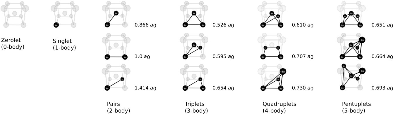 Figure 1
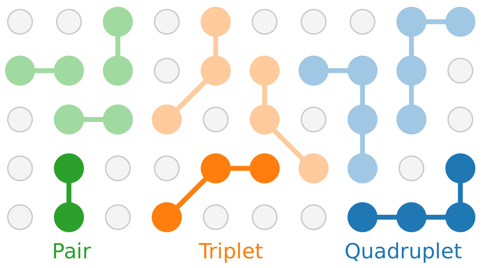 Figure 2
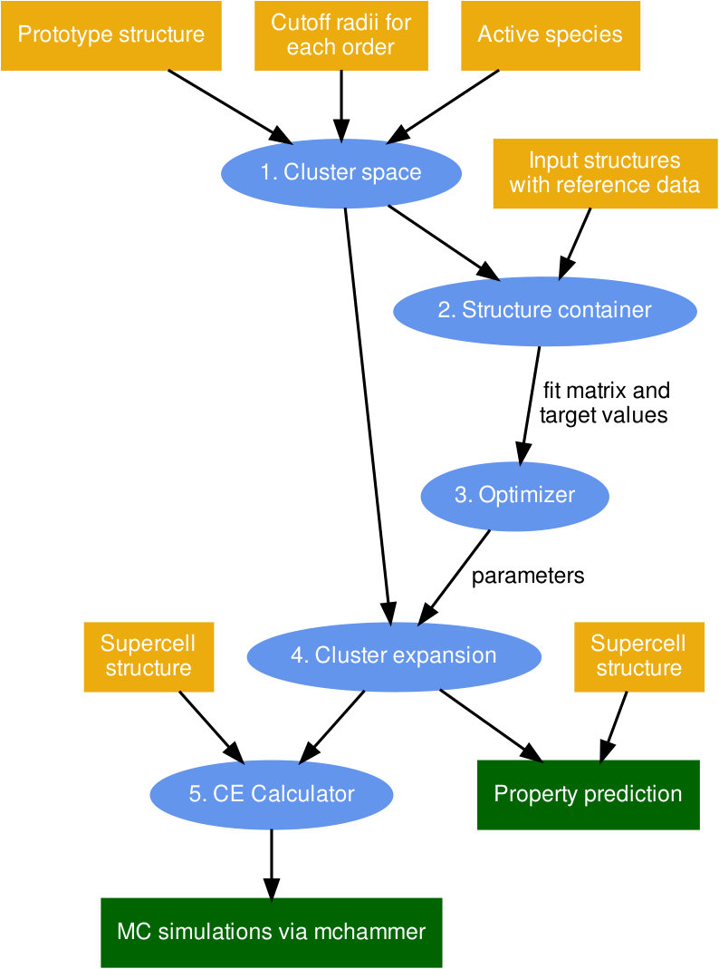 Figure 3
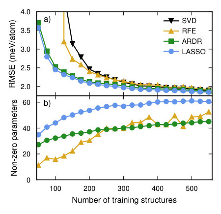 Figure 4
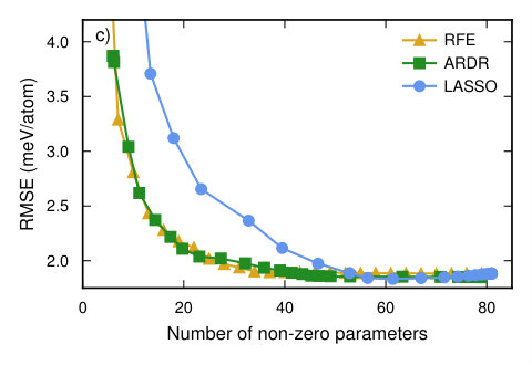 Figure 4
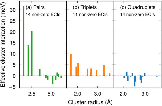 Figure 5
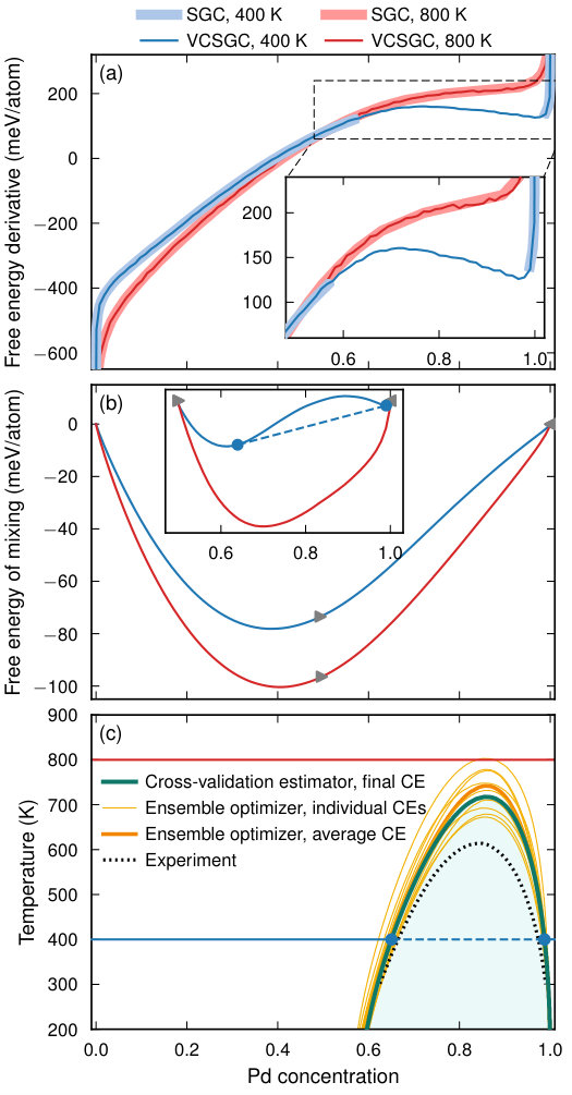 Figure 6
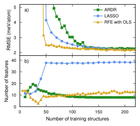 Figure 7
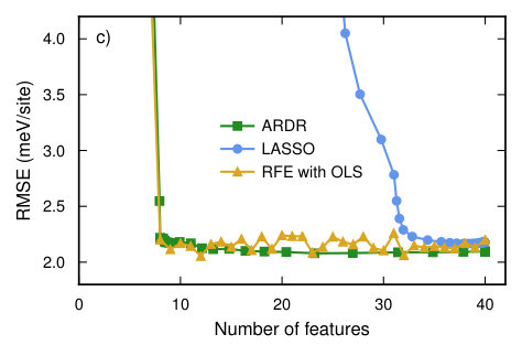 Figure 7
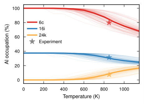 Figure 8
Peer Reviews
No public reviews on file for this paper yet. If you reviewed it on a platform where reviews are public (OpenReview, ICLR, NeurIPS, ICML), you can paste yours below so the community can read it here.
Code & Models
Videos
No videos yet. Explain this paper in a talk, walkthrough, or lecture? Add one.
icet – A Python library for constructing and sampling alloy cluster expansions
Mattias Ångqvist
William A. Muñoz
J. Magnus Rahm
Erik Fransson
Chalmers University of Technology, Department of Physics, Gothenburg, Sweden
Céline Durniak
Piotr Rozyczko
Thomas Holm Rod
Data Management and Software Centre, European Spallation Source, Copenhagen, Denmark
Paul Erhart
Chalmers University of Technology, Department of Physics, Gothenburg, Sweden
Abstract
Alloy cluster expansions (CEs) provide an accurate and computationally efficient mapping of the potential energy surface of multi-component systems that enables comprehensive sampling of the many-dimensional configuration space. Here, we introduce icet, a flexible, extensible, and computationally efficient software package for the construction and sampling of CEs. icet is largely written in Python for easy integration in comprehensive workflows, including first-principles calculations for the generation of reference data and machine learning libraries for training and validation. The package enables training using a variety of linear regression algorithms with and without regularization, Bayesian regression, feature selection, and cross-validation. It also provides complementary functionality for structure enumeration and mapping as well as data management and analysis. Potential applications are illustrated by two examples, including the computation of the phase diagram of a prototypical metallic alloy and the analysis of chemical ordering in an inorganic semiconductor.
I Introduction
Ordering phenomena are ubiquitous in materials science, physics, and chemistry. They are particularly relevant in multi-component systems, where they are associated for example with phase transitions, segregation as well as chemical order Van der Ven et al. (2018). The underlying energetics can usually be assessed by first-principles calculations, based on e.g., density functional theory (DFT), with good accuracy. The computational cost of such calculations, however, precludes a statistically adequate sampling of the relevant configuration space. In this context, alloy cluster expansions (CEs) in combination with Monte Carlo (MC) simulations provide a powerful means to balance computational efficiency and accuracy Sanchez et al. (1984); de Fontaine (1994).
The CE approach has been widely and very successfully adopted to analyze for example phase diagrams in metallic Asta et al. (1993); Ozoliņš et al. (1998) and semiconducting alloys Van der Ven et al. (1998); Ceder et al. (2000); Zhou et al. (2006), including surfaces Drautz et al. (2001); Sluiter and Kawazoe (2003); Welker et al. (2010); Stephens et al. (2010); Chen et al. (2011); Cao and Mueller (2015); Herder et al. (2015) as well as nanoparticles Mueller and Ceder (2010); Chepulskii et al. (2010); Yuge (2011); Mueller (2012); Tan et al. (2012); Wang et al. (2014); Li et al. (2018); Cao et al. (2018). CEs have also been applied to study the temperature and composition dependence of ordering in various materials Kim et al. (2010); Ångqvist et al. (2016); Ångqvist and Erhart (2017); Troppenz et al. (2017); Gunda et al. (2018). The CE approach is not limited to the mapping of total and mixing energies but can also be applied to model for example activation barriers Van der Ven et al. (2001), vibrational properties Morgan et al. (2000); van de Walle and Ceder (2002a), chemical expansion Ångqvist and Erhart (2017), or transport properties Ångqvist et al. (2016).
Here, we introduce the integrated cluster expansion toolkit (icet) to enable efficient construction and sampling of CEs. icet is designed to be modular, extensible, and flexible, while maintaining high computational efficiency. This enables integration of icet in extended workflows, reflecting the ongoing shift toward machine learning and large data initiatives in computational material science Taylor et al. (2014); Pizzi et al. (2016). icet is primarily developed in Python whereas computationally more demanding parts are written in C++, providing performance while maintaining portability and ease-of-use. This approach enables easy integration for example with countless first-principles codes and analysis tools accessible via the atomic simulation environment (ase) Larsen et al. (2017) as well as state-of-the-art regression techniques via scikit-learn Pedregosa et al. (2011).
icet provides a feature set that is comparable to or extends beyond earlier monolithic codes, such as the ATAT van de Walle and Ceder (2002b); van de Walle (2009); van de Walle and Asta (2002), the UNCLE Lerch et al. (2009) or CASM codes cas (1 10). Since icet is written in Python, it is, however, straightforward to add new functionality. This enables one for example to implement advanced algorithms for finding ground states Huang et al. (2016); Larsen et al. (2018). icet is available under an open-source license and hosted on gitlab to encourage community participation. Current functionality includes for example:
- •
support for multiple species and multiple coexisting sub-lattices, e.g., Ba8-xSrxGayGe46-y or Au1-xPdx:Hy
- •
advanced linear regression techniques with regularization (including compressive sensing Nelson et al. (2013a)), cross-validation, and ensemble optimization via scikit-learn Pedregosa et al. (2011)
- •
MC simulations in various ensembles using observers and multiple CEs in parallel via the mchammer module
- •
supplemental functionality including e.g., structure enumeration Hart and Forcade (2008, 2009), structure mapping, convex hull extraction Barber et al. (1996), and ground state finding Larsen et al. (2018)
The remainder of this paper is organized as follows. The next section describes the methodologies implemented in icet, including an overview of the CE formalism, algorithms available for CE construction, and the mchammer module for sampling CEs via MC simulations. The components and workflow of icet are summarized in Sect. V. Section VI demonstrates the potential of icet via examples. The first example addresses the construction and sampling of CEs for the Ag–Pd system as well as the subsequent generation of a phase diagram from these data. The second example summarizes the application of icet for the simulation of chemical ordering in a semiconducting system, specifically an inorganic clathrate.
II Cluster expansion formalism
II.1 Clusters and orbits
The objective of a CE is to describe the variation of a property of interest, most commonly the energy, with the chemical configuration, i.e. the distribution of different species over a lattice. To this end, the structure is decomposed into a set of clusters, where a cluster of order is defined as a list of sites. Clusters are commonly referred to by order as singlets, pairs, triplets and so on.
The clusters are subject to the symmetry of the underlying lattice, as described by the associated space group (for periodic systems) or point group (for non-extended systems). Clusters that can be mapped onto each other as a result of the application of an intrinsic symmetry operation of the lattice, are said to belong to the same orbit (Fig. 2). Each orbit in turn is represented by a symmetry inequivalent cluster, from which every other cluster of the orbit can be generated by application of the symmetry operations and a permutation of the sites.
While the number of clusters is in principle infinite, the short-ranged nature of physical interactions implies that clusters with notable contributions to the CE are commonly shorter-ranged and few-bodied. It is therefore customary to only include clusters up a certain size and order, as shown for the case of a BCC lattice in Fig. 1.
II.2 Point functions
It can be formally shown that a CE is able to represent any function of the configuration if one can construct a complete orthogonal basis Sanchez et al. (1984). Here, denotes the occupation vector, the elements of which indicate the species that resides on the corresponding site. To obtain a practical procedure, for each lattice point one can define orthogonal point functions
[TABLE]
where is the allowed number of species and goes from 0 to . These point functions form an orthogonal set over all possible occupation numbers van de Walle (2009),
[TABLE]
In the case of multiple sublattices can assume different values for different sublattices. For example, in the case of the zincblende alloy Al1-x-yGaxInyAs1-zSbz, for the cation and for the anion lattice.
II.3 CE expression
A set of functions in the -dimensional configuration space can now be constructed as products of point functions,
[TABLE]
Here, , where are point function indices and is the number of sites in the structure. Each corresponds to a cluster in the sense that if site is not part of the cluster (such that the corresponding point function is ) and nonzero otherwise. In the binary case, there is one for each cluster, each having elements that are either 0 or 1. In systems with more than two components, there are multiple corresponding to the same cluster, due to the the possible combinations of nonzero point function indices .
It can be shown that the functions form a complete orthogonal set, so that any function of the configuration can be expressed as
[TABLE]
All basis functions have one configuration invariant component that is equal to 1 when . One can therefore omit the latter from the basis functions and instead use one configuration invariant term . Furthermore, taking into account the symmetry of the clusters the summation can be carried out over orbits (or representative clusters) rather than all clusters, which yields the full CE expression
[TABLE]
The bracket indicates the average over the basis functions for all that are symmetry equivalent to . The effective cluster interactions (ECIs) are the free parameters of the CE and the target of the training procedure described in the next section. Finally, denotes the multiplicity of the representative cluster .
III Cluster expansion construction
III.1 Matrix form
To obtain a CE for a specific material one must determine the ECIs. To this end, one requires reference data in the form of a set of configurations as well as an associated vector of target data , which is usually obtained from first-principles calculations. Equation (1) can be cast in the form
[TABLE]
where the rows of are given by
[TABLE]
and denotes the ECIs with . Note that it can sometimes be useful to exclude from and let the target values refer to the primitive unit cell. This will ensure all elements in are in the interval and avoids a bias due to the number of elements in .
III.2 Linear regression techniques
Following the decomposition of a lattice into clusters and the construction of the sensing matrix, it remains to determine the ECIs by solving the linear system given by Eq. (2). This is equivalent to finding the parameter vector that minimizes . In principle a solution can be determined by conventional least-squares, which works well in the overdetermined limit. Due to the computational cost associated with DFT calculations the linear system is, however, often underdetermined and/or rows of the sensing matrix are correlated. At the same time, the nearsightedness of physical interactions suggests that the solution vector be sparse Nelson et al. (2013a). We are thus faced with the task of feature selection, a common process in machine learning, which yields models that are less prone to overfitting and more transferable. It can also reduce the computational expense during sampling (see Sect. IV).
To achieve sparse solutions and combat overfitting one can include regularization terms in the objective function in the form of the or -norm of the solution vector. Consider, for example, elastic net regularization, for which
[TABLE]
For this expression reduces to Ridge regression while for one obtains the expression commonly used for solving the least absolute shrinkage and selection operator (LASSO) problem. Other techniques include the split-Bregman algorithm, which has been previously used for constructing CEs Nelson et al. (2013a), as well as recursive feature elimination (RFE), which iteratively removes the weakest parameters from a model and can be applied to different objective functions. Furthermore, there are Bayesian linear regression techniques such as automatic relevance detection regression (ARDR), which provide probabilistic models of the regression problem at hand, and Bayesian compressive sampling Nelson et al. (2013b). The parameters that are intrinsic to a regression algorithm, such as in the case of LASSO or the allowed number of features in the case of RFE, are known as hyper-parameters.
The performance of different models can be assessed by cross-validation (CV). To this end, the available reference data is split into training and validation sets. The former is used to fit a model, whereas the latter is used to measure the predictive power of the model, usually via the root-mean-square error (RMSE)
[TABLE]
where the summation extends over the structures comprising the validation set. To reduce the statistical error, the RMSE is furthermore averaged over several different splits of the reference data.
icet supports various regression techniques, including the ones named above, via the scikit-learn machine learning library Pedregosa et al. (2011) and allows one to compute CV scores in a number of different ways. Since sensing matrix and target data are readily available via the Python interface, one can also interface directly with scikit-learn or other machine learning libraries. icet also provides functionality for generating ensembles of models from a single sensing matrix. Thereby it is possible to check the sensitivity and stability of more advanced prediction, as illustrated in the examples below.
IV Cluster expansion sampling
A CE can be employed in a number of different ways, including finding ground states Larsen et al. (2018), but it is most commonly sampled using MC simulations. For this purpose, icet includes the mchammer module, which supports various thermodynamic ensembles and provides supplemental functionality for data management and analysis.
MC sampling is carried out using the Metropolis algorithm, in which a trial is accepted with probability
[TABLE]
Here, and is the change in the thermodynamic potential associated with the ensemble being sampled (excluding the entropy term).
In the case of the canonical () ensemble the thermodynamic potential equals the internal energy, , and a trial step involves swapping the species of two sites (conserving the concentrations).
Especially when exploring phase diagrams it is often useful to sample along the concentration axes. This can be achieved for example by using the semi-grand canonical (SGC) () ensemble. In this case, the trial move involves only one site, for which the occupation is swapped and the underlying thermodynamic potential is , where is the total number of sites, is the concentration of species , and the chemical potential difference of species relative to the first species.
In the SGC ensemble the mapping from chemical potential difference to concentration is multi-valued in two-phase regions. It therefore cannot be used to sample across miscibility gaps. This shortcoming can be overcome by employing the variance-constrained semi-grand canonical (VCSGC) ensemble Sadigh and Erhart (2012), which uses the same trial move as the SGC ensemble but for which . The intensive parameters and constrain respectively the average and the fluctuation of the concentration.
The choice of ensemble is motivated by the characteristics of the system and the objective of the simulations. The canonical ensemble conserves concentrations, which makes it ideal for studying systems at specific compositions, extracting structural order parameters or obtaining ground states by simulated annealing. The SGC and VCSGC ensembles, on the other hand, allow the composition to be continuously varied and by extension the integration of the free energy. In the SGC ensemble, the concentration derivative of the canonical free energy is given (for simplicity for a binary system) by
[TABLE]
This relation is, however, useful only in single-phase regions of the phase diagram, where maps to one and only one concentration. In SGC simulations, multi-phase regions manifest themselves by discontinuous jumps between phase boundaries. Such discontinuities, if carefully studied, can be exploited for tracking phase boundaries but hinder integration of the free energy van de Walle and Asta (2002).
In the VCSGC ensemble, the canonical free energy derivative is (for a sufficiently large system) given by Sadigh and Erhart (2012)
[TABLE]
where is the average observed concentration. Unlike the SGC ensemble, the mapping between and concentration is always one-to-one for a sufficiently large value of , whence the free energy can be recovered by integration across multi-phase regions. The phase diagram can then be constructed with standard techniques for free energy minimization.
MC simulations in both the SGC and VCSGC ensembles are illustrated in Sect. VI.1 whereas the canonical ensemble is employed in Sect. VI.2.
V Workflow
icet integrates the CE formalism (Sect. II) with linear regression (Sect. III) and sampling techniques (Sect. IV) into one workflow (Fig. 3). Assuming reference data, say from DFT calculations, is available for a set of structures that have been generated for example by enumeration Hart and Forcade (2008) the construction and sampling of a CE proceeds as follows.
The first step involves constructing a cluster space, which requires a prototype structure, a set of cutoff radii that define which clusters to include in the expansion, and a specification as to which species are allowed on each site. Internally, the spglib library Togo and Tanaka (2018) is employed to find the symmetries of the underlying lattice. 2. 2.
Next, cluster vectors are computed according to Eq. (3) for all structures in the reference set and compiled into a structure container, which holds the sensing matrix as well as the vector of target values . 3. 3.
Then linear regression techniques in combination with CV are employed to solve Eq. (2) and find an optimal parameter vector . Here, externally provided optimization algorithms from, e.g., scikit-learn and scipy can be used. 4. 4.
Parameters and cluster space are subsequently combined to obtain the actual CE, which can be used to predict the property in question for arbitrary supercells of the prototype structure. 5. 5.
For efficient sampling one can also set up a CE calculator for a specific supercell to be used in MC simulations via the mchammer module.
This workflow is supplemented by a number of tools, which enable one for example to enumerate structures Hart and Forcade (2008), extract the convex hull, map relaxed structures onto ideal lattices, or find ground states Larsen et al. (2018).
A full description of the different entities involved in this process and the Python objects that describe them can be found in the icet user guide ice (1 10).
VI Applications
VI.1 Phase diagram of the Ag–Pd system
VI.1.1 Reference calculations
As a first example for the application of icet, we describe the construction of a CE for the face-centered cubic (FCC) Ag–Pd alloy. To this end, a database of 631 reference structures corresponding to all distinct supercells with up to 8 atoms was set up using the structure enumeration feature of icet. More refined structure selection approaches are available Nelson et al. (2013a) but are not considered in this example.
Reference calculations were then carried out using DFT calculations using the projector augmented method Blöchl (1994); Kresse and Joubert (1999) as implemented in vasp Kresse and Furthmüller (1996a, b). The van-der-Waals density functional method Dion et al. (2004); Klimes̆ et al. (2011) with consistent exchange Berland and Hyldgaard (2014), which has been shown to be very well suited for transition metals Gharaee et al. (2017), was employed to represent the exchange-correlation potential. The Brillouin zone was sampled using -point grids equivalent to a -mesh for the primitive FCC unit cell and the plane wave cutoff energy was set to 384 eV. Both the atomic positions and the cell metric were relaxed until residual forces and stress were less than 10 meV/Å and 0.8 GPa, respectively. Relaxations were carried out using first-order Methfessel-Paxton smearing with a width of 0.1 eV. Final energy calculations were carried out using for the relaxed structures the tetrahedron method with Blöchl corrections using a smearing width of 0.05 eV.
VI.1.2 Construction of CE models
Next a cluster space was set up, including clusters up to fourth order with cutoffs of 3.3 , 1.6 , and 1.5 in units of the lattice parameter for pairs, triplets, and quadruplets, respectively. The resulting cluster space contained 81 parameters, including 1 zerolet, 1 singlet, 24 pairs, 20 triplets, and 35 quadruplets. In principle, icet does not impose limits on cluster order or size.
In order to study the convergence with respect to the number of training structures we computed the learning curve using the RMSE score averaged over the validation set using the CV estimator functionality in icet. The latter generates an estimate for the CV-RMSE score by using the shuffle-split method with 50 splits, while the final CE is obtained by training against the complete data set. Four different optimization methods were compared, including singular value decomposition, LASSO, RFE based on ordinary least-squares (OLS), and ARDR (Fig. 4a).
In the overdetermined region all methods yield similar CV-RMSE scores; in the underdetermined region, though, LASSO and ARDR outperform the other two methods. While LASSO and ARDR have almost identical CV scores there is, however, a significant difference in the number of features, i.e. non-zero parameters (Fig. 4b). To study this behavior further we analyzed the CV-RMSE score as a function of the number of features in the solution (Fig. 4c). To this end, we used a training set of 563 structures and scanned the hyper-parameters of the regression algorithms to control the sparsity of the solution.
This analysis reveals that ARDR and RFE with OLS yield CEs with a very low CV-RMSE of 2 meV/atom using only 30 features. LASSO reaches the same level but yields about 50 features. In this case, ARDR is thus the method of choice since it converges as quickly with the number of training structures as LASSO but yields a smaller number of orbits with non-zero ECIs (Fig. 5), which leads to a more transferable model and reduces the computational cost for sampling.
VI.1.3 Phase diagram from MC simulations
To construct a phase diagram for the Ag–Pd system, we employed the mchammer module for sampling a conventional FCC supercell (500 sites) in both the SGC and VCSGC ensembles. We carried out 200,000 MC trial steps with the SGC ensemble at 105 values of in the range and the same number of trial steps with the VCSGC ensemble at and 105 values of in the range . Simulations were run at 25 K intervals between 100 and 900 K, corresponding in total to approximately trial steps or MC cycles.
Simulations were first carried out for the CE described above that was constructed using the CV estimator with ARDR and the full dataset of 631 structures (CV-RMSE 2 meV/atom).
The free energy derivatives extracted from the SGC and VCSGC simulations (using Eqs. (4) and (5)) coincide everywhere except for a region on the Pd-rich side at lower temperatures where the SGC simulations exhibit a discontinuity, which is the hallmark of a two-phase region (Fig. 6a). In this situation, the full free energy can thus only be recovered from the VCSGC simulations (Fig. 6b). The two-phase region is manifested by a concave region in the free energy of mixing (inset in Fig. 6b).
To construct the phase diagram, we fitted the free energy of mixing Fig. 6b) to third-order Redlich–Kister polynomials at each temperature separately and then fitted the temperature dependence of the polynomial expansion coefficients to conventional third-order polynomials. This representation provides a continuous and smooth map of the free energy in both temperature and composition, akin to the CALPHAD approach Dinsdale et al. (2008). The predicted phase diagram exhibits a pronounced miscibility gap on the Pd-rich side with a critical temperature of 718 K. This is overall in good agreement with the experimental result Dinsdale et al. (2008), except for an overestimation of , which has been experimentally determined as approximately 610 K.
To illustrate the sensitivity of the phase diagram to variations in the training set, we also considered a set of ten CEs that were obtained using the ARDR method via the ensemble optimizer functionality of icet. The latter approach enables one to generate a series of CEs that are trained in identical fashion but are based on different training sets. The latter are generated by selection with replacement (bagging) from the reference data set such that the number of structures in the training sets equals the number of reference structures. The thus obtained CEs are numerically very similar to the CE obtained using the CV estimator approach before (Fig. 4). Using this set of CEs enabled us to estimate not only the error in the mixing energies but its impact on the final phase diagram.
The CE obtained by averaging the ECIs over all CEs in the ensemble yields a of 742 K that is only slightly higher than the CE generated using the CV estimator. The individual CEs yield, however, a larger variation, spanning the range from 673 to 803 K. This demonstrates that CV-RMSE alone is an insufficient measure of the quality of a CE. Rather a more careful assessment of the quantity of interest must be carried out if an accurate estimate is required.
VI.2 Chemical ordering in an inorganic clathrate
VI.2.1 Background and reference structures
The CE approach is not limited to metallic system and the prediction of phase diagrams. It is also very useful to model for example the degree of ordering as a function of temperature and composition. The latter can in turn can be experimentally assessed using diffraction techniques based on X-ray or neutron scattering Christensen et al. (2010). Here, this possibility is illustrated by using icet to predict the site occupancy factors (SOFs) in the inorganic clathrate Ba8AlxSi46-x.
Clathrates are inclusion compounds with a lattice structure that can trap atomic or small molecular species. Ba8AlxSi46-x falls into the class of type-I clathrates, which belong to spacegroup Pmn.Shevelkov and Kovnir (2011) In this case, the host lattice is made up of Al and Si atoms, which occupy Wyckoff sites , , and , whereas Ba atoms reside inside the cages for charge balance. Al and Si do not occupy the framework sites randomly but exhibit some degree of ordering, which results from a delicate balance between energy and entropy and can be experimentally accessed via the SOFs. While for a completely random distribution at, e.g., one would expect SOFs of 12/46=26% for all sites, in Ba8AlxSi46-x one observes values in the range from close to zero to 80% Roudebush et al. (2012). Detailed studies of this behavior, including careful comparison with experiment, have been published elsewhere Ångqvist et al. (2016); Ångqvist and Erhart (2017); Troppenz et al. (2017). Here, we focus on the construction and sampling of CEs for this system, in particular highlighting the analysis capabilities provided by icet.
VI.2.2 CE construction
The unit cell contains 46 framework sites, which prevents an enumeration approach for structure generation. Instead, 240 occupations of the primitive unit cell for were produced by randomly distributing Al and Si atoms over the host lattice. The structures were relaxed using DFT calculations using a similar procedure as for the Ag–Pd structures described above. The PBE exchange-correlation functional was used Perdew et al. (1996) with a plane wave energy cutoff of 319 eV and a -centered -point mesh. The other parameters were identical to those given in Sect. VI.1.
A cluster basis was constructed using a cutoff of 0.49 for both pairs and triplets, resulting in 13 and 23 symmetry inequivalent clusters, respectively. CEs were generated using ARDR, LASSO, and RFE with OLS in conjunction with the CV estimator functionality based on the shuffle-split method with 50 splits.
RFE with OLS yields both fast convergence with training set size and sparse solutions (Fig. 7a,b). LASSO and ARDR require almost twice as many training structures to achieve similar CV-RMSE values. ARDR provides sparse solutions that are similar to those obtained by RFE with OLS. The CE models obtained by LASSO, however, have a much larger number of features (Fig. 7c). These trends are similar to the case of Ag–Pd (Sect. VI.1) except for the roles of ARDR and RFE with OLS being reversed.
VI.2.3 CE sampling
To predict the SOFs as a function of temperature, we employed the mchammer module for sampling a supercell (268 sites) in the canonical ensemble at , for which experimental data is available Roudebush et al. (2012), using a simulated annealing approach. The temperature was decreased from 1200 to 0 K at a rate of 100 K/10,000 MC cycles, corresponding to a total of almost 48 million trial steps. The SOFs were monitored during the simulation using the observer functionality of icet, which enables one to compute various quantities of interest at specified intervals along the trajectory.
The simulations were first carried out using the CE obtained using RFE with OLS and a set of 240 structures. To estimate the statistical reliability of the thus predicted SOFs, we furthermore ran the simulations for an ensemble of models that were generated from the available data (bagging), in almost identical fashion as for the Ag–Pd models described above.
At the composition of the number of nearest neighbor Al–Al pairs is zero over the entire temperature range. This behavior is due to Al–Al bonds being energetically unfavorable, which is familiar from the Loewenstein rule for zeolites. While the Al–Al pair distribution is experimentally practically impossible to access, diffraction experiments can provide information about the SOFs, which are ultimately the result of the interplay of energy and entropy Christensen et al. (2010). The SOFs obtained from MC simulations exhibit a systematic variation with temperature and strongly deviate from the random limit, which would correspond to approximately 35% (Fig. 8). At temperatures below approximately 600 K the SOFs converge and the structure adopts a well ordered configuration. The ground state at this stoichiometry corresponds to Al SOFs of 100%, 37.5%, and 0% for Wyckoff sites 6c, 16i, and 24k, respectively, in agreement with earlier simulations Ångqvist and Erhart (2017); Troppenz et al. (2017).
The calculated SOFs compare very well with the available experimental data in the temperature interval between 800 and 900 K Roudebush et al. (2012). This is very reasonable since it is likely that kinetic factors prevent full ordering in the experiments. A more extensive analysis of the SOFs as both a function of temperature and composition Ångqvist and Erhart (2017) shows very good comparison with experiment over the entire composition range Christensen et al. (2010); Roudebush et al. (2012), which further validates the present approach. The ground state configurations obtained in the zero-temperature limit are valuable in themselves as they provide ordered prototypes, which can be used for further analyses of e.g., electrical Ångqvist et al. (2016) and thermal transport properties Lindroth et al. (2019).
VII Conclusions
In the present paper, we have introduced the icet Python package for the construction and sampling of alloy CEs. Thanks to its modular design it can be readily extended and combined with other Python packages to achieve complex functionalities. It thereby also provides an excellent environment for method development, including the adaptation of further machine learning techniques (e.g., genetic algorithms Blum et al. (2005)) and the integration in extended workflows, e.g., in the context of high-throughput computing Taylor et al. (2014); Pizzi et al. (2016). icet also provides a number of supplementary features pertaining, e.g., to structure enumeration and mapping as well as data analysis.
icet readily supports a variety of different methods for constructing CEs, as demonstrated specifically for the metallic alloy Ag–Pd and the inorganic clathrate Ba8AlxSi46-x. Several different regression methods were compared, illustrating a balance between the sparsity of the solution and the accuracy of the final CE. While for Ag–Pd the ARDR method provided the best performance, yielding both low CV scores and a sparse solution, RFE based on OLS achieved the best results in the case of Ba8AlxSi46-x. Regression using LASSO led to less optimal solutions in both situations, an observation that we have also made in the case of force constant models Eriksson et al. (2019); Fransson et al. (2019).
icet also allows construction of ensembles of CE models, which provides a powerful means to investigate the sensitivity of a prediction to variations in the underlying model. Specifically, this enables one to extrapolate the impact of the statistical uncertainty in CE models to complex observables such as a phase diagram or SOFs. In the case of the Ag–Pd system, this approach was for example adopted to demonstrate that a set of models with numerically similar CV scores can yield variations in the critical temperature on the order of 100 K, providing an estimate of average and standard deviation. The same approach was employed for the Ba8AlxSi46-x system to determine the statistical uncertainty of the predicted temperature dependence of the SOFs.
The mchammer module of icet includes functionality for extracting additional information from MC trajectories, as illustrated by the application to the inorganic clathrate Ba8AlxSi46-x. This allows one to observe for example structural order parameters throughout a simulation, including SOFs, neighbor counts, or short-range order parameters Cowley (1949).
Overall icet package is thus well suited for efficient construction and sampling of CEs, for example in high-throughput schemes. For such applications one must, however, not only consider the computational effort but also the amount of human intervention required. In the future, it is therefore desirable to set up protocols that further automatize the selection of e.g., regression method, hyper-parameters, and training set size.
icet is provided under an open-source license. Its development is hosted on gitlab to encourage community participation and the most recent released version can be conveniently installed via PyPi. A comprehensive user guide with an extensive tutorial section is available online ice (1 10).
Acknowledgments
This work was funded by the Knut and Alice Wallenberg Foundation (KAW), the Swedish Research Council (VR), the Swedish Foundation for Strategic Research (SSF), and the Interreg programme of the European Union via the MAX4ESSFUN subproject. Computer time allocations by the SNIC at C3SE (Gothenburg), NSC (Linköping), and PDC (Stockholm) are gratefully acknowledged.
The reference list from the paper itself. Each links out to its DOI / PubMed record.
- 1Van der Ven et al. (2018) A. Van der Ven, J. Thomas, B. Puchala, and A. Natarajan, Annual Reviews of Materials Research 48 , 27 (2018) . · doi ↗
- 2Sanchez et al. (1984) J. M. Sanchez, F. Ducastelle, and D. Gratias, Physica 128 , 334 (1984).
- 3de Fontaine (1994) D. de Fontaine, in Solid State Physics , Vol. 47, edited by H. Ehrenreich and D. Turnbull (Academic Press, 1994) p. 33. · doi ↗
- 4Asta et al. (1993) M. Asta, R. Mc Cormack, and D. de Fontaine, Phys. Rev. B 48 , 748 (1993) . · doi ↗
- 5Ozoliņš et al. (1998) V. Ozoliņš, C. Wolverton, and A. Zunger, Physical Review B 57 , 6427 (1998) . · doi ↗
- 6Van der Ven et al. (1998) A. Van der Ven, M. K. Aydinol, G. Ceder, G. Kresse, and J. Hafner, Phys. Rev. B 58 , 2975 (1998) . · doi ↗
- 7Ceder et al. (2000) G. Ceder, A. Van der Ven, C. Marianetti, and D. Morgan, Modelling and Simulation in Materials Science and Engineering 8 , 311 (2000) . · doi ↗
- 8Zhou et al. (2006) F. Zhou, T. Maxisch, and G. Ceder, Physical Review Letters 97 , 155704 (2006) . · doi ↗
