Scalable solvers for complex electromagnetics problems
Santiago Badia, Alberto F. Mart\'in, Marc Olm

TL;DR
This paper introduces scalable domain decomposition methods for complex 3D electromagnetics problems that are robust to material heterogeneity and coefficient jumps, without requiring spectral information.
Contribution
The work presents a novel, scalable preconditioning approach for edge finite element discretizations that handles arbitrary heterogeneity and material interfaces efficiently.
Findings
Method is robust to coefficient jumps and heterogeneity.
Achieves excellent weak scalability in 3D realistic cases.
Does not require spectral information unlike existing methods.
Abstract
In this work, we present scalable balancing domain decomposition by constraints methods for linear systems arising from arbitrary order edge finite element discretizations of multi-material and heterogeneous 3D problems. In order to enforce the continuity across subdomains of the method, we use a partition of the interface objects (edges and faces) into sub-objects determined by the variation of the physical coefficients of the problem. For multi-material problems, a constant coefficient condition is enough to define this sub-partition of the objects. For arbitrarily heterogeneous problems, a relaxed version of the method is defined, where we only require that the maximal contrast of the physical coefficient in each object is smaller than a predefined threshold. Besides, the addition of perturbation terms to the preconditioner is empirically shown to be effective in order to deal with…
Click any figure to enlarge with its caption.
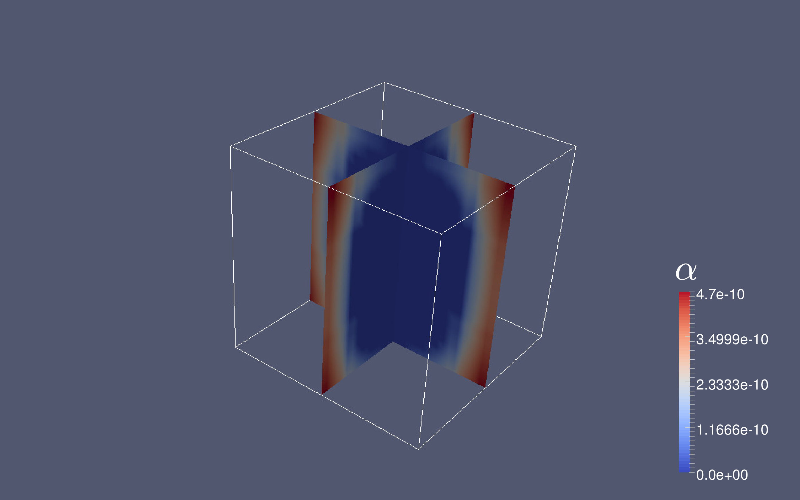 Figure 1
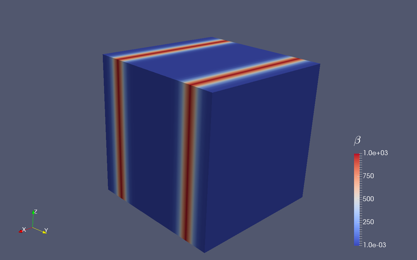 Figure 2
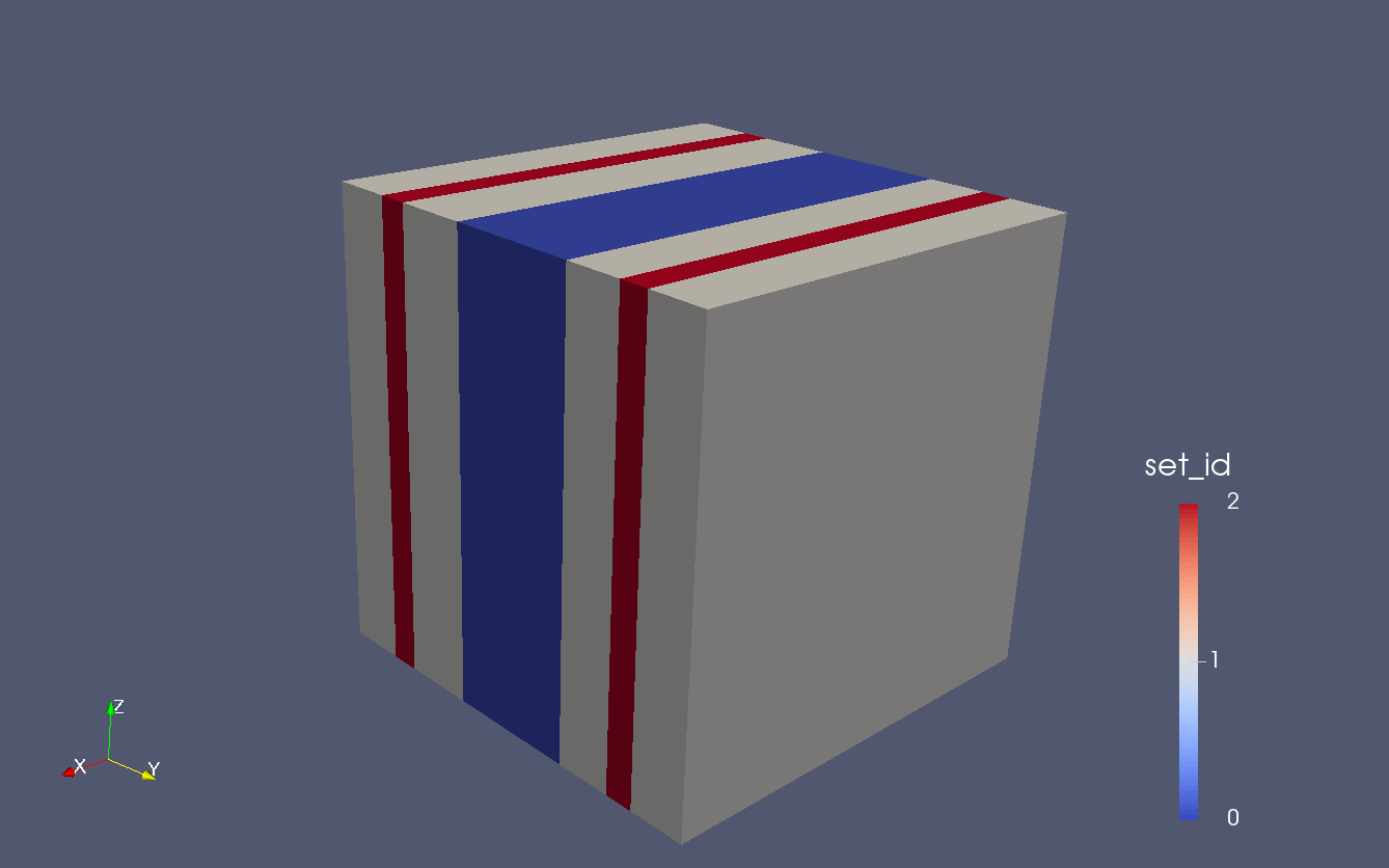 Figure 3
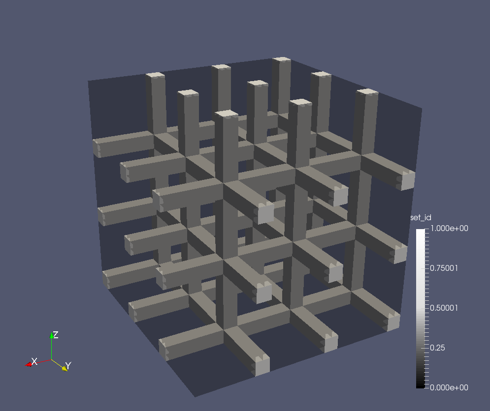 Figure 4
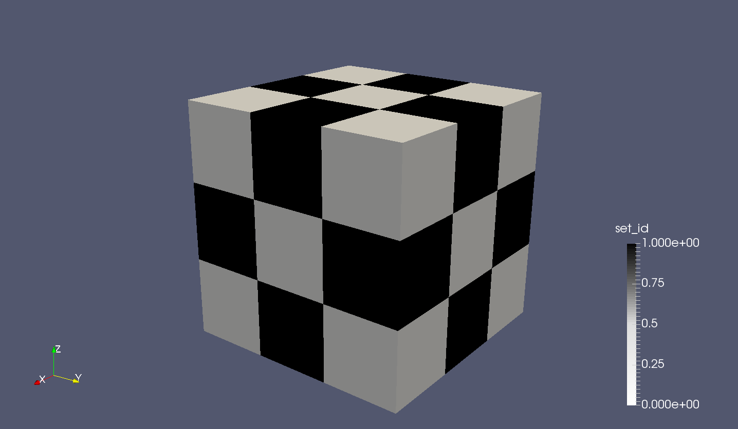 Figure 5
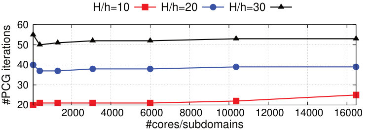 Figure 6
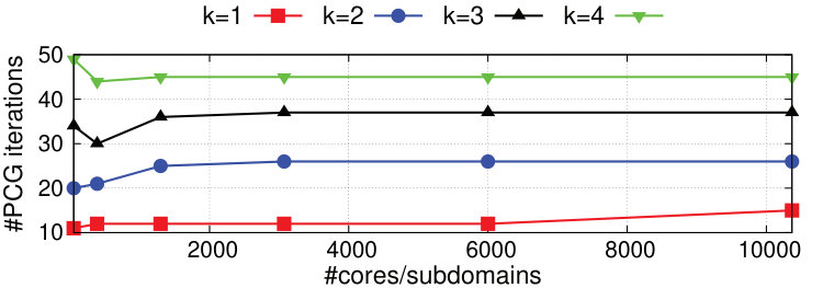 Figure 7
 Figure 8
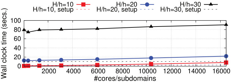 Figure 9
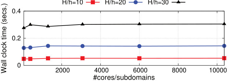 Figure 10
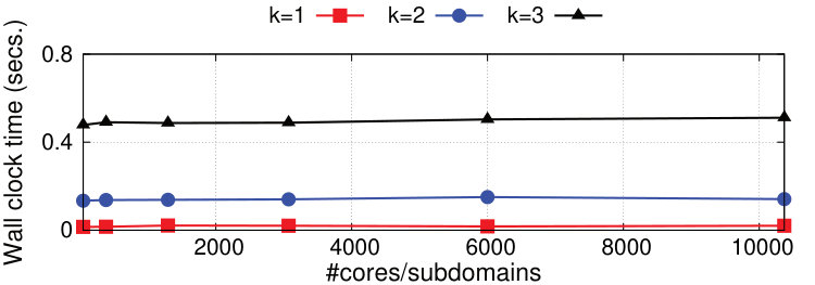 Figure 11
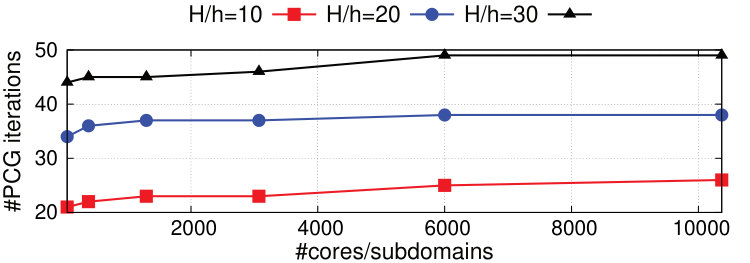 Figure 12
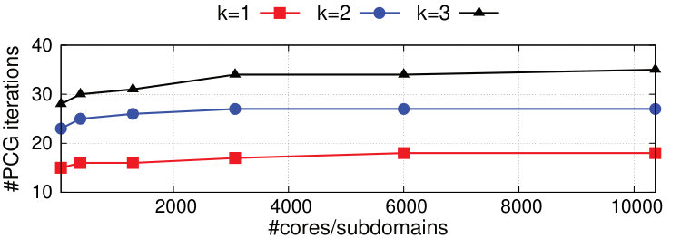 Figure 13
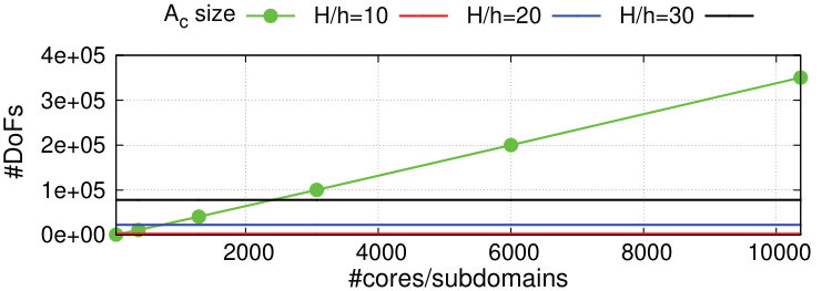 Figure 14
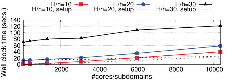 Figure 15
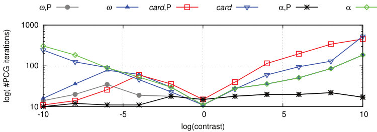 Figure 16
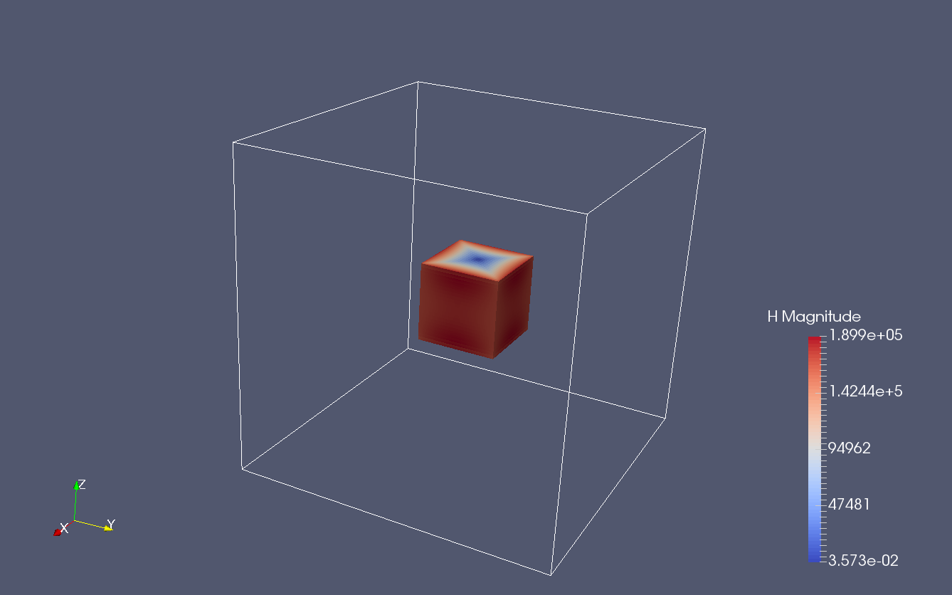 Figure 17
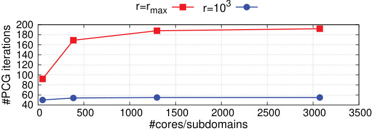 Figure 18
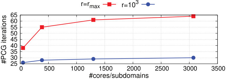 Figure 19
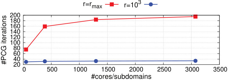 Figure 20
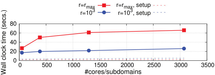 Figure 21
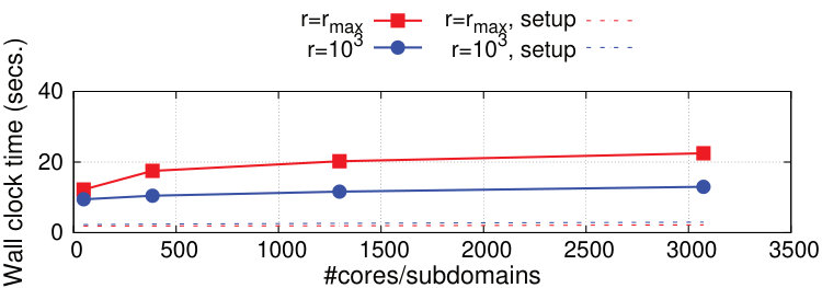 Figure 22
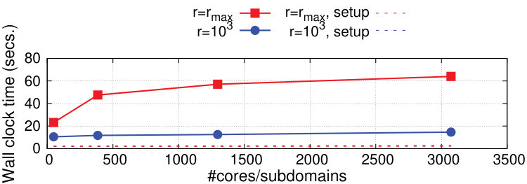 Figure 23
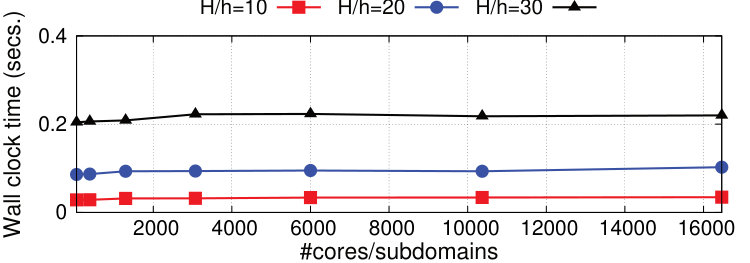 Figure 24
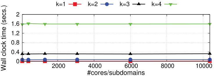 Figure 25
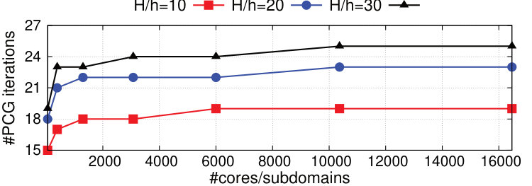 Figure 26
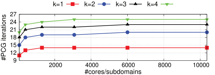 Figure 27
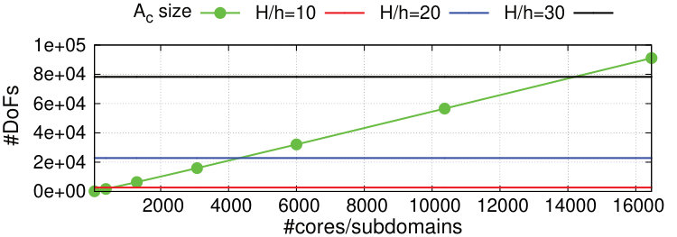 Figure 28
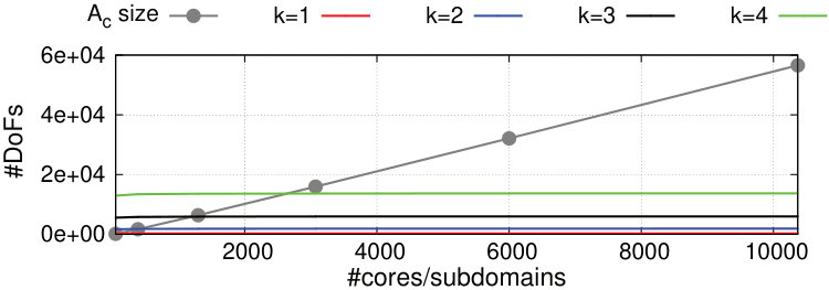 Figure 29
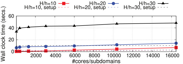 Figure 30
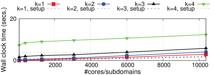 Figure 31
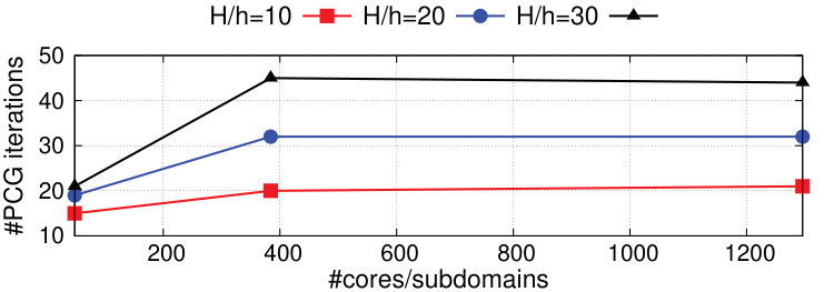 Figure 32
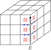 Figure 33
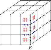 Figure 34
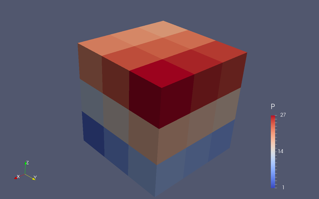 Figure 35
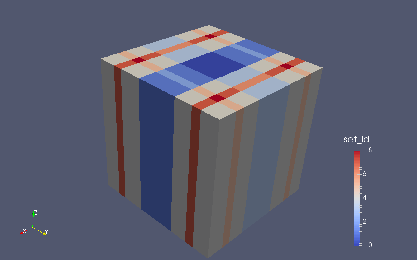 Figure 36
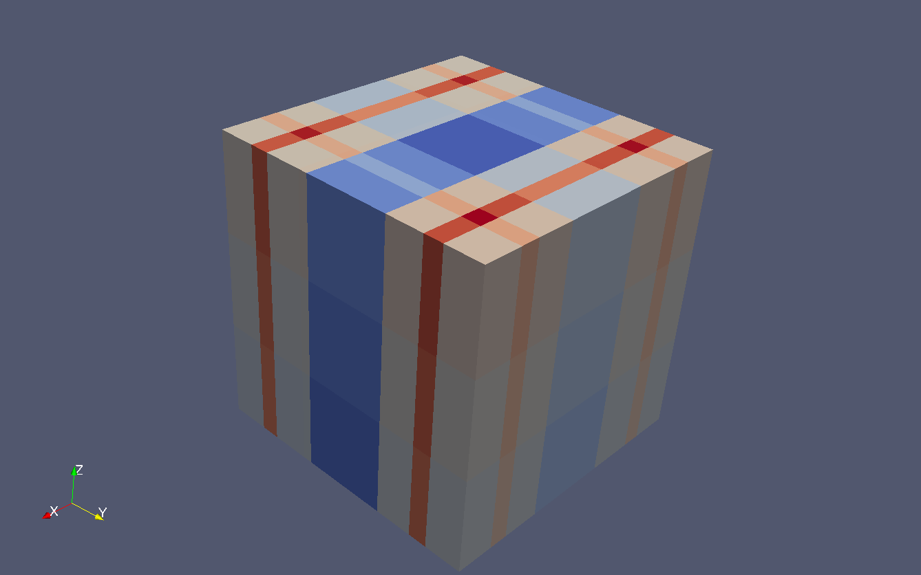 Figure 37
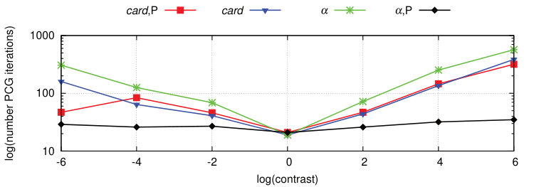 Figure 38
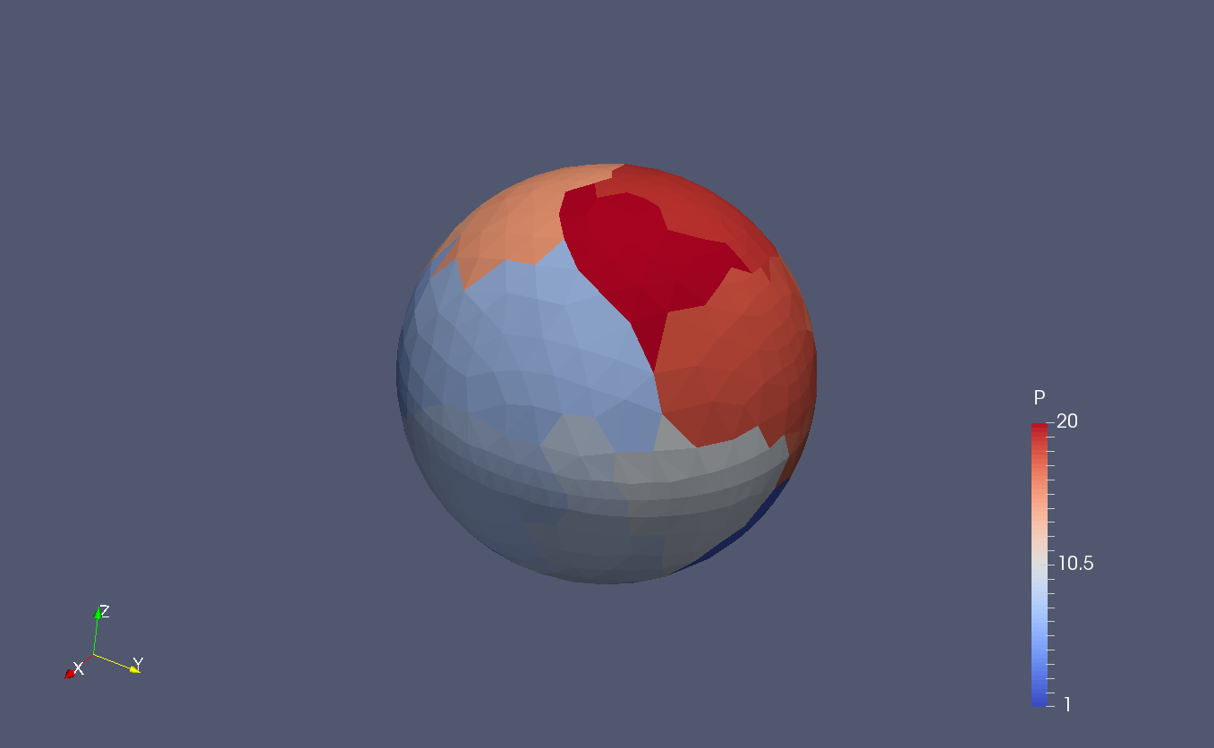 Figure 39
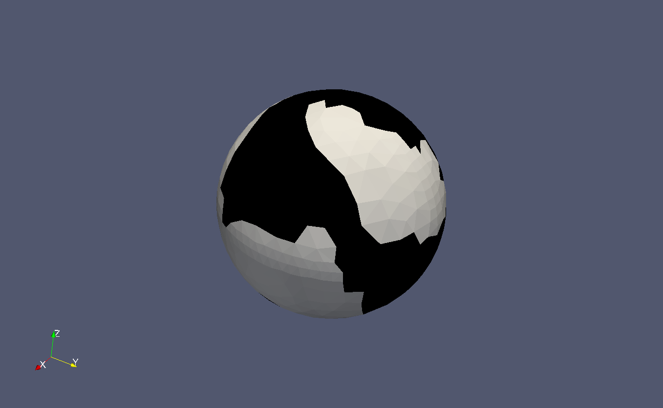 Figure 40
| / P | |||||||
| 4 | 14 | 24 | 35 | 38 | 40 | 40 | 41 |
| 8 | 26 | 37 | 61 | 65 | 70 | 69 | 70 |
| 12 | 31 | 52 | 72 | 78 | 82 | 82 | 84 |
| / P | |||||||
| 4 | 14 | 24 | 35 | 38 | 40 | 40 | 41 |
| 8 | 26 | 37 | 61 | 65 | 70 | 69 | 70 |
| 12 | 31 | 52 | 72 | 78 | 82 | 82 | 84 |
| / P | |||||||
| 4 | 8 | 9 | 10 | 10 | 11 | 12 | 12 |
| 8 | 12 | 14 | 16 | 16 | 17 | 17 | 17 |
| 12 | 15 | 22 | 21 | 21 | 21 | 21 | 21 |
| /c | 1.0 | ||||
| 4 | 36 | 29 | 13 | 31 | 74 |
| 8 | 67 | 36 | 16 | 38 | 104 |
| /c | 1.0 | ||||
| 4 | 36 | 29 | 13 | 31 | 74 |
| 8 | 67 | 36 | 16 | 38 | 104 |
| /c | 1.0 | ||||
| 4 | 14 | 14 | 11 | 13 | 14 |
| 8 | 18 | 19 | 16 | 17 | 20 |
| P | # Average iters. | Average size() | size() ratio | |
|---|---|---|---|---|
| 49 | 16.8 | 196.7 | 1.31 | |
| 385 | 18.9 | 2424.5 | 2.02 | |
| 1297 | 21.7 | 7728.7 | 1.91 |
Peer Reviews
No public reviews on file for this paper yet. If you reviewed it on a platform where reviews are public (OpenReview, ICLR, NeurIPS, ICML), you can paste yours below so the community can read it here.
Videos
No videos yet. Explain this paper in a talk, walkthrough, or lecture? Add one.
Scalable solvers for complex electromagnetics problems
Santiago Badia*†,‡*
,
Alberto F. Martín*†,‡*
and
Marc Olm*†*
Abstract.
In this work, we present scalable balancing domain decomposition by constraints methods for linear systems arising from arbitrary order edge finite element discretizations of multi-material and heterogeneous 3D problems. In order to enforce the continuity across subdomains of the method, we use a partition of the interface objects (edges and faces) into sub-objects determined by the variation of the physical coefficients of the problem. For multi-material problems, a constant coefficient condition is enough to define this sub-partition of the objects. For arbitrarily heterogeneous problems, a relaxed version of the method is defined, where we only require that the maximal contrast of the physical coefficient in each object is smaller than a predefined threshold. Besides, the addition of perturbation terms to the preconditioner is empirically shown to be effective in order to deal with the case where the two coefficients of the model problem jump simultaneously across the interface. The new method, in contrast to existing approaches for problems in curl-conforming spaces does not require spectral information whilst providing robustness with regard to coefficient jumps and heterogeneous materials. A detailed set of numerical experiments, which includes the application of the preconditioner to 3D realistic cases, shows excellent weak scalability properties of the implementation of the proposed algorithms.
Centre Internacional de Mètodes Numèrics en Enginyeria, Esteve Terrades 5, E-08860 Castelldefels, Spain. Universitat Politècnica de Catalunya, Jordi Girona1-3, Edifici C1, E-08034 Barcelona, Spain.
SB gratefully acknowledges the support received from the Catalan Government through the ICREA Acadèmia Research Program. MO gratefully acknowledges the support received from the Catalan Government through the FI-AGAUR grant. This work has been partially funded by the project MTM2014-60713-P from the “Ministerio de Economía, industria y Competitividad” of Spain. The authors thankfully acknowledge the computer resources at Marenostrum-IV and the technical support provided by the Barcelona Supercomputing Center (RES-ActivityID: FI-2018-3-0029). E-mails: [email protected] (SB), [email protected] (AM), and [email protected] (MO)
Keywords: Finite Element Method, Maxwell Equations, Domain Decomposition, Electromagnetics, Solvers.
1. Introduction
Realistic simulations in electromagnetic problems often involve multiple materials (e.g., dielectric and conducting materials), which may imply high contrasts in the coefficients describing the physical properties of the different materials. Besides, the behaviour of conducting materials may be modelled by highly variable, heterogeneous coefficients. This problem definition inevitably leads to high condition numbers for the resulting linear systems arising from curl-conforming finite element (FE) discretizations of the corresponding partial differential equation (PDE), which pose great challenges for solvers. Furthermore, the design of solvers for (curl)-conforming approximations poses additional difficulties, since the kernel of the curl operator is non-trivial. Consequently, for realistic electromagnetic simulations in 3D, the use of robust iterative solvers is imperative in terms of complexity and scalability. In this work, we will focus on the development of robust BDDC preconditioners for problems posed in (curl) involving high variation of the coefficients for the corresponding PDE.
BDDC preconditioners [1] belong to the family of non-overlapping domain decomposition (DD) methods [2]. They can be understood as an evolution of the earlier Balancing DD method [3]. These methods rely on the definition of a FE space with relaxed inter-element continuity, which is defined by choosing some quantities to be continuous across subdomain interfaces, i.e., the coarse or primal degrees of freedom. Then, the continuity of the solution at the interface between subdomains is restored with an averaging operator. The method has two properties that make it an outstanding candidate for extreme scale computing, namely it allows for aggressive coarsening and computations among the different levels can be performed in parallel. Outstanding scalability results have been achieved by an implementation in the scientific computing software FEMPAR [4, 5], which exploits these two properties in up to almost half a million cores and two million subdomains (MPI tasks) [6]. Another work showing excellent scalability properties up to two hundred thousand cores is [7], which is implemented in the software project PETSc [8].
The main purpose of this work is to construct BDDC methods for the linear systems arising from arbitrary order edge (Nédélec) FE discretizations of heterogeneous electromagnetic problems. An analysis for 3D FETI-DP111FETI-DP algorithms [9] are closely related to BDDC methods. In fact, it can be shown that the eigenvalues of the preconditioned operators associated with BDDC and FETI-DP are almost identical [10, 11, 12]. algorithms with the lowest order Nédélec elements of the first kind was given by Toselli in [13], who argued that the difficulty of iterative substructuring methods for edge element approximations mainly lies in the strong coupling between the energy of subdomain faces and edges. In short, no efficient and robust iterative substructuring strategy is possible with the standard basis of shape functions for the edge FE (see [14]). A suitable change of basis was introduced in [13] for lowest order edge elements and box-subdomains. Besides, an extension to arbitrary order edge FEs and subdomain geometrical shapes is presented in [15]. In this work, we will offer some new insights in the definition and construction of the change of basis for the latter general case. As pointed out in [16], the change of variables can be implemented in practice with just a few simple modifications to the standard BDDC algorithm [1].
Modern BDDC methods [17] propose coarse space enrichment techniques that adapt to the variation of coefficients of the problem [18, 19, 20, 21, 22, 23], where coarse DOFs are adaptively selected by solving generalized eigenvalue problems. This approach is backed up by rigorous mathematical theory and has been numerically shown to be robust for general heterogeneous problems. On the other hand, several different scalings have been proposed for the averaging operator in the literature to improve the lack of robustness of the cardinality (i.e., arithmetic mean) scaling for coefficient jumps. The stiffness222weighted averages with the diagonal entries of the operator for every DOF scaling takes more information into account but can lead to poor preconditioner performance with mildly varying coefficients [24]. A robust approach is the deluxe scaling, first introduced in [16] for 3D problems in curl-conforming spaces. It is based on the solution of local auxiliary Dirichlet problems to compute efficient averaging operators [25, 17, 26, 7, 27, 28], involving dense matrices per subdomain vertex/edge/face. However, to solve eigenvalue and auxiliary problems is expensive and extra implementation effort is required as coarse spaces in DD methods are not naturally formulated as eigenfunctions.
The main motivation of this paper is to construct robust BDDC preconditioners for problems in curl-conforming spaces that keep the simplicity of the standard BDDC method, i.e., to avoid the spectral solvers of adaptive versions, whereas keeping robustness and low computational cost. In order to do so, we follow the idea of the PB-BDDC preconditioner, presented in [29] for problems in grad-conforming spaces.
Based on the fact that BDDC methods ( and DD methods in general ) are robust with regard to jumps in the material coefficients when these jumps are aligned with the partition [2, 30], one can use a PB-partition obtained by aggregating elements of the same (or similar) coefficient value. However, using this type of partition can lead to a poor load balancing among subdomains and large interfaces. To overcome this situation, the PB-BDDC respects the original partition (well-balanced) but considers a sub-partition of every subdomain based on the physical coefficients, leading to a partition of the objects into sub-objects defined according to the variation of the coefficients. Consequently, the method is also based on an enrichment of the coarse space but with the great advantage of not requiring to solve eigenvalue or auxiliary problems, i.e., the simplicity of the original BDDC preconditioner is maintained. On the other hand, the PB-BDDC methods involve a richer interface with the application software, e.g., access to the physical properties of the problem, which is in line with the philosophy of the FEMPAR library, i.e., a tight interaction of discretization and linear solver steps to fully exploit the mathematical structure of the PDE operator. The PB-BDDC preconditioner turned out to be one order of magnitude faster than the BDDC method with deluxe scaling in [7] for linear elasticity and thermal conductivity problems with high contrast.
Our problem formulation arises from the time-domain quasi-static approximation to the Maxwell’s Equations for the magnetic field (see [31]), which involves two different operators, the mass and double curl terms. This fact certainly poses more complexities than the ones faced in [29] for the PB-BDDC solver, since it has to deal with the interplay of both (simultaneous) coefficient jumps. Our solution is to propose a simple technique to recover the scenario where only one coefficient has a jump across interfaces: we will add a perturbation at the preconditioner level so that the perturbed formulation does not involve a jump for the mass-matrix terms across interfaces. The effectiveness of the technique will be empirically shown. In order to extend the PB-BDDC algorithm to heterogeneous materials, a relaxed definition of the PB-partition will be stated where we only require that the maximal contrast of the physical coefficient in each PB-subdomain is smaller than a predefined threshold. The threshold can be chosen so that the condition number is reasonably small while the size of the coarse problem is not too large.
The article outline is as follows. The problem is defined in Sect. 2, where basic definitions are introduced. Sect. 3 is devoted to the presentation of the PB-BDDC preconditioner for heterogeneous 3D problems in (curl). In Sect. 4 we will give some implementation insights, based on our experience through the implementation of the algorithms in the scientific software project FEMPAR . In Sect. 5, we present a detailed set of numerical experiments, covering a wide range of cases and applications for the PB-BDDC preconditioner. Finally, some conclusions are drawn in Sect. 6.
2. Problem setting
Let us consider the boundary value Maxwell problem on a physical domain :
[TABLE]
where , are the resistivity and the magnetic permeability of the materials, respectively, is a unit normal to the boundary and is the 3D curl operator (see [32]). For the sake of simplicity, we consider homogeneous Dirichlet conditions, i.e., zero tangential traces on . Nevertheless, all the developments in this work can readily be applied to Neumann and/or inhomogeneous conditions, see [14] for proper definitions. In order to pose the weak form of the problem, let us define the functional space
[TABLE]
and its subspace that satisfies homogeneous Dirichlet boundary conditions,
[TABLE]
Besides, we will also make use of the space
[TABLE]
Functions in are approximated by edge FE methods of arbitrary order, which we represent by . In addition, functions in are approximated by standard scalar, continuous Lagrangian FE methods, which we represent by . The weak form of the boundary value Maxwell problem in Eq. (1) reads: find such that
[TABLE]
where
[TABLE]
2.1. Domain partition
Let us consider a bounded polyhedral domain . Let be a partition of into a set of tetrahedral or hexahedral cells . For every cell consider its set of vertices , edges , or faces . They constitute the set of geometrical entities of the cell (excluding itself) as . The union of these sets for all cells is represented with . We consider a partition of the domain into non-overlapping subdomains , obtained by aggregation of elements . These subdomains are assumed to be such that the computational cost of solving the discrete Maxwell problem in the different subdomains leads to a well-balanced distribution of computational loads among processors in memory distributed platforms. We denote by the interface of the partition , i.e., . Every subdomain can be also partitioned into the smallest set of subdomains , , such that the material properties in Eq. (1) are constant at every . For obvious reasons, we call this sub-partition a PB-partition and will be denoted by . Clearly, the resulting global is also a partition of , and there is a unique for every such that . We consider a global numbering for the PB-subdomains, i.e., , , having a one-to-one mapping between the two indices labels. Analogously, we define the interface of the PB-partition as .
2.2. Finite Element spaces
Let us define the FE spaces for every subdomain , and the corresponding Cartesian product space . Note that functions belonging to this space are allowed to have discontinuous tangent traces across the interface . The global space in which the global problem is sought, i.e., , can be understood as the subspace of functions in that have continuous tangent traces across . We can now define the subdomain FE operator , , as for all . Then, the sub-assembled operator is defined as , in which contributions between subdomains have not been assembled. The assembled operator (see Eq. (7)) is the Galerkin projection of the operator onto .
The space of edge FE functions can be represented as the range of an interpolation operator , which is well-defined for sufficiently smooth functions , by
[TABLE]
where are the evaluation of the moments, i.e., the DOF values, and are the elements of the unique basis of functions that satisfies , i.e., the shape functions. The reader is referred to [14] for a comprehensive definition of edge moments and the construction of polynomial spaces and basis of shape functions for the tetrahedral/hexahedral edge FE of arbitrary order.
2.3. Objects
In this section we introduce the definitions of global objects, or simply globs, which are heavily used in DD preconditioners (see, e.g., [2]). Given a geometrical entity and a subdomain partition , we denote by the set of subdomains in that contain . Then, we define a geometrical object as the maximal set of geometrical entities in with the same subdomain set. We denote by the set of subdomains in containing and by ndof() the total number of DOFs placed on . An object such that ndof()>0 is a face if or an edge if . In addition, an object such that ndof()=0 is a corner. Grouping together the objects of the same type, we obtain the set of corners , edges and the set of faces . Therefore, the set of globs is defined as .
Remark 2.1**.**
This definition differs from the standard one (see, e.g., [33]). It is intentionally done in order to isolate globs that do not contain DOFs, i.e., , which can be omitted in the rest of our exposition.
Once globs are defined, let us also introduce the set of PB-globs, denoted by , as classification of all into , or by considering the previous definitions based on rather than . is a sub-partition of where coefficients are subdomain-wise constant within each .
3. Physics-Based BDDC
3.1. Change of basis
Any BDDC method that employs a standard 3D edge FE basis of shape functions is bound to show a factor dependent on the element size in the condition number [13], which precludes scalability. A key aspect of the curl-conforming edge FE spaces is the fact that . One of the main ingredients of any BDDC method are the averaging operators (see detailed exposition in Sect. 3.2) that restore the continuity of the solution at the interface among subdomains. Since the averaging operators are usually based on some algebraic operations over DOF values, they are, more precisely, scaling matrices that depend on the basis being used to describe (and , by restriction to every subdomain). A key property that must hold for such operator to end up with a stable decomposition is the following: Given a function such that its local component in every processor belongs to , the restriction of the resulting function to every subdomain must belong to too. Otherwise, the energy of such functions is much increased after the averaging operation, and thus, the decomposition is not scalable. A key result in this direction is the decomposition proposed in [13] in the framework of FETI-DP methods for problems in .
Edge FE space moments can be assigned to edges/faces of the mesh (see [14]). Let us denote by the subspace of functions of such that their DOF values are not located on some or , i.e., the DOFs are interior. Clearly, . On the other hand, a function for a coarse edge admits a unique decomposition as follows (see [13, 25] for more details):
[TABLE]
with being the Lagrangian shape functions related to the internal nodes of (i.e., nodes such that ) and their cardinality, whereas . It is clear from Eq. (9) that two kinds of DOFs arise in the new basis for each subdomain edge : a DOF associated with the basis function , which represents the average tangent value over the coarse edge , and DOFs associated with gradients of scalar, Lagrangian shape functions placed at its internal nodes. An illustration for the variables in the old (original) and new basis for a given is presented in Fig. 1. Thus, we have that . As a result, admits the unique decomposition:
[TABLE]
where is the tangential vector such that , being the unit tangent to .
Let us now describe the relation between the original set of DOFs (old basis in the global space) and the one that arises from Eq. (10) (new basis) for . A function can be written in the old basis as , where is the set of global edge shape functions. Furthermore, consider the set of new basis functions , where old basis elements associated to are replaced by its corresponding functions in Eq. (9) (i.e., interior and face edge functions, Lagrangian shape functions gradients, and the coarse edge functions). The interpolation operator (see Eq. (8)) induces the change of basis matrix, whose entries are computed by evaluating the original edge moments for the introduced set of new basis functions as (Einstein notation)
[TABLE]
or in compact form, . Furthermore, we can readily define the inverse change of basis as . The usual restriction matrix is used to obtain local restrictions of the global change of basis as ; we abuse notation, using the same notation for the restriction with respect to the two bases, since it will be clear from the context. Finally, local restrictions lead to the change of basis , which will be applied for functions defined on . A detailed exposition of an implementation strategy for the change of basis is found in Sect. 4.2.
3.2. Preconditioner
Similarly to other BDDC methods, we associate coarse DOFs to some of the globs in . In particular, BDDC methods for 3D curl-conforming spaces associate two coarse DOFs to every , defined as
[TABLE]
where is an arc-length parameter, . Thus, the expression Eq. (12b) refers to the first order moment of the tangent component of the solution on the edge , in contrast to the zero-order moment in Eq. (12a). In the new basis (see Eq. (9)), it is easy to check that and [13]. Let us define the subspace as
[TABLE]
i.e., the subspace such that for all , coarse DOFs (12a) and (12b) are continuous across subdomain interfaces for all . Clearly, .
The following key ingredient in the BDDC method is the averaging operator , defined as some weighted average of the DOF values at the interface. This operator is in practice defined as a matrix for a particular choice of the basis functions for . Let us consider the new basis functions in . Given a fine edge/face , we define a weight for each as
[TABLE]
where the choice of defines the scaling: the cardinality scaling with or the -based, -based scaling with or , respectively. Besides, one can consider a weighted coefficient for , , which is also subdomain-wise constant within all in our definitions if regular structured meshes are considered. We note that all the expressions for the scalings are constant on globs by construction, due to objects generation based on with constant coefficients. Then, we define the weighted function as follows. First, we compute for every subdomain the weighted local functions as
[TABLE]
where , , and include the components related to interior, face, and edge DOFs in Eq. (10), respectively, and the corresponding weight for every interface edge/face in . Next, we sum the values of DOFs on different subdomains that represent the same DOFs in , i.e., assemble the DOFs as
[TABLE]
Next, we recover the sub-assembled bilinear form , whereas and are the Galerkin projection of onto and , respectively. We additionally define the harmonic extension operator , that, given , provides , where is a bubble function that vanishes on the interface and holds:
[TABLE]
Let us denote the Galerkin projection of onto the global bubble space by . Thus, the action of the harmonic extension operator can be written as
[TABLE]
We finally define the operator . We can now state the BDDC preconditioner as
[TABLE]
Note that having the expression of the operators associated with the new basis is essential in order to apply the averaging operator . Nevertheless, it is possible to employ the original operators in the standard basis and work with the change of basis matrix [16]. In this case, the only difference with regard to Eq. (19) is the application of the averaging operator as
[TABLE]
Application details for the change of basis are exposed in Sect. 4.2. Therefore, the definition of the preconditioner is the one of the standard BDDC [1] with a set of globs generated by a partition based on coefficients and a modification of the averaging operator to take into account this fact. Besides, one can work with the standard basis of edge FEs and use strategically the change of basis required to attain a scalable algorithm in the application of the weighting operator.
3.3. Perturbed PB-BDDC preconditioner
The presented PB-BDDC preconditioner has been shown to be robust with the jump of coefficients in the steady Poisson equation [29]. However, the problem in Eq. (1) adds the complexity of the interplay between the two different parameters and across the interface. Following the robust approach in [29], our idea is to get rid of the jump of one coefficient across the interface so the preconditioner has not to deal with the interplay between the two of them and the scenario where the method is successful is recovered. In order to decide which coefficient is affected, we consider the locality of the mass matrix operator in front of the double curl terms. The main idea is to add a perturbation in the original formulation of the preconditioner so we end up with common information for the mass matrix operator for DOFs that are replicated among different subdomains, i.e., located on the interface . Therefore, the problem posed in will only contain a jump in the double curl term across the interface.
Given a function , we can define its extension as a global function such that all DOFs belonging to are identical to the ones of and the rest are zero. The extended function has support on and its neighbours, denoted by . The perturbed preconditioner for a local subdomain is expressed as:
[TABLE]
Therefore, entries for interface DOFs in the local mass matrix will be fully-assembled instead of partially assembled, leading to common information at the interface across all subdomains. In the situation where no jump occurs for the mass matrix coefficients at the interface among subdomains, we consider the original preconditioner presented in Sect. 3.2, avoiding the perturbed formulation for obvious reasons.
Remark 3.1**.**
The definition of the original problem is not modified. We only consider the perturbed local operator in the formulation for the preconditioner.
3.4. Relaxed PB-BDDC
In previous sections, the definition of (and consequently the definition of PB-globs) is based on the requirement that coefficients are constant in each PB-subdomain, i.e., different subparts with constant coefficients can be identified in a subdomain, e.g. a problem composed by different homogeneous materials. However, physical coefficients may vary across a wide spectrum of values, even in a small spatial scale. Besides, the requirement that coefficients have to be constant in each PB-subdomain may result in an over-partitioned domain where coefficient jumps are not significant among different PB-subdomains. In order to address these situations and to deal with a more general applicability of the preconditioner, we introduce the relaxed (rPB-BDDC) extension of the preconditioner. In short, relaxed (rPB)-subdomains are not determined by constant coefficients within the original partition but we only require that the maximal contrast in each PB-subdomain is less than some predefined tolerance . We define the maximal contrast independently for each coefficient present in the problem Eq. (1), thus defining two (different) thresholds. Then, one can find a rPB-partition, which we denote by , such that
[TABLE]
where . Hence, the choice of both thresholds will determine the partition as a sub-partition of the original partition . Note that if we consider , we recover the original partition , while lower values for the thresholds lead to an increasing number of subparts, consequently globs, and thus richer coarse spaces. The rPB-BDDC preconditioner can be defined for any value of the threshold . By tuning one can obtain the right balance between computational time and robustness.
As coefficients are no longer constant in each rPB-subdomain, we propose to use averaged coefficients in Eq. (14) in order to define the averaging operator. The averaged coefficients, denoted as and , are computed in the rPB-subdomain simply as
[TABLE]
Hence, the definition of the averaging operator Eq. (14) is not modified and all DOFs on the same coarse geometrical entity are weighted by the same constant value. Thus, under the , the preconditioner expression is written exactly in the same form as in Sect. 3.2.
4. Implementation aspects
In this section, we expose implementation strategies for some key points that the authors find of interest for potential users/developers of similar methods, namely an edge partition algorithm to avoid problematic cases in (unstructured) PB-partitions, the construction of the change of basis, the implementation of the original BDDC constraints and the aggregation of cells into rPB-subdomains based on heterogeneous coefficients , and the thresholds , . For a comprehensive implementation strategy of arbitrary order curl-conforming tetrahedral/hexahedral FEs, the reader is referred to [14].
4.1. Coarse edge partition
Special care has to be taken with the general definition for subdomain edges presented in Sect. 2.3. In particular, when globs are generated based on or a partition obtained with graph partitioners, e.g. METIS, the presented definition of in Sect. 2.3 may not be sufficient for expressing the function and the coarse DOFs in the new basis. We detail the pathological cases identified in [25] (cases [1] and [2] below), and extension of a case in [25] (case [3]) plus an additional case (case [4]), for which we provide examples. We propose a unique cure, based on the partition of problematic coarse edges into coarse sub-edges such that the problematic cases are solved.
- [1]
Disconnected components. We say that fine edges are connected if they have an endpoint in common. Consequently, if a coarse edge has disconnected components, it has endpoints. Note that, while this fact does not preclude the invertibility of the change of basis, if each of the components is treated as a coarse edge we recover original meaningful definitions for continuity constraints across subdomains. 2. [2]
Interior node in touch with another subdomain. This case occurs when an internal node to does not have the same set of subdomains as , i.e., is shared by plus additional subdomains. In fact, is then an element of in the classification provided in Sect. 2.3. We recall that the change of variables is made for gradients of scalar, Lagrangian functions defined on all internal nodes of . However, if we consider a nodal shape function associated to , it will be coupled with other internal nodal DOFs for , thus introducing a coupling between an external subdomain to and itself, which is clearly not present in the original basis. A remedy for it consists of simply splitting the coarse edge into two sub-edges at the problematic node . Let us denote by the subset of this kind of nodes for all . 3. [3]
Edge -furcation. This situation occurs when a coarse edge that does not have disconnected components has more than two endpoints. At some internal node the coarse edge is -furcated into edges, so the definition of the shape function in the new basis loses its original meaning. Furthermore, this fact precludes the locality of the change of basis for every edge . In this case, a simple remedy is again to split the edge into sub-edges at any node shared by more than two edges. 4. [4]
Closed loop. In this case we cannot identify endpoints for a coarse edge and therefore define a unique orientation for it. Furthermore, the new set of basis functions is not well defined since the definition in Sect. 3.1 relies on the fact that every edge has 2 end points, thus not being applicable in this case. In this situation, an internal node for the coarse edge must be chosen as start/end point (common in all subdomains) to assign an orientation to the edge and be treated as an edge endpoint in the change of basis definition.
In order to address all the presented problematic cases we propose a simple algorithm based on a classification into sub-edges. Our goal is to find a partition of into such that every is constructed connecting fine edges that share (only) one vertex with the following edge. Therefore, every coarse sub-edge has a unique starting point, a chain of connected fine edges sharing only one node and a unique end-point, which defines its unique orientation across all subdomains. Let us consider the set of nodes , where the number of occurrences for each node is denoted by count(). First, we can identify the set of nodes where is -furcated as
[TABLE]
We note that is already identified in the glob generation algorithm. Then, we can find a partition of the set of nodes into the two following subsets:
[TABLE]
Note that by definition of interior nodes, they are such that . Such classification is performed by simply counting the number of appearances of nodes plus setting problematic nodes belonging to other objects as edge boundary nodes. Then, the coarse edge partitioning Alg. 1 finds paths from one edge boundary node (with a global criteria to select it) until the following edge boundary node. Furthermore, in this procedure we identify the direction of every fine edge with regard to its container coarse edge.
From this point onwards, we consider that each is a (sub-)edge of the original coarse edges such that they do not present problematic cases.
4.2. Change of basis
In this section we provide some implementation details of the change of basis described in Sect. 3.1. In the application of the averaging operator in Eq. (20), we note that one must apply the global change of basis and its restriction to subdomains. A practical implementation of their application in both cases can be performed with the local restriction of the change of basis to the subdomains, i.e., , thus it can be performed in parallel in distributed memory environments. The application of the inverse of the change of basis in the sub-assembled space or (Eq. (20)) can be performed in parallel, i.e., relying on the restriction of the operators to the subdomains, given its definition (see Sect. 3.1). On the other hand, the sparsity pattern of the global change of basis can be exploited in order to achieve a parallel implementation of the application of and to a function that only relies on restricted (to the subdomains) information.
Proposition 4.1**.**
The expression holds, where and .
Proof.
By definition of the change of basis matrix, it is easy to check that only depends on the DOF values of (in the new base), i.e., . Thus we can write
[TABLE]
∎
Unfortunately, this reasoning cannot be applied to the transpose of the change of basis.
Proposition 4.2**.**
Consider arbitrary local weighting diagonal matrices for every subdomain such that , i.e., they form a partition of the unity. Then, the expression holds, where and .
Proof.
Using the fact that is the identity matrix and the fact that (as above), it holds:
[TABLE]
∎
Therefore, the application of the change of basis can rely only on restrictions of the same to subdomains whereas the application of the transpose change of basis can be performed in parallel with subdomain restrictions plus nearest neighbour communications. With this purpose in mind, we detail here how to implement the restriction of the change of basis local to subdomains. Let us define a partition of the DOFs in into three subsets of DOFs, namely: the DOFs placed on , the DOFs placed on interface edges/faces such that , and the remaining DOFs in , denoted by , and , respectively. Furthermore, let us consider that DOFs in are sorted such that DOFs belonging to the same coarse edge are found in consecutive positions. Note that shape functions associated to , are common in both (i.e., old and new) bases. For edge FEs of order , moments (i.e., DOFs) are defined on each . Let us denote by the number of fine edges . Then, the total number of DOFs on a coarse edge is . On the other hand, the number of Lagrangian-like DOFs interior to (i.e., excluding ) is , i.e., the number of shape functions of the type . The change of basis is completed with the addition of the function to the new basis so that the dimension of both bases coincides. For the sake of illustration, both sets of basis functions restricted to are depicted in Fig. 1.
Let us denote by the number of coarse edges for a given subdomain. Then, we define the change of basis , local to every as
[TABLE]
where , , are the (original basis) edge moments defined on (the superscript in has been introduced to show that it depends on the coarse edge). We can now define the change of basis local to coarse edges. We remark that the same orientation for every coarse edge must be defined on the set of subdomains . Otherwise, the definition of the new basis function is not consistent across subdomains. In addition, the change of basis must take into account the effect of the new DOF values associated to and for in the old values . Thus, we evaluate for all indices of shape functions associated to
[TABLE]
where corresponds to the index of all moments associated to . We recall that, by definition, . The application of the moments to the (original) shape functions associated to results in . Finally, DOFs in are invariant under the change of basis. Note that the definition of Eqs. (28) and (29) related to the gradients of the scalar shape functions coincides with the so-called discrete gradient operator related to these functions, as used in [15]. However, we prefer to motivate the change of basis with the usage of the Nédélec interpolator, since it naturally provides the definition of the entries related to the unit tangent function, while suitable eigenvectors to complete the change of basis are computed in [15]. The structure of the change of basis restricted to a subdomain is
[TABLE]
where it becomes clear the fact that the inverse of the change of basis is well defined if and only if is invertible. In turn, will be invertible if and only if every change of basis local to (Eq. (28)) is invertible.
Remark 4.3**.**
Although it is used in this exposition for the sake of clarity, we do not require any particular ordering of DOFs in a practical implementation of .
4.3. BDDC constraints
In this subsection we propose a practical manner of computing the BDDC constraints Eqs. (12a) and (12b) for local problems. In our implementation, constraints over local problems are strongly imposed through the usage of Lagrange multipliers on the original basis. Therefore, the local matrix is extended with the discrete version of the constraints in order to obtain constrained (Neumann) local problems.
The computation of constraints requires to integrate zero and first order moments for the solution over all coarse edges . We note that the first constraint Eq. (12a) can be easily implemented for -order edge FEs as
[TABLE]
where we used the partition of the scalar, unit function into the set of Lagrangian test functions belonging to the polynomial space of order . These functions are used for defining the local moments on every as , (see [14] for details). Its duality with basis shape functions, i.e., , has been used in Eq. (31). Thus, to compute the first constraint one only needs to add at the corresponding entry in for each DOF, where the sign is determined by the agreement between fine and coarse edge orientations, i.e., . On the other hand, the computation of the second constraint Eq. (12b) requires to define an arc-length parameter over . A practical implementation of the constraint Eq. (12b) can avoid it by considering the constraint in the new basis. Since vanish at , integration by parts yields [13]
[TABLE]
where the contribution of is null due to the antisymmetry of the product ( we recall that ) over . Then, we can apply the change of basis to obtain the expression in the original basis, i.e., .
4.4. Building
In the rPB-BDDC method, a partition is used such that the maximal contrast, for each one of the coefficients, is lower than a predefined tolerance in each subdomain. Our goal is to identify a partition of every subdomain into subdomains where the thresholds and are respected. It can be accomplished using different algorithms. One approach is to consider a seed cell and aggregate the surrounding cells such that the contrast(s) are below the given threshold(s), proceeding recursively until no neighbouring cells can be aggregated. We take another seed among the non-aggregated cells and proceed again until all cells have been processed.
Alternatively, one can first determine the maximum and minimum values for and in a given subdomain . With this information and the thresholds , , we can determine the number of sub-intervals for every subdomain and coefficient as follows. First, we compute and as the smallest positive integers for which
[TABLE]
respectively. One can now define the intervals
[TABLE]
for , . Cells with their coefficients on the same interval are aggregated in a PB-subdomain. Those cells that have coefficients across multiple sub-intervals are treated as additional PB-subdomains. This definition allows one to isolate cells that contain abrupt jumps in the value of the coefficients, while the user has the freedom to select the thresholds such that unnecessary extra PB-subdomains are avoided.
For the sake of illustration, we include an example where all the different subset indices are presented for a unit cube domain: the original partition into subdomains in Fig. 2(a), the aggregation of cells into subsets based on (see Fig. 3(a)) for in Fig. 3(b), combined with an analogous partition for leading to a coefficient-based partition in Fig. 2(b) and the final rPB-partition in Fig. 2(c).
We note that the preconditioner is very robust despite the presence of subdomains with large aspect ratios. Support to this observation can be found in [29] (see Remark 3.12 and the corresponding numerical experiments).
5. Numerical results
In this section we evaluate the weak scalability of the proposed preconditioner for the problem in Eq. (1), within the preconditioned conjugate gradient (CG) Krylov iterative solver. The robustness of the rPB-BDDC-CG solver is tested in 3D simple domains, which are discretized either with structured or unstructured meshes. As performance metrics, we focus on the number of rPB-BDDC preconditioned CG iterations required to attain the convergence criteria, which is defined as the reduction of the initial residual algebraic -norm by a factor . On the other hand, the total computation time will be presented, which will include both preconditioner set-up and the preconditioned iterative solution of the linear system in all the experiments reported. The particular definition of coefficients and and its distribution will be specified throughout the section for each case.
We have also applied a plain CG solver for the different tests, but the results of the latter are not reported here due to its poor performance. As an example, for the same problem set-up as in Fig. 8, only 48 processors, and , it did not satisfy the convergence criteria within a prescribed maximum of 20,000 iterations, for which it consumed 144 secs, far beyond the proposed rPB-BDDC preconditioner.
5.1. Experimental framework
The rPB-BDDC methods have been implemented in the scientific software project FEMPAR [4]. FEMPAR , developed by the Large Scale Scientific Computing (LSSC) team at CIMNE-UPC, is a parallel hybrid OpenMP/MPI, software package for the massively parallel FE simulation of multiphysics problems governed by PDEs. FEMPAR offers a set of flexible data structures and algorithms for each step in the simulation pipeline, which can be customized in order to meet particular application problem needs. See [5] for a thorough coverage of the software architecture of FEMPAR . Among other features, it provides the basic tools for the efficient parallel distributed-memory implementation of substructuring DD solvers [33, 6], based on a fully-distributed implementation of data structures involved in the parallel simulation. The parallel codes in FEMPAR heavily use standard computational kernels provided by BLAS and LAPACK. Besides, through proper interfaces to several third party libraries, the local constrained Neumann problems and the global coarse-grid problem can be solved via sparse direct solvers. FEMPAR is released under the GNU GPL v3 license, and is more than 300K lines of Fortran200X code long following object-oriented design principles. In this work, we use the overlapped BDDC implementation proposed in [34], with excellent scalability properties. It is based on the overlapped computation of coarse and fine duties. As long as coarse duties can be fully overlapped with fine duties, perfect weak scalability can be attained. We refer to [6] for more details.
The experiments in this section have been performed on the MareNostrum-IV [35] (MN-IV) supercomputer, hosted by the Barcelona Supercomputing Center (BSC). In all cases, we consider a one-to-one mapping among subdomains, cores and MPI tasks. Provided that the algorithm allows for a high degree of overlapping between fine and coarse duties, an additional MPI task is spawn into a full node (i.e., 48 cores) in order to perform the coarse problem related tasks. The multi-threaded PARDISO solver in Intel MKL is used to solve the coarse-grid problem within its computing node.
Unless otherwise stated, the problem Eq. (1) will be solved in the unit cubic domain with Dirichlet homogeneous boundary conditions on the whole boundary and the forcing term . Let us denote by the usual mesh element size, and by the size of the subdomain. Then, local problem sizes can be characterized in a structured mesh and partition by . In order to perform a weak scalability analysis, we build a set of structured meshes consisting on hexahedra. A uniform partition of the meshes into subdomains is considered, where local problem sizes are .
5.2. Homogeneous problem
Let us first consider homogeneous coefficients for the whole domain . We test the problem with different local problem sizes and FE orders. In this case, the PB-BDDC preconditioner reduces to the standard BDDC preconditioner since . In Fig. 4, we present weak scalability results for the homogeneous problem up to 16464 subdomains with different local problem sizes , where the largest case has more than DOFs. We present the number of solver iterations until convergence in Fig. 4(a), and employed wall clock times in Fig. 4(b), which are composed by the preconditioner set-up time and the solution time with the BDDC preconditioned solver. The plots indicate that both the algorithm and its implementation in FEMPAR have excellent weak scalability properties. Provided that the algorithm overlaps fine and coarse tasks, coarse tasks computing times are masked as long as they not exceed computing times for local problems, which allow us to observe excellent weak scalability times for the largest case in Fig. 4(b). The size of both local and coarse problems is presented in Fig. 4(c). Finally, we add a plot (Fig. 4(d)) of the time needed to set-up the change of basis, which includes the edge partition algorithm (Alg. 1) to detect problematic cases, to show that consumed time is only dependent on the local problem size and not significant compared to the one spent in the solver run.
Fig. 5 shows the weak scalability results for an homogeneous problem with constant coefficients and different FE orders up to 4. First, the number of iterations is (asymptotically) constant, thus the method is scalable. In this case, local problem sizes are such that the coarse problem is larger from an small number of subdomains (see Fig. 5(c)), thus it is reflected in the solver times plot in Fig. 5(b). In Fig. 5(d), the time spent in the set-up of the change of basis is presented. Out of the presented results for the homogeneous case, a clear conclusion can be drawn for the standard BDDC: the algorithm and its implementation have excellent weak scalability properties.
5.3. Multi-material problem
5.3.1. Checkerboard distribution
The checkerboard arrangement of coefficients is a widely used distribution of materials to test the robustness of the BDDC algorithms for problems in (curl) against the jump of coefficients across the interface [13, 25]. In short, it is a bi-material distribution of subdomain-wise constant coefficients such that every subdomain presents a jump of coefficients through the faces to all its neighbours. For the sake of ease, let us distinguish between black and white subdomain materials, see Fig. 6(a). Note that in the checkerboard distribution case, the jumps of coefficients are aligned with the partition, thus .
We first test the robustness of the algorithm against the contrast of the coefficients. Consider a partition of a unit cube domain with a checkerboard distribution of coefficients such that and , . The contrast is defined here as . With the variation of the value for in the range we test all the possible scenarios, namely the mass dominated problem and the curl dominated problem . The number of iterations with the contrast of the coefficients for different configurations of the preconditioner is presented in Fig. 7. Out of the plot, the most salient property is the robustness of the perturbed preconditioner (see Sect. 3.3) with the contrast of the coefficients. In fact, the original formulation of the preconditioner suffers from a large number of iterations when the contrast between the two coefficients is large, specially in the curl-dominated case. Therefore, the proposed perturbation of the preconditioner is essential to achieve a robust preconditioner, in the case where both coefficients and jump across the interface. Clearly, the perturbed formulation only has a (negligible) negative impact in the case , since actually no jump occurs across the interface. In the curl-dominated limit, and -based scalings show the same behaviour, as it is suggested by the definition of when . On the other hand, when the coefficient becomes dominant, the choice of cardinal and -based scalings also leads to good scalability results in the limit. In summary, the combination of the perturbed formulation and -based scaling is the most robust approach. Unless otherwise stated, this combination will be used throughout the section.
Let us now consider a checkerboard arrangement of coefficients such that , and and . In order to show the importance of the perturbed formulation of the preconditioner for jumps of both coefficients across interfaces, we collect the number of iterations for the original and perturbed preconditioner in Tabs. 1(a) and 1(b), respectively. The problem is solved with a partition of the unit cube and the -based scaling is employed in both cases. Iteration counts for the perturbed preconditioner are noticeably lower in all cases without exception.
Once we have shown the importance of the perturbed formulation, we present a weak scalability analysis up to 16,464 subdomains and the checkerboard arrangement of materials with the perturbed preconditioner. Problem sizes in this experiment coincide to the ones presented for the homogeneous problem in Fig. 4(c). As expected, plots in Fig. 8 show excellent scalability properties of the preconditioner in this case, i.e., the preconditioner is robust with jumps of coefficients across the interface. Although higher values of lead to a significantly higher number or iterations, these ones are (asymptotically) constant and remain in a reasonable range, see Fig. 8(a). On the other hand, Fig. 9(a) presents the number of iterations for different order FEs and problem size , which also is shown to be scalable. Out of the contrast and scalability results, we would like to remark the following issues. First, the perturbed formulation of the preconditioner is essential to achieve a robust preconditioner. Second, the method is weakly scalable for problems with high coefficient jumps across interfaces for different local sizes and FE orders.
In order to show the robustness of the method not only with structured, regular hexahedral meshes we solve the problem for a spherical domain and partition with a graph partitioner METIS. Let us consider a spherical domain with , discretized with an unstructured tetrahedral mesh containing around 50,000 cells. In order to achieve high contrast of coefficients across interfaces, a bi-material distribution of coefficients is assigned such white or black subdomain-wise constant materials are randomly assigned, see Fig. 10(b) for an illustration. The definition of the sets of coefficients is , and and . Fig. 11 shows the number of iterations with the original and the perturbed formulation of the preconditioner. The perturbed preconditioner, combined with a -based scaling, is the unique method shown to be robust with regard to the coefficients contrast, reproducing the behaviour observed in the structured case.
5.3.2. Multiple channels
In this arrangement of materials we have a background domain, denoted by black region, and a set of inclusions, denoted by white regions, that cross the domain from one boundary to the opposite one in parallel to the axes directions. We include one channel per direction per subdomain so that with an increasing number of subdomains we are solving a harder problem with channels. Channels are parallel to the axes and are positioned in the lowest (i.e, minimum coordinates) corners within every subdomain. They have a squared cross-section of size , thus occupying a volume in every subdomain, see Fig. 6(b) for an illustration of a partition of the unit cube with the described channel inclusions. The distribution of coefficients is such that contains coefficient jumps within each subdomain and also across all interfaces, thus the perturbed formulation of the PB-BDDC preconditioner will be employed.
Let us first compare the number of iterations for the PB-BDDC preconditioner against the ones that one would have with the standard BDDC, where the definition of globs is generated with the original partition . In Sect. 5.3.1, the effectiveness of the perturbation formulation has been empirically shown. Consequently, in order to provide a fair comparison among them, the perturbed formulation is considered for both preconditioners. On the other hand, while -based scaling is shown to be the most robust approach for PB-BDDC preconditioner, it miserably fails when considered with the standard globs, i.e., given by . In this case, a better result is obtained with cardinality scaling. Tabs. 2(a) and 2(b) show iteration counts for the described BDDC and PB-BDDC preconditioners, respectively, for the solution of the channels problem with and a partition of the unit cube into subdomains with local size . We define the coefficients , while we distinguish between and , which allow us to define the contrast as . As expected, the PB-BDDC preconditioner is robust with the contrast of coefficients. On the other hand, the number of iterations increases for the BDDC preconditioner in the curl-dominated case.
The following experiment evaluates the weak scalability properties for a channel-type distribution of materials. In Figs. 12 and 13 we present weak scalability results for different problem sizes and FE orders. The most salient property out of these plots is that the number of iterations is asymptotically constant for all cases. However, coarse problem sizes become larger as the partition into PB-subdomains generates a higher number of coarse DOFs, see Fig. 12(c). In this context, the coarse problem is larger than local problem sizes from an small number of subdomains, thus coarse tasks will predominate computing times precluding wall clock time scalability, as it is shown in Fig. 12(b). In Figs. 12(d) and 13(b) we present scalable wall clock times for the change of basis set-up, for different local problem sizes and FE orders.
We would like to remark that the proposed PB-BDDC preconditioner is weakly scalable for the number of iterations until convergence not only with regard to the jump of coefficients across interfaces but also for distributions of different materials within each subdomain. A multilevel version of the preconditioner for curl-conforming spaces [15], not addressed in this work, is expected to push forward the limits of the computing times scalability results.
5.4. Heterogeneous problems
In this section we study the scalability of the rPB-BDDC method for problems where the coefficients are described by continuous (at least element-wise) functions, which contain high contrasts for their maximum and minimum values. In order to build the rPB-partition, the approach based on the aggregation of cells with their coefficients on the same interval Eq. (34) is used, see Sect. 4.4.
5.4.1. Periodic analytical functions
In this case, and are defined as exponential functions with a sinusoidal exponent such that the function is periodic on the domain and the number of peaks scales with the number of original subdomains in , thus solving a harder problem as we increase the number of processors. In particular, let us consider and , where denotes the number of subdomains per () direction in a structured partition, (see depicted in Fig. 3(a) for the case , ). Clearly, the maximum contrast within each coefficient is given by . We present weak scalability results up to 3072 subdomains for two different thresholds , and for a local problem size of in three different scenarios: coefficients (Fig. 14), (Fig. 15) or both are heterogeneous (Fig. 16), being set to , otherwise. Out of these plots, we can draw some conclusions. First, the case where only is heterogeneous converges in a lower number of iterations compared to problems with heterogeneous . Secondly, the consideration of lower values for consequently results in larger coarse problems, but its size is only (approximately) doubled when only one coefficient is heterogeneous or (approximately) quadrupled when both are defined heterogeneous. In fact, in the range of subdomains considered in this experiment, the coarse problem computational times in all cases can be masked by local problem ones (Figs. 14(b), 15(b) and 16(b)). Finally, and most salient, the rPB-BDDC method with is weakly scalable in all cases with an excellent reduction in the number of iterations and computing times compared to the case where .
5.4.2. High Temperature Superconductors
Next, we study the scalability of the algorithm with a practical application, the modelling of High Temperature Superconductors (HTS). The problem consists in the magnetization of a superconducting cube completely surrounded by a dielectric material (see Fig. 18(a)), subjected to an external AC magnetic field. The formulation Eq. (1) arises in the time-domain quasi-static approximation of the Maxwell’s equations for solving the magnetic field, see [31] for details. Furthermore, the standard Backward Euler method is used to perform time integration over a time interval , so let us define a time partition into time elements. Then, the form Eq. (1) can be used to compute the magnetic field for a particular time , provided the solution on the previous time . The coefficient is affected by the current time step size as , where is the magnetic permeability of the vacuum. While the dielectric material is modelled with a constant value for , the superconducting material behaviour is modelled with the stiff nonlinear dependence of the resistivity with the solution as , with , and . The equivalence with Eq. (1) is completed by considering the source term and the strong imposition of an external magnetic field over the whole boundary. For the time step , the weak form of the nonlinear problem reads: find such that
[TABLE]
In order to derive the linearized form with Newton’s method we consider the current approximation and a (small) correction for the iterate such that . We plug the expression in Eq. (35), consider a first order Taylor expansion of around and neglect the quadratic terms with respect to , which yields the linearized problem: find such that
[TABLE]
where
[TABLE]
Therefore, the rPB-BDDC preconditioner is applied to the linearized problem Eq. (36) at every nonlinear iteration of every time step. We will focus on the performance of the linear solver, and the reader is directed to [31] for a detailed exposition of the composition of the used transient nonlinear solver.
The problem is solved in , composed by an outer dielectric material which includes a concentric superconducting cube of size 10 mm such that , see Fig. 18(a). There is no source term and Dirichlet-type boundary conditions are imposed over the entire boundary as the time-dependent magnetic field , where and . We solve the problem in the time interval , which corresponds to a quarter of a full cycle in the applied . Initial conditions are simply . The partition is obtained in all simulations for . The nonlinear scheme is stopped when the -norm of the nonlinear residual (Eq. (37b)) is below , while the convergence criteria for the rPB-BDDC preconditioned linear solver is the reduction of the initial -norm of the residual of the linearized system by .
We first present weak scalability results for the first set-up and solve with the rPB-BDDC preconditioner in Fig. 17, i.e., the first linearized problem (Eq. (36)) for the first time step. We include results for . As expected, the method shows good weak scalability properties in number of iterations (see Fig. 17(a)) and computing times (see Fig. 17(b)).
Next, we present average counters for the total number of linear solver applications for the simulation of the whole time interval ms in Table 3, for a local problem size of and different partitions. The resulting aggregation of cells into subsets based on their physical coefficient (see Sect. 4.4) for ms is depicted in Fig. 18(c). We can identify two main regions in the distribution of (see Fig. 18(b)): an inner region that is still not magnetized (i.e., with null resistivity) and a surrounding region, separated by a thin layer. Therefore, the selected value for allows us to capture the behaviour of the different regions in . Out of the results in Tab. 3, the most salient property is the (asymptotic) scalability in the average number of iterations. Besides, we show how the coarse problem size for the presented cases is only (approximately) doubled regarding to the size that would be obtained with the partition instead of the .
6. Conclusions
In this work, we have proposed an extension of the BDDC preconditioners for arbitrary order curl-conforming spaces that are robust for heterogeneous problems with high contrast of coefficients. The main idea is to enrich the continuity constraints enforced among subdomains (i.e., coarse DOFs) for those which contain high contrast of coefficients. The approach, which is shown to be robust for the grad-conforming case in [29], makes use of the knowledge about the physical coefficients to define a sub-partition of the original edge FE-based definition of coarse objects (edges and faces). The motivation for that is the well-known robustness of DD methods when there are only jumps of physical coefficients across the interface between subdomains. However, our case is more complex than the one in [29] for Poisson and elasticity problems, since two different coefficients are involved in the time-domain quasi-static approximation to the Maxwell’s equations. Our solution is to add a perturbation term to the preconditioner so as we recover a scenario similar to the one in which only one coefficient jumps across the interface. A relaxed definition of the PB subdomains, where we only require that the maximal contrast of the two physical coefficients is smaller than a predefined thresholds, allows one to extend the range of applicability of the preconditioner to truly heterogeneous materials. Our preconditioners, which use the crucial change of variables in [13] to obtain weakly scalable algorithms for problems in (curl) with few modifications to the standard BDDC algorithm in [1], are empirically shown to be robust with the contrast of coefficients. We would like to remark that our preconditioners maintain the simplicity of the standard BDDC and do not require to solve any eigenvalue or auxiliary problem.
We devoted a section to describe all the non-trivial implementation issues behind the method based on our experience through the implementation of the preconditioners in FEMPAR . Its task-overlapping implementation of the PB-BDDC preconditioner allows one to mask the computing times for the coarse problem, as long as they do not exceed local solvers time. With such implementation, we have been able to provide notable weak scalability results in the application of our new preconditioners to a wide range of multi-material and heterogeneous electromagnetics problems, including realistic 3D problems where coefficients can be defined by arbitrary functions, even dependent on the solution itself. In the future, the multilevel extension of the algorithm is expected to push forward the limits of its scalability properties.
The reference list from the paper itself. Each links out to its DOI / PubMed record.
- 1[1] C. R. Dohrmann. A preconditioner for substructuring based on constrained energy minimization. SIAM Journal on Scientific Computing , 25(1):246–258, 2003.
- 2[2] A. Toselli and O. Widlund. Domain Decomposition Methods: Algorithms and Theory . Springer-Verlag, Berlin, 2005.
- 3[3] J. Mandel. Balancing domain decomposition. Communications in Numerical Methods in Engineering , 9(3):233–241, 1993.
- 4[4] S. Badia, A. Martín, and J. Principe. FEMPAR Web page. http://www.fempar.org , 2018.
- 5[5] S. Badia, A. F. Martín, and J. Principe. FEMPAR : An object-oriented parallel finite element framework. Archives of Computational Methods in Engineering , 25(2):195–271, 2018.
- 6[6] S. Badia, A. F. Martín, and J. Principe. Multilevel balancing domain decomposition at extreme scales. SIAM Journal on Scientific Computing , pages C 22–C 52, 2016.
- 7[7] S. Zampini. PCBDDC: A class of robust dual-primal methods in PET Sc. SIAM J. Sci. Comput. , 38:S 282–S 306, 2016.
- 8[8] S. Balay, S. Abhyankar, M. F. Adams, J. Brown, P. Brune, K. Buschelman, L. Dalcin, V. Eijkhout, W. D. Gropp, D. Kaushik, M. G. Knepley, D. A. May, L. C. Mc Innes, K. Rupp, B. F. Smith, S. Zampini, H. Zhang, and H. Zhang. PET Sc Web page. http://www.mcs.anl.gov/petsc , 2018.