On a Class of Singularly Perturbed Elliptic Systems with Asymptotic Phase Segregation
Farid Bozorgnia, Martin Burger

TL;DR
This paper investigates singularly perturbed elliptic systems modeling phase segregation, proving existence, uniqueness, and asymptotic convergence to a free boundary problem with novel explicit solutions and numerical simulations.
Contribution
It introduces a new method for solving the limiting free boundary problem explicitly for specific parameters, advancing understanding of phase segregation models.
Findings
Proved existence and uniqueness of solutions.
Established convergence to a free boundary limit.
Provided explicit solutions and numerical simulations.
Abstract
This work is devoted to study of a class of elliptic singular perturbed systems and their singular limit to a phase segregating system. We prove existence and uniqueness and study the asymptotic behaviour with convergence to a limiting problem as the interaction rate tends to infinity. The limiting problem is a free boundary problem such that at each point in the domain at least one of the components is zero which implies simultaneously all components can not coexist. We present a novel method, which provides an explicit solution of limiting problem for special choice of parameters. Moreover, we present some numerical simulations of the asymptotic problem.
Click any figure to enlarge with its caption.
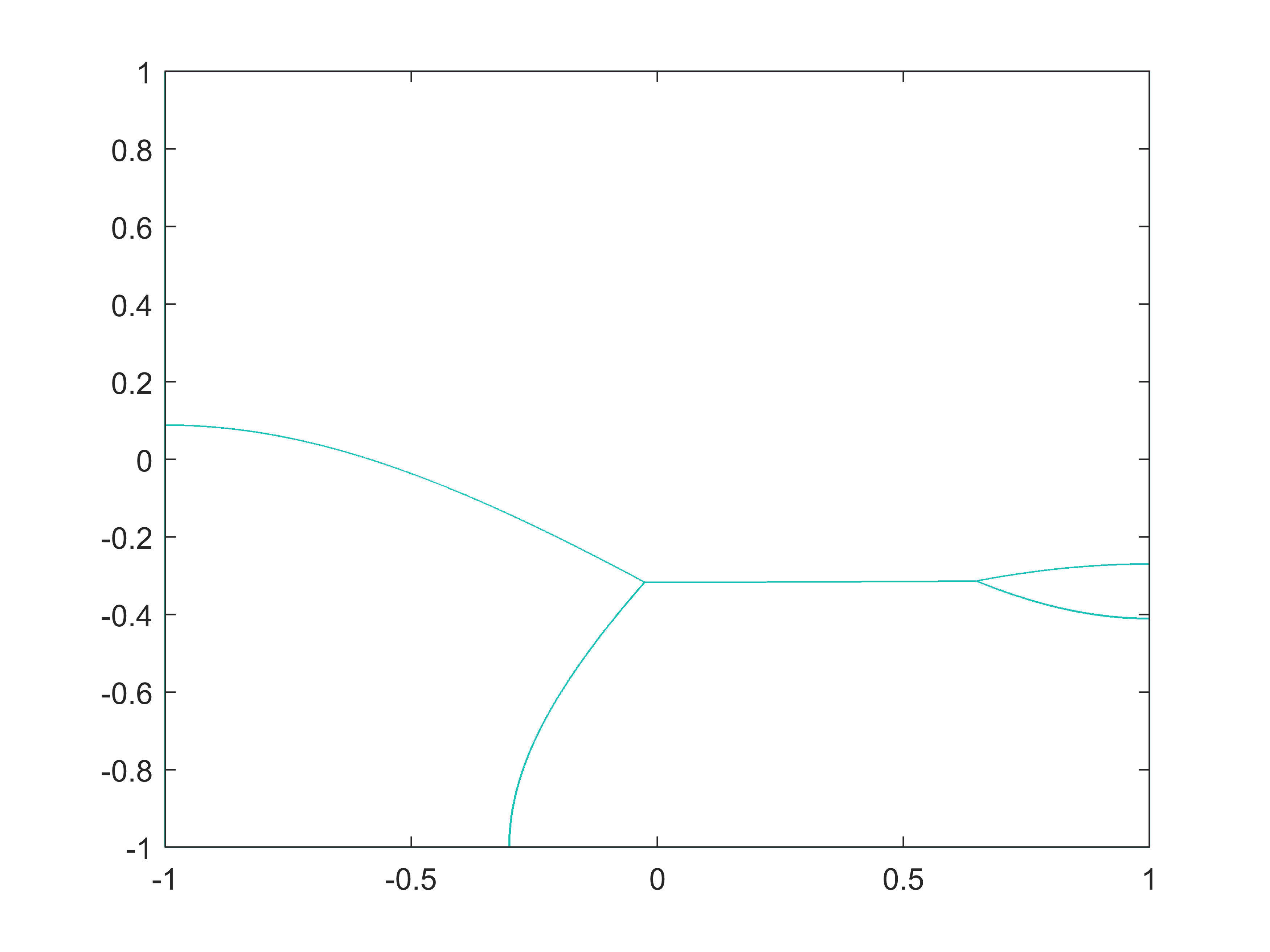 Figure 1
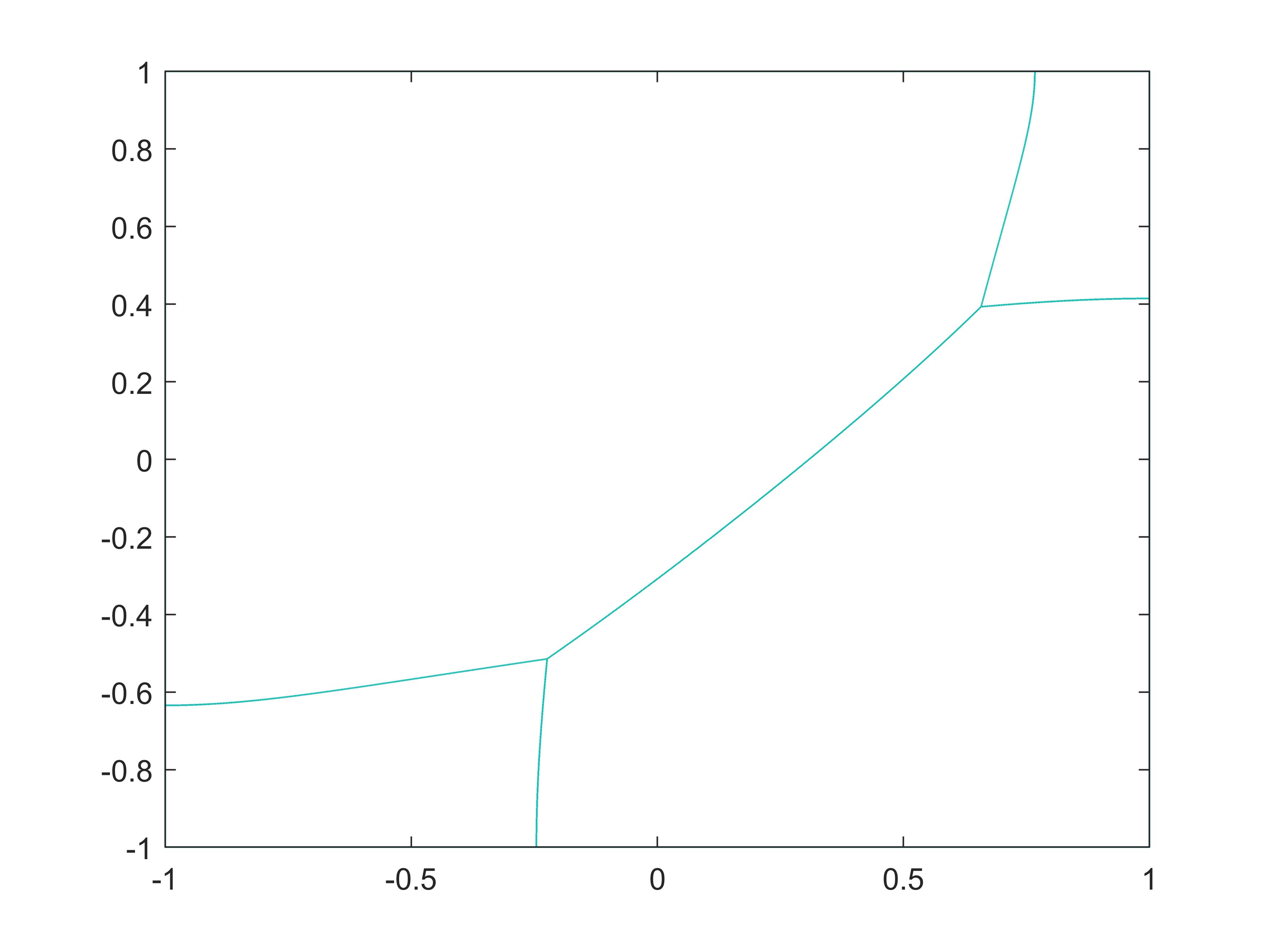 Figure 2
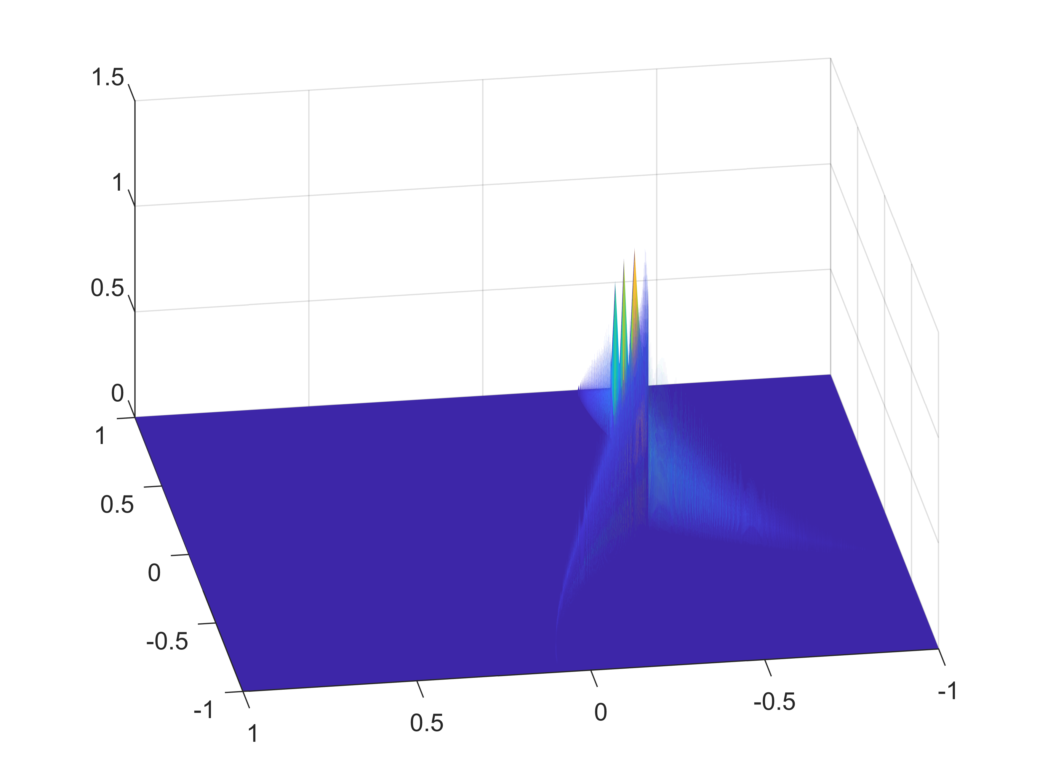 Figure 3
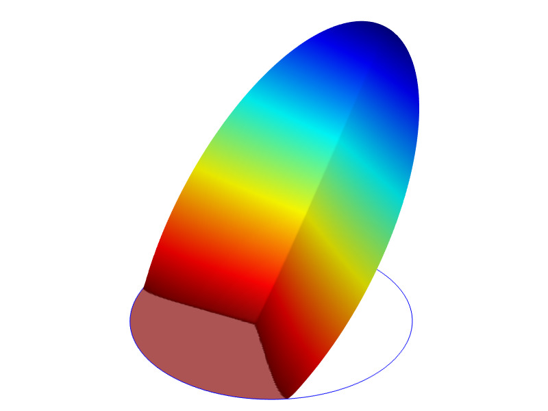 Figure 4
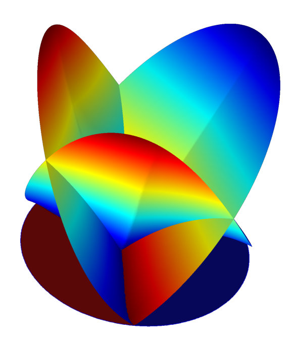 Figure 5
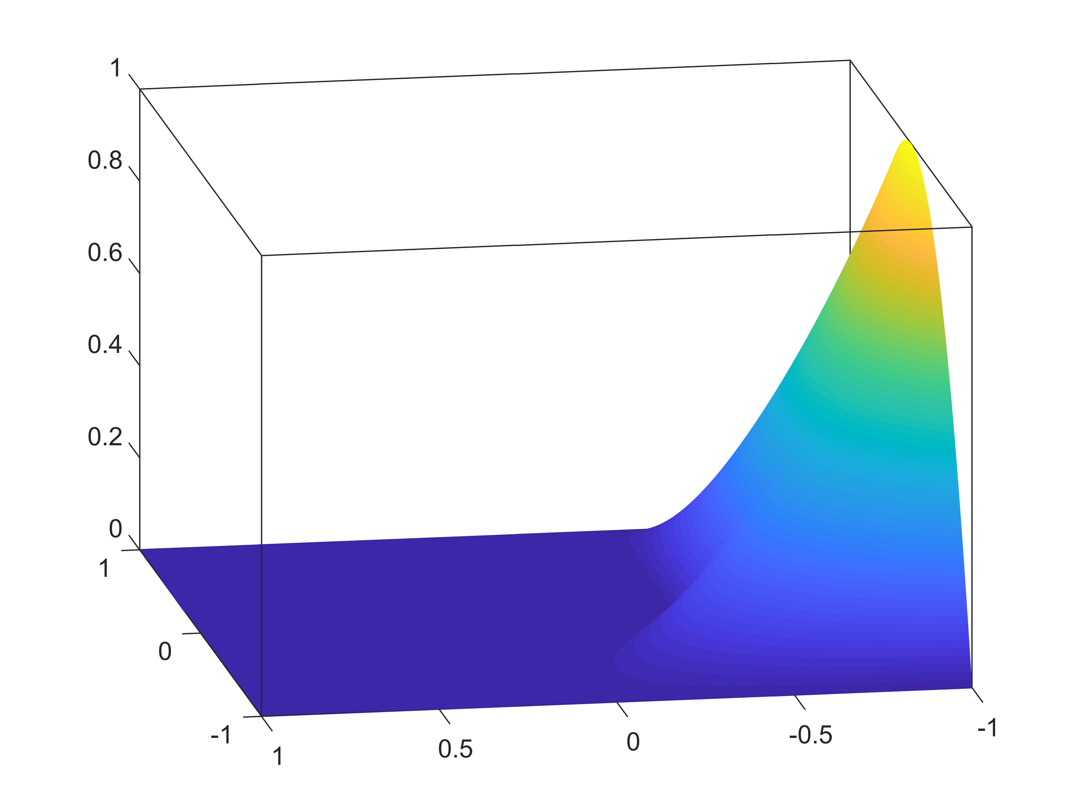 Figure 6
Peer Reviews
No public reviews on file for this paper yet. If you reviewed it on a platform where reviews are public (OpenReview, ICLR, NeurIPS, ICML), you can paste yours below so the community can read it here.
Videos
No videos yet. Explain this paper in a talk, walkthrough, or lecture? Add one.
Taxonomy
TopicsDifferential Equations and Numerical Methods · Advanced Mathematical Modeling in Engineering · Nonlinear Partial Differential Equations
On a Class of Singularly Perturbed Elliptic Systems with Asymptotic Phase Segregation
Farid Bozorgnia, Martin Burger
Department of Mathematics, Instituto Superior Técnico, Lisbon.
Department Mathematik, Friedrich-Alexander Universität Erlangen-Nürnberg, Erlangen (FAU)
Abstract.
This work is devoted to study of a class of elliptic singular perturbed systems and their singular limit to a phase segregating system. We prove existence and uniqueness and study the asymptotic behaviour with convergence to a limiting problem as the interaction rate tends to infinity. The limiting problem is a free boundary problem such that at each point in the domain at least one of the components is zero which implies simultaneously all components can not coexist. We present a novel method, which provides an explicit solution of limiting problem for special choice of parameters. Moreover, we present some numerical simulations of the asymptotic problem.
The corresponding author, F. Bozorgnia was supported by the Portuguese National Science Foundation through FCT fellowships SFRH/BPD/33962/2009
Keywords: Singular perturbed system, segregation, free boundary problems, numerical approximation.
2010 MSC:58J37,35R35, 34K10.
1. Introduction and problem setting
In order to model strong interaction between multiple components with reaction and diffusion, different models have been proposed. Among these models the adjacent segregation models have been extensively studied from different point of views, to see about theoretical aspects we refer to [5, 6, 8, 12]. Most of the works are related to the case of two components, while [5] considers an extension to multiple components with strict segregation. Here we consider a different extension to multiple components that is still consist with the other models for the case of two components, the segregation behaviour is of different type for multiple ones however.
Let be bounded domain with smooth boundary. The model describes the steady state of species diffusing and interacting between all component in Let denote the population density of the component. We study the following singular elliptic system introduced in [6], with unknowns which satisfy
[TABLE]
for . Here the function is given by
[TABLE]
for an -tuple with
The main assumptions on boundary values and data are as below:
Assumption 1**.**
The boundary data are non-negative functions with following partial segregation property
[TABLE]
Assumption 2**.**
The functions are smooth, positive and satisfy
[TABLE]
The system (1.1) and the limiting system for appear in theory of flames and are related to a model called Burke-Schumann approximation. The main assumption in Burke-Schumann model is that oxidizer and reactant mix on a thin sheet and the flame precisely occurs there. A way to justify the underlying assumption is to introduce a large parameter called Damköhler number, denoted by , which is the parameter measuring the intensity of the reaction (see [16]). Then, the a chemical reaction is described by
[TABLE]
Let and , respectively, denote the mass fraction of the oxidizer and the fuel, then they satisfy the following system
[TABLE]
with given incompressible velocity field and a Dirichlet boundary condition on .
In [6] a general Hölder estimate for a class of singular perturbed elliptic system (1.1) is shown. The authors applied this estimate to the well-known Burke-Schumann approximation in flame theory. Also they study the classical cases i,e., equidiffusional case with high activation energy approximation, non- equidiffusional case, and to nonlinear diffusion models. The limiting problems are nonlinear elliptic equations; they have Hölder or Lipschitz maximal global regularity.
We point out that L. Caffarelli and F. Lin in [5] studied the following system with different coupling term
[TABLE]
where the boundary values satisfy
[TABLE]
Remark 1.1*.*
In system (1.1) choosing and
[TABLE]
we get system (1.2) for which has been studied extensively. Thus in (1.1) we are interested when
To see different theoretical aspects of the system (1.2) we refer to [5, 12, 15] and references therein. In [5] the authors study the asymptotic limit; as tends to zero in system (1.2) and they show that limiting case yields to pairwise segregation. Furthermore, it is shown that away from a closed subset of the Hausdorff dimension less or equal the free interfaces between various components are, in fact, smooth hyper surfaces.
For the numerical approximation of the system (1.2) we refer to [3, 4]. In [3] the authors propose a numerical scheme for a class of reaction-diffusion system with densities having disjoint supports and are governed by a minimization problem. The proposed numerical scheme is applied for the spatial segregation limit of diffusive Lotka-Volterra models in presence of high competition and inhomogeneous Dirichlet boundary conditions. In [1] the proof of convergence of the finite difference scheme for a general class of the spatial segregation of reaction- diffusion, is given.
This work is devoted to analyse existence and uniqueness results for system (1.1), as well as a study of the qualitative properties of solutions to (1.1) as tends to zero. A particular novelty of the current work is to provide an explicit solution for an arbitrary number of components when the parameter tends to zero in the following system
[TABLE]
For the cases be same or are constants.
The outline of this paper is as follows: Section 2 consists the proof of existence and uniqueness of system (1.1). Section 3 deals with the limiting case as tends to zero. In Section 4 we give an explicit solution for limiting case together with a rate of convergence. Section 5 provides some numerical simulations of the singular limit.
2. Analysis of the model for fixed
In this section we prove existence and uniqueness of the solution of System (1.1) for fixed . The proof is constructive and we implement it to obtain numerical approximation of (1.3)
Consider the following related time dependent parabolic system
[TABLE]
where in (2.1) the initial values are non-negative and compatible with boundary data. Then by Theorem 2.1 in [10] we obtain
[TABLE]
Also it is straight to show that as tends to infinity
[TABLE]
with being the solution of (1.1), see [7, 11].
Let be a positive solution of the system (1.3) then
[TABLE]
where
[TABLE]
We denote the harmonic extension of boundary data with . We multiply the following equation
[TABLE]
by where Then integrating by parts gives
[TABLE]
Note that the integrand of right hand side is positive and
[TABLE]
From here which implies
[TABLE]
A standard maximum and nonnegativity principle for elliptic equations (cf. [14]) yields the following result. In sequel we use this result.
Lemma 2.1**.**
Let be a weak solution of the system
[TABLE]
with and bounded and nonnegative, then
[TABLE]
where
[TABLE]
In the next Theorem 2.2 we show the existence of nonnegative solutions to the original system. The main idea of the proof is to construct sub and super solution and decoupling the system in iterative way and to exploit the uniform bounds, see also the proof in [15] for the proof of uniqueness of the solution for system (1.2).
Theorem 2.2**.**
For each there exist a unique nonnegative solution
[TABLE]
of the system (1.1).
Proof.
Without loss of generality in the proof we set i.e.,
[TABLE]
To start, consider the harmonic extension given by
[TABLE]
Next, given consider the solution of the following linear system
[TABLE]
Note that we can subsequently solve the equations for increasing due to the triangular structure and always obtain a problem of the form considered in Lemma 2.1, hence the uniform bounds apply. We show that the following inequalities hold:
[TABLE]
The first iteration for reads as
[TABLE]
Note that since and boundary conditions are non negative then the weak maximum principle (see appendix) implies that The equation for in (2.4) is given by
[TABLE]
Repeating the same argument, we obtain that and consequently
[TABLE]
Now we have
[TABLE]
Thus the comparison principle implies that . The same argument shows
[TABLE]
In the next step we verify the following inequalities hold
[TABLE]
To do this, one verifies that inequality holds then this fact can be used to prove inequality for . Then the same arguments show that
[TABLE]
To proceed more with induction, assume that
[TABLE]
We show that
[TABLE]
To show this, first we check for and the same argument can be applied consequently. By (2.4) and the assumption in (2.6) we have
[TABLE]
Note that and have the same boundary value so by the comparison principle
[TABLE]
Now we proceed for . The same argument using the assumption shows that
[TABLE]
For the next step, we use the fact from previous step which states to verify
Now let and be two families of functions such that
[TABLE]
[TABLE]
Taking the limit in (2.4) yields for the followings hold
[TABLE]
The inequality implies that
[TABLE]
We will show that in fact the equality holds. To do this, first consider the equations for the
[TABLE]
which implies
[TABLE]
Now by checking the equation for in (2.7) and using the previous fact yields
[TABLE]
and argument is repeated backward which shows equality for every .
To show uniqueness, assume there exists another positive solution of system, then we show
[TABLE]
We will prove that the following equations hold:
[TABLE]
To begin, we show that
[TABLE]
This is a consequence of the fact that satisfies
[TABLE]
Next we compare with and we show . As in existence part, first we check for in inequality follows from (2.11) and
[TABLE]
Now we proceed by induction and we assume that the claim is true until This means that we have
[TABLE]
Then we show
[TABLE]
Again comparing the equations for and and the using assumption yields the following inequality
[TABLE]
The same reasoning for inequality holds. Now taking limit in (2.10 ) shows that
[TABLE]
∎
3. Limiting problem
In this section we study properties of the solution for system (1.1) to provide estimates and compactness results to pass to the limit as tends to zero.
As we have seen in the last section, for each fixed the system (1.1) has a unique solution. Let be the unique positive solution of system (1.1) for fixed then for satisfy the following differential inequalities:
[TABLE]
Also define as
[TABLE]
then considering the assumption 2, it is easy to verify that
[TABLE]
Let and for be harmonic with boundary value and respectively, where
[TABLE]
then we have
[TABLE]
which implies
[TABLE]
In this part we show that the solution of system (1.1) has bound in independently of To do this, we prove several lemmas.
Lemma 3.1**.**
Assume and . Let satisfies the following
[TABLE]
Then
[TABLE]
for some that only depends on dimension .
Proof.
Without loss of generality, assume . By Green’s formula for ball one has
[TABLE]
[TABLE]
Next, rearranging terms proves the Lemma. ∎
Lemma 3.2**.**
Assume that satisfies
[TABLE]
Then there exists a constant depends only on and such that
[TABLE]
Proof.
The proof consider different cases.
- (1)
If then it follows by previous Lemma 3.1. 2. (2)
If such that on then we may extend to
[TABLE]
and apply the previous Lemma to 3. (3)
If none of vanishes on then, since the product of boundary values is zero, there must be a that vanishes at a point we may assume that Also, since it follows that
[TABLE]
Now let solves
[TABLE]
Since and are it follows that
[TABLE]
Now either satisfies
[TABLE]
for some (which we will decide ) in which case we may apply the previous Lemma on since
[TABLE]
or there is a point such that
[TABLE]
Note that since otherwise,
[TABLE]
provided is large enough. Next, since there is another say , such that Let solves
[TABLE]
Then again in for some depending only on the domain and . Next let in where
[TABLE]
Since is bounded; on then it follows that
[TABLE]
where depends on the bound and . This leads in particular to
[TABLE]
This is a contradiction if is large enough and this complete the proof.
∎
Proposition 3.3**.**
Let be as in previous Lemma. Then there exists a constant (independent of such that
[TABLE]
Proof.
Cover by finitely say balls and notice that
[TABLE]
Next let and define
[TABLE]
Then satisfies
[TABLE]
which implies
[TABLE]
where is chosen so large that Now let where
[TABLE]
Since and by (3.7), then it follows that with bounds only depending on and In particular, is bounded independent of . ∎
The above Lemma shows that up to a subsequence denoted with we get
[TABLE]
The main result of this section is Theorem 3.4 which shows the asymptotic behaviour of system (1.3) as tends to zero.
Theorem 3.4**.**
Let be a solution of the system at fixed . Let tends to zero, then there exists such that for all :
- (1)
* in the sense of distribution.* 2. (2)
up to subsequences, strongly in . 3. (3)
* a.e in *
Proof.
Proposition (3.3) shows the existence of a weak limit such that, up to subsequences,
[TABLE]
The weak limit for satisfy the following differential inequalities
[TABLE]
since we can pass to the weak limit in the differential inequalities for and To show the strong convergence, we show that
[TABLE]
By weak lower semi continuously of Dirichlet norm just needs to show
[TABLE]
We multiply the inequality by and integration by parts,
[TABLE]
This implies
[TABLE]
Next we multiply the equation for by to obtain
[TABLE]
Taking the limit as tends to zero and considering the weak convergence of and previous part to have
[TABLE]
Form (3.9) and (3.10) the result holds.
(2) Fix a point and let the index be such that
[TABLE]
Now assume that then by Hölder continuity there is such that
[TABLE]
Next we use the fact that the functions for are subharmonic, using the mean value property for subharmonic functions (see the proof of theorem 2.1 in [13])
[TABLE]
From here the following holds
[TABLE]
Note that in the ball we have so from (1.3) we obtain
[TABLE]
Next, in (3.13) let tend to zero which yields
[TABLE]
∎
Let be the first eigenfunction of the Laplace operator in i.e.,
[TABLE]
The first eigenfunction does not change the sign and we may therefore take it to be positive and normalized it so that Multiplying the equation
[TABLE]
by and integrating over yields
[TABLE]
Integration by parts and implementing that is zero on boundary, we obtain
[TABLE]
Now from the bound on and the fact that normal derivative of the first eigenfunction on the boundary is bounded, we conclude
[TABLE]
We know that for the solution are Hölder continuous
[TABLE]
where the constant is independent of Note that, since
[TABLE]
then the inequality in above yields that
[TABLE]
where the constant is independent of For the rest, we show that for those points close enough to the boundary, remains bounded. Let and denote the Hölder constant and Hölder exponent of Choose the strip around boundary such that
[TABLE]
Let be a point such that has minimum distance to . Then by assumption on the boundary values, there is such that and
[TABLE]
The previous inequality and (3.15) imply that
[TABLE]
Combining (3.14) and (3.16) yields that Laplace of is bounded.
Remark 3.1*.*
The uniform bound of normal derivative of yields estimates for limiting problem as follows. Integrate from
[TABLE]
to obtain
[TABLE]
From here we get
[TABLE]
this shows
[TABLE]
Definition 3.1**.**
Consider the non empty sets . Then the free boundaries (interfaces) are define as
[TABLE]
In the next Lemma we give the free boundary condition for the case .
Lemma 3.5**.**
The following conditions holds on the free boundary
- (1)
** 2. (2)
**
Proof.
Let be a free boundary point in Note that
[TABLE]
In the sense of distribution we have
[TABLE]
Splitting and considering the fact that in we have the second relation is proved.
∎
Remark 3.2*.*
: In [15] the uniqueness of the limiting solution of system (1.2) for arbitrary number of components, is shown. Consider the metric space defined by
[TABLE]
In [15] (see Theorem 1.6 ) it is shown that the limiting solution of (1.2) is a harmonic map into the space By definition the harmonic map is the critical point of the following energy functional
[TABLE]
among all nonnegative segregated states a.e. with the same boundary conditions.
Also in [2] an alternative proof of uniqueness for limiting case for system(1.2) is given which is more direct and based on properties of limiting solutions. Although some properties of limiting solution for systems (1.3) and (1.2) are similar, the proof of uniqueness for system (1.3) in the case tends to zero remains challenging problem.
Define the energy associated to densities defined by
[TABLE]
Now consider the following problem
[TABLE]
over the closed but non-convex set
[TABLE]
Existence of a minimizer is direct. The following variation
[TABLE]
with yields the following
[TABLE]
This implies that each is harmonic in its support which dose not hold for our limiting solution. In fact, for system (1.3) in Theorem 3.2 we show that
[TABLE]
Figure 1 also shows is not smooth in its support are Dirac measures on interfaces.
4. Explicit solutions in the limiting case
In this section we give an explicit solution and the rate of convergence for the limiting solution of the following system
[TABLE]
for the cases that are the same or constants.
4.1. Construction of Solutions
It is easy to check that for every
[TABLE]
which remains true as tends to zero. First of all define
[TABLE]
then is the harmonic extension of the Dirichlet value This means that for is the solution of
[TABLE]
Note that the nonnegativity of the is equivalent to . Thus, an obvious candidate solution is given by
[TABLE]
and
[TABLE]
Obviously, by this construction we have and moreover
[TABLE]
To see the latter, let be fixed and such that for all . Then
[TABLE]
We finally need to verify . For this follows from the fact that maximum of harmonic function is subharmonic then for the rest of it follows from (4.4) and (4.5).
Remark 4.1*.*
Let be defined as below :
[TABLE]
then set
[TABLE]
From this we can recover other components by
[TABLE]
One can check this choice gives the same solutions as in (4.4) and (4.5), for the case is straightforward.
4.2. Convergence Rate
We now turn our attention to a rate of convergence of the solutions as . Note that
[TABLE]
is harmonic with Dirichlet data , hence coincides with the one in the previous section, in particular independent of .
We thus have
[TABLE]
Now we have and , hence
[TABLE]
respectively
[TABLE]
Applying Young’s inequality on the right-hand side we deduce
[TABLE]
5. Numerical Study of the Limiting Problem
This section provides some examples of numerical approximations to the limiting problem of the following system.
[TABLE]
In our examples we implemented directly mimicking the fixed point technique in the existence proof of Theorem 2.2 with value of and the method in Section 4 which demonstrate those give basically the same as epsilon goes to zero
Example 5.1**.**
Let The boundary values for are defined by
[TABLE]
[TABLE]
Here the boundary conditions satisfy
[TABLE]
The surface of is depicted in Figure 1. Also one can check the jump in gradient of along which has shown in part 2 of Lemma (3.5). In Figure 2,
Example 5.2**.**
Let and The boundary values (i=1,2,3,4) are given as follows:
[TABLE]
[TABLE]
We implemented the iterative scheme given by Lemma 2.2 with and method given by (4.4) and (4.5). The obtained solutions are same and the surface of is given in (6).
The interfaces are shown in Figure LABEL:fig5.
In Figure (5 we draw the Laplace of on the interfaces. We know Laplace of is Dirac along interfaces so we scaled by multiplying by mesh size.
Example 5.3**.**
Next, we change boundary values as below.
[TABLE]
[TABLE]
The following picture shows the interfaces
The reference list from the paper itself. Each links out to its DOI / PubMed record.
- 1[1] A. Arakelyan Convergence of the finite difference scheme for a general class of the spatial segregation of reaction–diffusion systems. Computers and Mathematics with Applications, 75, (2018) 4232-4240.
- 2[2] A. Arakelyan, F. Bozorgnia, On the uniqueness of the limiting solution to a strongly competing system. Electronic Journal of Differential Equations, 96, (2017) 1-8.
- 3[3] F. Bozorgnia, A. Arakelyan, Numerical algorithms for a variational problem of the spatial segregation of reaction-diffusion systems. Applied Mathematics and Computation 219 (17), 8863-8875.
- 4[4] F. Bozorgnia, Numerical algorithms for the spatial segregation of competitive systems. SIAM J. Sci. Comput, 31, (2009) 3946-3958.
- 5[5] L. Caffarelli, F. Lin, Singularly perturbed elliptic systems and multi-valued harmonic functions with free boundaries. J. Amer. Math. Soc. 21, no. 3, (2008) 847–862.
- 6[6] L. Caffarelli and J. Roquejoffre, Uniform Hölder estimate in a class of elliptic systems and applications to singular limits in models for diffusion flames. Arch. Ration. Mech. Anal. 183, no. 3, (2007) 457–487.
- 7[7] E. C. M. Crooks, E. N. Dancer and D. Hilhorst, On long-term dynamics for competition-diffusion system with inhomogeneous dirichlet boundary conditions. Topological Methods in Nonlinear Analysis, 30, (2007) 1-36.
- 8[8] E.N. Dancer, Y.H. Du, Competing species equations with diffusion, large interactions, and jumping nonlinearities , J. Differential Equations. 114, (1994) 434-475.