Variable Demand and Multi-commodity Flow in Markovian Network Equilibrium
Yue Yu, Dan Calderone, Sarah H. Q. Li, Lillian J. Ratliff and, Beh\c{c}et A\c{c}{\i}kme\c{s}e

TL;DR
This paper extends Markovian network equilibrium to include variable demand with quitting options and multi-commodity flows with heterogeneous ending times, providing new algorithms and computational analysis.
Contribution
It introduces two novel extensions to Markovian network equilibrium and develops dynamic programming algorithms with complexity analysis.
Findings
Algorithms outperform Mosek in computational efficiency.
Extensions handle variable demand and multi-commodity flows.
Numerical experiments validate the proposed models.
Abstract
Markovian network equilibrium generalizes the classical Wardrop equilibrium in network games. At a Markovian network equilibrium, each player of the game solves a Markov decision process instead of a shortest path problem. We propose two novel extensions of Markovian network equilibrium by considering 1) variable demand, which offers the players a quitting option, and 2) multi-commodity flow, which allows players to have heterogeneous ending time. We further develop dynamic-programming-based iterative algorithms for the proposed equilibrium problems, together with their arithmetic complexity analysis. Finally, we illustrate our network equilibrium model via a multi-commodity ride-sharing example, and compare the computational efficiency of our algorithms against state-of-the-art optimization software Mosek over extensive numerical experiments.
Click any figure to enlarge with its caption.
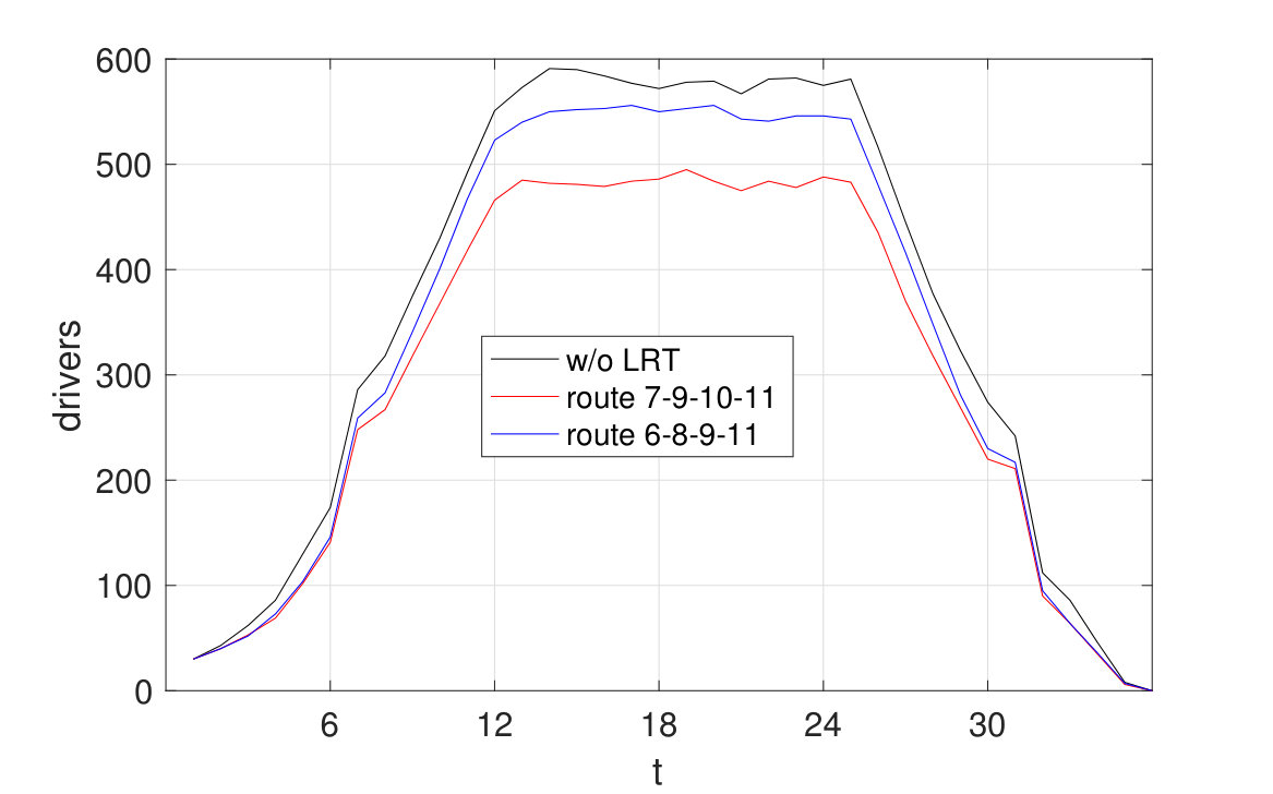 Figure 1
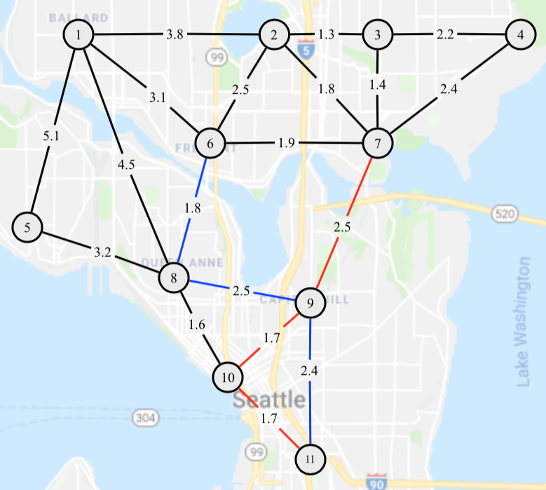 Figure 2
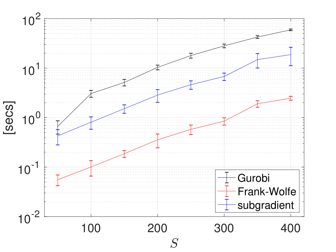 Figure 3
|
|
|
|
|
|
|---|---|---|---|---|
| 600 | 200 | 60 | 60 | |
| 200 | 400 | 200 | 60 | |
| 60 | 100 | 600 | 60 |
Peer Reviews
No public reviews on file for this paper yet. If you reviewed it on a platform where reviews are public (OpenReview, ICLR, NeurIPS, ICML), you can paste yours below so the community can read it here.
Videos
No videos yet. Explain this paper in a talk, walkthrough, or lecture? Add one.
Taxonomy
TopicsTransportation and Mobility Innovations · Transportation Planning and Optimization · Urban Transport and Accessibility
Variable Demand and Multi-commodity Flow in Markovian Network Equilibrium
Yue Yu
Dan Calderone
Sarah H. Q. Li
Lillian J. Ratliff
Behçet Açıkmeşe
Oden Institute for Computational Engineering and Sciences, The University of Texas at Austin, Austin, TX, 78712
Department of Aeronautics and Astronautics, University of Washington, Seattle, WA, 98195
Department of Electrical and Computer Engineering, University of Washington, Seattle, WA, 98195
Abstract
Markovian network equilibrium generalizes the classical Wardrop equilibrium in network games. At a Markovian network equilibrium, each player of the game solves a Markov decision process instead of a shortest path problem. We propose two novel extensions of Markovian network equilibrium by considering 1) variable demand, which offers the players a quitting option, and 2) multi-commodity flow, which allows players to have heterogeneous ending time. We further develop dynamic-programming-based iterative algorithms for the proposed equilibrium problems, together with their arithmetic complexity analysis. Finally, we illustrate our network equilibrium model via a multi-commodity ride-sharing example, and compare the computational efficiency of our algorithms against state-of-the-art optimization software Mosek over extensive numerical experiments.
keywords:
Wardrop equilibrium, Markov decision process, network optimization
, , , ,
††thanks: Y. Yu is with the Oden Institute for Computational Engineering and Sciences, The University of Texas at Austin, Austin, Texas, 78712 (e-mail: [email protected]). S. H. Q. Li, and B. Açıkmeşe are with the William E. Boeing Department of Aeronautics & Astronautics, University of Washington, Seattle, Washington, 98195 (e-mail: [email protected], [email protected], [email protected]). D. Calderone and L. J. Ratliff are with the Department of Electrical & Computer Engineering, University of Washington, Seattle, Washington, 98195 (e-mail:[email protected], [email protected]).
1 Introduction
Network equilibrium problems arise in a variety of applications, such as resource allocation and routing in communication or transportation networks [Rockafellar, 1984, Bertsekas, 1998, Xiao et al., 2004, Bürger et al., 2014]. Among the most well-studied examples is the Wardrop equilibrium model in routing games [Beckmann et al., 1956, Gartner, 1980a, Gartner, 1980b, Correa and Stier-Moses, 2010, Patriksson, 1994]. In this model, users in a transportation network are assumed to choose routes with cost that they perceive as the lowest, i.e., each user solves a shortest path problem, under the prevailing traffic conditions [Correa and Stier-Moses, 2010]. With this assumption, the resulting equilibra are characterized by the Wardrop equilibrium principle: the cost of all the routes actually used are equal, and less than those which would be experienced by a single user on any unused route [Wardrop and Whitehead, 1952].
To ensure their practical relevance, it is often necessary to incorporating stochasticity into the network equilibrium problems. For example, the stochastic user equilibrium (SUE) model [Fisk, 1980, Sheffi and Powell, 1982, Liu et al., 2009] considers independent stochastic error on the route cost perceived by the users, leading to user distribution based on the logit [Dial, 1971] or probit model [Daganzo and Sheffi, 1977]; see [Patriksson, 1994, Sec. 2.8.1] and [Cominetti et al., 2012] for a detailed discussion. Unfortunately, the SUE model presents several drawbacks: it requires computationally expensive route enumeration, and is not suited for problems with overlapping routes due to its assumption of independent route cost.
To address these drawbacks, different network models consider different type of stochasticity. In particular, [Baillon and Cominetti, 2008, Ahipaşaoğlu et al., 2019] introduced a Markovian network equilibrium model where users are assumed to choose, instead of routes, sequences of actions with accumulated cost that they perceive as the lowest. Each action is accompanied by a deterministic outcome and a stochastic cost. For example, each vehicle in a transportation network is assumed to choose a sequence of arcs, where each arc leads to deterministic transition to the next node in the network and a stochastic amount of travel time [Baillon and Cominetti, 2008].
On the other hand, [Calderone and Sastry, 2017b, Calderone and Sastry, 2017a] proposed a different stochastic network equilibrium model. Unlike the one in [Baillon and Cominetti, 2008], each action is accompanied by a stochastic outcome and a deterministic cost. For example, an aircraft flying in stormy weather is assumed to choose a sequence of waypoints to fly towards, where each choice costs a deterministic amount of fuel usage and is accompanied by a stochastic change in the weather condition [Nilim and El Ghaoui, 2005]. As a result, instead of a shortest path problem, each user solves a Markov decision process (MDP) [Puterman, 1994, Bertsekas, 1996], where the cost of different actions is determined by the prevailing choices of all users. This model has found a variety of applications in modern transportation including ridesharing and parking [Calderone, 2017].
Although the results in [Calderone and Sastry, 2017b, Calderone and Sastry, 2017a] serves as a first step toward a more general class of stochastic dynamic network equilibrium model, it has the following limitations: a) it does not incorporate many important features of Wardrop equilibrium, such as variable demand and multi-commodity flow and b) its solution method relies exclusively on off-the-shelf optimization software, which does not fully exploit the problem structure. We address these limitations by making the following contributions.
We develop novel extensions to the Markovian network equilibrium model by considering a) variable demand, which offers the users a quitting option, and b) multi-commodity flow, which allows users having heterogeneous ending time. 2. 2.
We design novel dynamic-programming-based algorithms for Markovian network equilibrium problems with detailed arithematical complexity analysis. Our algorithms outperform state-of-the-art optimization software Mosek in extensive numerical experiments.
The rest of the paper is organized as follows. We first revisit some background on MDP in Section 2, then present our variable demand and multi-commodity flow equilibrium models in Section 3. Section 4 focuses on developing efficient iterative algorithms for our equilibrium problems. Section 5 first illustrates the equilibrium models in Section 3 via a multi-commodity ride-sharing example, then compares the algorithms in Section 4 against commercial software Mosek. Finally, we conclude with discussions and comments on the future directions of research in Section 6.
Throughout the paper we will use the following notation: denotes the set of real numbers, denotes the set of nonnegative real numbers, and denotes the set of positive integers; denotes the set for integer ; denotes the –th component of the three-dimensional tensor , and analogously, for the two-dimensional case. Given , we say if and .
2 Preliminaries and background
A -horizon MDP is defined by a set of states , a set of actions , a cost tensor , and a transition probablity tensor , where denote the number of time steps, states, and actions, respectively. Further, denotes the cost of choosing action in state at time , and denotes the probability of transition from state to when choosing action . In order to find the optimal sequence of action that minimizes the expected accumulated cost, one can solve either one of the two following linear programs111Compared with the formulation in [Puterman, 1994], the linear program here also allows when .:
[TABLE]
[TABLE]
where is such that for some . If and for all and , then represents the probability of starting the MDP in state . Variable in optimization (1) represents the probability of choosing action in state at time , and variable in optimization (2) represents the expected accumulated cost between time and time starting from state . In general, optimization (1) and (2) can be interpreted as the linear optimal distribution [Rockafellar, 1984, Sec.7A] and differential problem [Rockafellar, 1984, Sec.7E] defined on a -layered Markovian network (see Fig. 1), where represents the divergence on state node in the -th layer, represents the flow from state to action in the -th layer, and represents the potential on state in the -th layer.
The following lemma shows that solutions of optimizations (1) and (2) satisfy the dynamic programming principle.
Lemma 1** ([Puterman, 1994]).**
Suppose solves (1), and solves (2). If for any , then
[TABLE]
for all .
Perhaps the most efficient solution algorithm for problem (1) and (2) is dynamic programming, given by the following Algorithm 1 and Algorithm 2.
Let be the output of Algorithm 1 with input , and be the output of Algorithm 2 with input , then one can easily show that such solution pair directly satisfies the Karush-Kuhn-Tucker (KKT) conditions [Rockafellar, 1970, Thm. 28.3] of (1) and (2), hence it is an optimal primal-dual solution pair. If we define the sparsity level of an MDP as follows
[TABLE]
where N_{1}=\max_{s,a}\big{|}\{s^{\prime}|P_{sas^{\prime}}>0\}\big{|} and N_{2}=\max_{s^{\prime},a}\big{|}\{s|P_{sas^{\prime}}>0\}\big{|}, then measures the maximum number of states connected by the transition kernel . Further, it is straightforward to check that Algorithm 1 costs arithmetic operations, and Algorithm 2 costs arithmetic operations. In addition, Algorithm 1 and Algorithm 2 can be implemented as convolutional neural networks that allows efficient parallel computation [Tamar et al., 2016].
3 Markovian network equilibrium
By combining MDP together with classical routing games, Calderone and Sastry [Calderone and Sastry, 2017b] proposed MDP routing games where a fixed amount of players with the same planning horizon choose sequences of actions that they perceive as achieving the lowest expected accumulated cost under the prevailing choices of other players. Such games are similar to routing games where a fixed amount of players with the same destination choose routes that they perceive as the shortest under the prevailing choices of other players.
In this section, we introduce two generalizations to MDP routing games that allow the amount of players to vary and the planning horizon to differ. We will also show that, under mild assumptions, the equilibra of such games can be computed efficiently using convex optimization.
3.1 Variable demand
One limitation of the MDP routing games in [Calderone and Sastry, 2017b] is the assumption that total amount of players is fixed. However, an important feature in network games is to allow the total amount of players to vary, or equivalently, to provide the players with a quitting action [Patriksson, 1994, Sec. 2.1.2]. Aiming to address this limitation, we propose the following variable demand MDP routing games.
Game 1**.**
At each time , new players start the game from state . Among these players, each one can choose to
quit the game immediately at the cost of , 2. 2.
take action at the cost of and reach state with probability at time , then repeat such process till , when the player ends the game after choosing the last action,
where and denote the total amount of players choosing to quit the game in state at time , and, respectively, taking action in state at time .
Remark 1**.**
Game 1 is a special case of mean field games over graphs [Gomes et al., 2009, Gomes et al., 2010, Guéant, 2011, Guéant, 2015, Tanaka et al., 2020]. The interactions among different players is mediated by a mean field, described by function and function for all .
Intuitively, one can interpret Game 1 as a competitive market model. The supply side corresponds to the stochastic environment, providing the option of playing or quitting the game. The demand side corresponds to the amount of players that decided to play the game, which changes with the expected accumulated cost of the playing option according to curve for all and .
Remark 2**.**
If the quitting option is not available, then Game 1 reduces to an MDP routing game with fixed demand, introduced in [Calderone and Sastry, 2017b]. On the other hand, if the transition is Game 1 is deterministic, i.e., for each and , there exists such that , then Game 1 reduces to a classical single-commodity routing game, with and a variable demand [Patriksson, 1994, Sec. 2.2.3]. Particularly, each player solves an MDP with deterministic transition, which is equivalent to a shortest path problem.
The Wardrop equilibrium principle is a key characterization of the equilibra of network games [Patriksson, 1994, Correa and Stier-Moses, 2010]. The principle states that, at equilibra, only the strategies with the lowest cost are actually used. Does this principle apply to Game 1? As we show in the following, the answer is affirmative.
First, we make the following assumptions on Game 1.
Assumption 1**.**
We assume that , and for all , . Further, the function and function are continuous and strictly increasing over their respective domains, where .
With these assumptions, we now introduce the following pair of primal-dual optimization problems associated with Game 1.
[TABLE]
[TABLE]
In particular, the constraint allows the number of players choosing to quit the game in state at time to vary winthin interval . If variable is zero and function is constant-valued for all , i.e., the quitting option is removed and the cost of each action does not depend on in in Game 1, then one can verify that optimization (4) will reduce to (1) and optimization (5) will reduce to (2).
The following theorem shows that, under Assumption 1, the solution to the optimizations in (4) and (5) satisfy an equilibrium condition of Game 1. Similar to the Wardrop equilibrium principle, this equilibrium condition impliesthat no individual player can benefit from unilaterally switching its actions.
Theorem 1**.**
Suppose Assumption 1 holds, solves (4), and solves (5), then for any ,
[TABLE]
Further, if , then
[TABLE]
for all .
{pf*}
Proof See Appendix A.1.
Theorem 1 shows that an equilibrium of Game 1 that satisfies the Wardrop equilibrium principle not only exists, but can be computed by solving optimization (4) and (5). In particular, if action is chosen in state at time by any player at equilibrium, i.e., , then action must be optimal in the sense of Algorithm 1. On the other hand, equation (6) says that if some players choose the quitting option in state at time at equilibrium, i.e., , then the cost of playing is no more than quitting, i.e., . Similarly, if some players choose to play, i.e., , then the cost of playing is no more than quitting, i.e., . Therefore, Theorem 1 indeed describes a Wardrop equilibrium where no individual player can benefit from unilaterally switching to alternative actions.
3.2 Multicommodity flow
Another limitation of the MDP routing games in [Calderone and Sastry, 2017b] is that all players are assumed to end their game at the same time, which is analogous to the single commodity routing game where all vehicles have the same destination. Aiming to address this limitation, we propose the following multi-commodity MDP routing game, where players can have heterogeneous ending time, denote by . We assume, without loss of generality, that and .
Game 2**.**
At each time , new players who have a common ending time with , start the game from state . Each of these players can choose the action at the cost of and reach state with probability at time , then repeat this process till , when the player ends the game after choosing the last action. Here denotes the total amount of players who plan to end the game at time and choose action in state at time .
Remark 3**.**
If , then Game 2 reduces to a MDP routing game introduced in [Calderone and Sastry, 2017b]. On the other hand, if the transition in Game 2 is deterministic, i.e., for each and , there exists such that , then Game 2 reduces to the traditional multi-commodity routing game with a fixed demand [Patriksson, 1994, Sec. 2.1.1]. Particularly, the state where a player start and end the game form a origin-destination pair, which is jointly determined by the starting state and the deterministic transition.
Similar to Game 1, the equilibrium of Game 2 can also be computed by solving convex optimization problems, as we show in the following.
First, we make the following assumptions on Game 2.
Assumption 2**.**
We assume , for all , and ; and for all , . Further, the function is continuous and strictly increasing, where .
With these assumptions, we now introduce the following pair of primal-dual optimization problems associated with Game 2. Notice that if , then they reduce to optimization (1) and (2), respectively.
[TABLE]
[TABLE]
The following theorem shows that, under Assumption 2, the solutions to optimization problems (8) and (9) satisfy the equilibrium condition of Game 2. Similar to the Wardrop equilibrium principle, this equilibrium condition implies that no individual player can benefit from unilaterally switching actions.
Theorem 2**.**
Suppose Assumption 2 holds, solves (8), and solves (9). If for any , then
[TABLE]
for all .
{pf*}
Proof See Appendix A.2.
Theorem 2 shows that a Wardrop equilibrium of Game 2 not only exists, but can be found by solving optimization problems (8) and (9). In particular, the equations in (10) characterize a multi-commodity flow Wardrop equilibrium in the sense that no individual player can benefit from using alternative actions before his/her ending time for all .
4 Efficient algorithms via linearization
In this section, we develop efficient iterative algorithms for the network equilibrium problems introduced in the previous section. In particular, we first prove that the linearized versions of problem (4) and problem (8) can both be solved in closed form via Algorithm 1 and Algorithm 2. This observation motivates efficient iterative algorithms that enjoy detailed arithematical complexity analysis.
We will use the following notation to simply our later discussions. Given and , we let and be such that
[TABLE]
for all . We also let and be such that
[TABLE]
for all .
4.1 Linearization and dynamic programming
If we approximate the objective function in (4) using its linearization at and , we obtain the following
[TABLE]
Observe that the above optimization is a modification to problem (1), by including an additional variable . This suggest that (13) may also be solved using dynamic programming, which is confirmed by the following lemma.
Lemma 2**.**
Suppose Assumption 1 holds. Let be the output of Algorithm 1 with input , and
[TABLE]
In addition, let be the output of Algorithm 2 with input . Then
[TABLE]
Further, for any and ,
[TABLE]
{pf*}
Proof See Appendix A.3.
Similarly, if we approximate the objective function in (8) using a linear function, we obtain the following
[TABLE]
where is the approximation parameter, is the optimal value of (14). The following lemma shows that optimization (14) can be solved using Algorithm 1 and 2 as well.
Lemma 3**.**
Suppose Assumption 2 holds. Let be the output of Algorithm 1 with input , be the output of Algorithm 2 with input . Then
[TABLE]
Further, for any ,
[TABLE]
{pf*}
Proof See Appendix A.4.
Remark 4**.**
Function in Lemma 2 is the support function of a polyhedron, which is closed and convex [Rockafellar, 1970, p.28]. Further, Lemma 2 shows that the slope of a linear underestimator, or subgradient, of function can be computed using Algorithm 1 and Algorithm 2. Similar observation is made in Lemma 3 for function .
4.2 Iterative algorithms using linearization
We now develop iterative algorithms for optimization problems in Section 3 using the results from the previous subsection. We will use the following notion of -optimal solution.
Definition 1**.**
Given a constrained optimization where an objective function is optimized subject to constraints, we say a solution is -optimal if it satisfies all the constraints and the objective function value evaluated at this solution is at most away from the optimal value.
We will also use the following additional assumptions on Game 1 and, respectively, Game 2.
Assumption 3**.**
Function and are -Lipschitz continuous over their respective domains for all , and .
Assumption 4**.**
Function is -Lipschitz continuous over its domain for all , and .
Remark 5**.**
Assumption 3 and Assumption 4 are mild assumptions on the differentiability of the corresponding functions. For example, if is continuously differentiable, then the mean value theorem states that for any , there exists such that
[TABLE]
where is the derivative of function . Hence Assumption 4 is satisfied by choosing
[TABLE]
which takes a bounded value since is continuous. However, the continuity of is not necessary. For example, if is a piecewise linear function, i.e., a function that is affine over a collection of intervals, then it is still Lipschitz continuous even if its derivative is not continuous.
Based on Lemma 2 and Lemma 3, we propose to solve optimiztaion (4) and (8) using Frank-Wolfe method [Frank and Wolfe, 1956], which repeatedly solve the linearized versions of (4) and (8). We summarize the Frank-Wolf method for optimization (4) and (8) in Algorithm 3 and, respectively, Algorithm 4. The following theorem provides the overall arithmetic complexity analysis of Algorithm 3 and Algorithm 4.
The following theorem shows the convergence property of Algorithm 3 and Algorithm 4.
Theorem 3**.**
Let be given by (3). If Assumption 1 and 3 hold, then Algorithm 3 with gives an -optimal solution to (4) in arithmetic operations. Similarly, if Assumption 2 and 4 hold, then Algorithm 4 with gives an -optimal solution to (8) in arithmetic operations.
{pf*}
Proof See Appendix A.5.
Theorem 1 provides arithmetical complexity of Algorithm 3 and 4, which not only depends on the problem size (i.e., ), but also the sparsity of the constraints (i.e., ) in (4) and (8).
What about the dual problems? Observe that the optimization in (5) can be separated into two layers: an outer layer that optimizes over , and an inner layer that optimizes over for a given value of ; namely, (5) is equivalent to the following
[TABLE]
where
[TABLE]
One can show that optimization (16) is exactly the dual problem of (13). Since the constraint sets in (13) and (16) are both nonempty, the optimal value of (13) and (16) are the same [Von Neumann and Morgenstern, 1953]. In other words, (5) can be equivalently written as follows
[TABLE]
Using similar reasoning, we can rewrite (9) as follows
[TABLE]
We already discussed in Remark 4 how the subgradients of function and can be computed efficiently using Algorithm 1 and Algorithm 2. In addition, all the other terms in the objective functions of problem (17) and (18) are continuously differentiable. This suggest that (17) and (18) are suited for the projected subgradient method, which optimizes a non-smooth function by repeatedly computing its subgradients and projections onto its domain. We summarize the projected subgradient method applied to (17) and (18) in Algorithm 5 and, respectively, Algorithm 6.
The following theorem shows the the convergence property of Algorithm 5 and Algorithm 6.
Theorem 4**.**
Let be given by (3). If Assumption 1 and Assumption 3 hold, then Algorithm 6 with gives an -optimal solution to (17) using arithmetic operations. Similarly, if Assumption 2 and Assumption 4 hold, then Algorithm 6 with gives an -optimal solution to (18) in arithmetic operations.
{pf*}
Proof See Appendix A.6
5 Numerical examples
In this section, we first illustrate the equilibrium models in Section 3 using a ride-sharing example, then demonstrate the efficiency of algorithms in Section 4 by comparing them against commercial software Mosek (https://www.mosek.com) over extensive numerical experiments.
5.1 Multicommodity ride-sharing game
We consider the game played by ride-sharing drivers in Seattle, competing for customers. We first abstract the Seattle area as an undirected graph illustrated in Fig. 2, whose nodes denote various neighborhoods in Seattle, and edges denote available routes, labeled by its driving distance. We denote the set of neighboring nodes of node as . We model the decision-making of an ride-sharing driver on a typical weekend night (7pm-1am) as an MDP defined as follows.
- •
Time steps: denotes the (end of) 10-minute-intervals between 7pm and 1am.
- •
States: correspond to different nodes in graph .
- •
Actions: in state , denotes picking up a waiting rider with destination for all ; denotes waiting for a future rider.
- •
Transition kernel: we assume is given by
[TABLE]
All other entries of are zero. Here we use an uniform distribution over neighboring states to describe the uncertain destinations of future riders222Such distribution can be approximated more accurately using historical data in practical applications..
- •
Cost: due to the competition among drivers, we assume the profit for picking up a rider decreases with the amount of drivers making the same offer, namely
[TABLE]
for all , where and is the baseline profit and, respectively, nominal profit per mile. We let denotes distance(miles) between and , denotes the rider demand from to at time , and finally denotes the amount of drivers choosing action in state at time . The cost of action in state is a function of defined as follows
[TABLE]
- •
Planning time windows: We assume that 10 drivers start working from each state every 10 minutes between 7pm and 9pm. Once started, each driver is assumed to only work for 4 consecutive hours to avoid driver fatigue, i.e., for all and .
Notice that the function defined above is linear with slope , hence Assumption 2 is satisfied with . In general, as long as is modeled or approximated as a continuously differentiable function, Assumption 4 is always satisfied, as we discussed in Remark 5. We also assume that each driver can travel between neighboring nodes within one time step in this simplified transportation network. In practice, such assumption can be ensured by adding more nodes to the network using a finer discretization of the interested area.
Notice that since drivers can start the game at different times during and they will only plan for the next 24 time steps. In other words, drivers with heterogeneous planning time windows will coexist in the network for . Therefore the equilibrium of this game is a multi-commodity Markovian network equilibrium discussed in Section 3.2. We consider the scenario where , is given in Table 1 and is given in Fig. 2. We compute the driver number in the downtown area by solving the optimization in (8) using commercial software Mosek (https://www.mosek.com). The results are demonstrate in Fig. 3, where we can see that the driver number increases during , then decreases during . There are also two sudden changes in the increasing/decreasing rate around and , which is due to the corresponding changes in values of in Table 1. This example extends the single commodity case considered in [Calderone and Sastry, 2017b] and [Li et al., 2019] where all players enter and exit the game simultaneously.
A relevant application of the above simulation framework is transportation network design. For example, suppose that Seattle city council is considering two candidate light rail transit (LRT) routes, 7-9-10-11 and 6-8-9-11 (see Fig. 2), as a means to alleviate the congestion caused by the ride-sharing traffic in downtown area, assuming that the LRT will reduce the demand of ride-sharing services (namely, value of ) by along its route. The simulated equilibrium with different LRT routes are also given in Fig. 3, which shows that route 6-8-9-11 is more effective that route 7-9-10-11 in terms of reducing amount of drivers in . These results clearly demonstrate the power of Markovian network equilibrium model in transportation system design.
5.2 Computation experiments
To demonstrate the efficiency of the algorithms developed in Section 4, we compare the computation time of our algorithms against commercial software Mosek, used in the previous section, over randomly generated examples. We use to denote a random number sampled from uniform distribution over interval where and .
- •
for all , then normalized such that
- •
for all .
- •
for all if and zero otherwise.
In the variable demand case, we let for all . In the multi-commodity flow case, we let .
We fix and let range between and , then test the computation time of Algorithm 3, Algorithm 5, Algorithm 4 and Algorithm 6, where all algorithms terminate when their objective function value agrees with the optimal one obtained by Mosek with less than relative error. The average computation time over 100 examples, along with corresponding 3-standard deviation interval are reported in Fig. 4. All codes are in MATLAB and run on a 1.6GHz laptop. From results in Fig. 4 we can see that, over the randomly generated 2000 examples, subgradient method and Frank-Wolfe method reduces the computation time consumed by Mosek by one and, respectively, two orders of magnitudes, at the price of a mere of relative accuracy.
6 Conclusion
We study the variable demand and multi-commodity extensions in Markovian network equilibrium. We also propose efficient algorithms that outperform state-of-the-art commercial optimization software. However, the current work still has several limitations. For example, the cost of actions perceived by the players is assumed to be exact, rather than corrupted by stochastic noise, as considered in stochastic user equilibrium model. Further, the ending time of each player is fixed at the beginning of the game. A more realistic assumption is to allow the players to change their ending time and recompute the equilibrium periodically. We aim to address these limitations in future work.
Appendix A Appendix
A.1 Proof of Theorem 1
The objective function of problem (4) is convex (since and are strictly increasing), its constraints are affine, and the optimal value is obviously finite (since and are finitely valued). These imply that a solution pair to (4) and (5) necessarily satisfy the KKT conditions [Rockafellar, 1970, Thm. 28.3.1]. Let be the dual variable corresponding to the equality constraint containing , let be the dual variables corresponding to constraint , and, respectively, . Then the Lagrangian of (4) and (5) is given by
[TABLE]
The KKT conditions [Rockafellar, 1970, Thm.28.3] of this Lagrangian include the following vanishing gradient conditions (by setting equal to zero)
[TABLE]
for all , and the complementarity conditions
[TABLE]
Combining (A.1) and (A.2) yields (6) and (7). Note that same results can be derived from the dual problem (5).
A.2 Proof of Theorem 2
The objective function of problem (8) is convex (since is increasing), its constraints are affine, and the optimal value is obviously finite (since is finitely valued).These imply that a solution pair to (8) and (9) necessarily satisfies the KKT conditions [Rockafellar, 1970, Cor. 28.3.1]. Let be the dual variable corresponding to the equality constraints containing , let be the dual variables corresponding to constraint . Then the Lagrangian of (8) and (9) is given by
[TABLE]
The KKT conditions [Rockafellar, 1970, Thm.28.3] of this Lagrangian include the following vanishing gradient conditions (by setting equal to zero)
[TABLE]
for all , and the complementarity conditions
[TABLE]
for all . Combining (A.3) and (A.4) yields (10). Again, same results can be derived from the dual problem (9).
A.3 Proof of Lemma 2
Using a similar argument as in the proof of Theorem 1, we can show that the KKT conditions of (13) are given by the following
[TABLE]
for all . Let be the output of Algorithm 1 with input , , be the output of Algorithm 2 with input , let
[TABLE]
for all . Then it is straightforward to verify that satisfies all the KKT conditions in (A.5), hence solves (13), which proves the equality. The inequality follows from the fact that, when in (13) is perturbed to another value , solution is still feasible, but can be suboptimal.
A.4 Proof of Lemma 3
Notice that in optimization (14), both objective function and constraints are completely separable across with different value of . In other words, solving (14) is equivalent to solve the following optimization problem for each value of separately
[TABLE]
Since problem (A.7) is nothing but an instance of (1) with , it can be solved by the output of Algorithm 2 with input , where is the output of Algorithm 1 with input . This proves the equality; the inequality follows from the fact that, when in (14) is perturbed to another value , solution is still feasible, but can be suboptimal.
A.5 Proof of Theorem 3
We start with Algorithm 3. The per-iteration computation of Algorithm 3 is clearly dominated by the execution of Algorithm 1 and Algorithm 2, which together cost arithmetical operations. Let denote the objective function of problem (4). Then the gradients of is given by
[TABLE]
where and are defined as in (11). Then under Assumption 3, we know both and are Lipschitz. In addition, for any satisfying the constraints of problem (4), one must have and , due to Assumption 1. In other words, the constraint set of problem (4) is a subset of , which is bounded.
Therefore problem (4) is minimizing a function with Lipschitz gradients over a bounded set. Hence the Frank-Wolfe method given by Algorithm 3 converges to -optimal solution in iterations [Bubeck et al., 2015, Thm.3.8]. The proof for Algorithm 4 is similar.
A.6 Proof of Theorem 4
We start with Algorithm 5. First, the per-iteration computation of Algorithm 5 is clearly dominated by the execution of Algorithm 1 and Algorithm 1, which together cost arithmetical operations. From Assumption 1 and 3 we have, for any
[TABLE]
for all , which implies the objective function of problem (17) (in particular, the integral terms) is -strongly convex [Nesterov, 2013, Thm.2.1.10]. Let denote the objective function of problem (17). Then from Lemma 2 we know that the subgradients of is given by
[TABLE]
where are defined as in (11), is a solution to problem (13). From Assumption 1 we know that and . Further, must satisfy the constraints in problem (13), which implies that and . Hence the elements in and are bounded.
Therefore, problem (17) is minimizing a strongly convex function whose subgradients have bounded elements. hence the projected subgradient method given by Algorithm 5 converges to an -optimal solution in iterations [Bubeck et al., 2015, Th,.3.9]. The proof for Algorithm 6 is similar.
The reference list from the paper itself. Each links out to its DOI / PubMed record.
- 1[Ahipaşaoğlu et al., 2019] Ahipaşaoğlu, S. D., Arıkan, U., and Natarajan, K. (2019). Distributionally robust markovian traffic equilibrium. Transp. Sci. , 53(6):1546–1562.
- 2[Baillon and Cominetti, 2008] Baillon, J.-B. and Cominetti, R. (2008). Markovian traffic equilibrium. Math. Prog. , 111(1-2):33–56.
- 3[Beckmann et al., 1956] Beckmann, M., Mc Guire, C. B., and Winsten, C. B. (1956). Studies in the Economics of Transportation . Yale University Press.
- 4[Bertsekas, 1996] Bertsekas, D. P. (1996). Neuro-Dynamic Programming . Athena scientific Belmont.
- 5[Bertsekas, 1998] Bertsekas, D. P. (1998). Network Optimization: Continuous and Discrete Models . Citeseer.
- 6[Bubeck et al., 2015] Bubeck, S. et al. (2015). Convex optimization: Algorithms and complexity. Found. Trends Mach. Learn. , 8(3-4):231–357.
- 7[Bürger et al., 2014] Bürger, M., Zelazo, D., and Allgöwer, F. (2014). Duality and network theory in passivity-based cooperative control. Automatica , 50(8):2051–2061.
- 8[Calderone and Sastry, 2017 a] Calderone, D. and Sastry, S. (2017 a). Infinite-horizon average-cost markov decision process routing games. In Proc. Int. Conf. Intell. Transp. Syst. , pages 1–6. IEEE.