TL;DR
PRISM is an open-source Python tool that uses the Bayes linear approach and history matching to efficiently emulate models, significantly speeding up analysis compared to traditional MCMC methods, and can also serve as a standalone alternative.
Contribution
The paper introduces PRISM, a novel emulator framework combining regression and probability techniques, offering a faster and effective alternative to MCMC for complex model analysis.
Findings
PRISM can analyze models over 15 times faster than traditional methods.
The Bayes linear approach effectively captures information in complex models.
PRISM enhances existing MCMC methods by restricting plausible parameter regions.
Abstract
We have built PRISM, a "Probabilistic Regression Instrument for Simulating Models". PRISM uses the Bayes linear approach and history matching to construct an approximation ('emulator') of any given model, by combining limited model evaluations with advanced regression techniques, covariances and probability calculations. It is designed to easily facilitate and enhance existing Markov chain Monte Carlo (MCMC) methods by restricting plausible regions and exploring parameter space efficiently. However, PRISM can additionally be used as a standalone alternative to MCMC for model analysis, providing insight into the behavior of complex scientific models. With PRISM, the time spent on evaluating a model is minimized, providing developers with an advanced model analysis for a fraction of the time required by more traditional methods. This paper provides an overview of the different…
Click any figure to enlarge with its caption.
 Figure 1
 Figure 2
 Figure 3
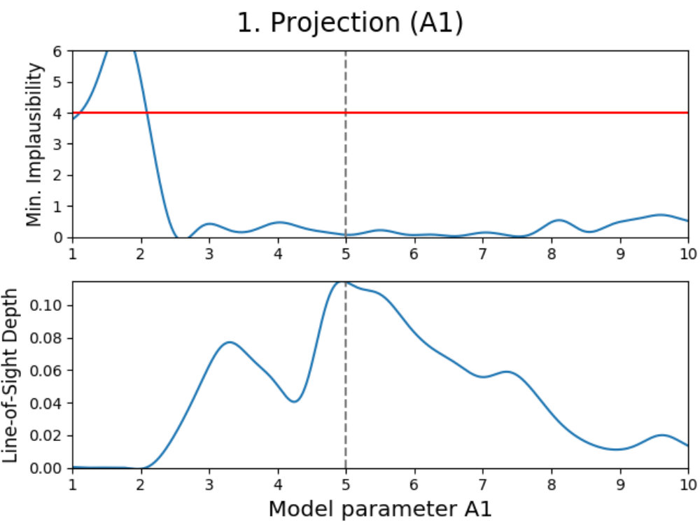 Figure 4
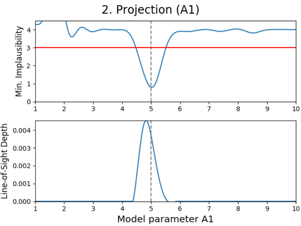 Figure 5
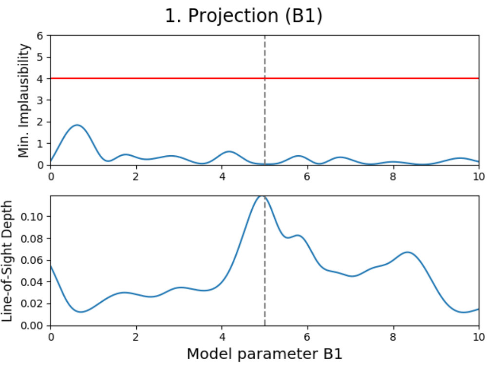 Figure 6
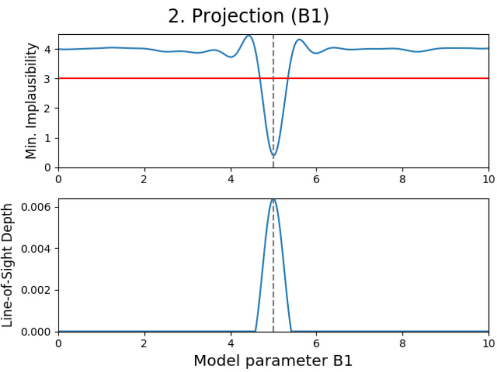 Figure 7
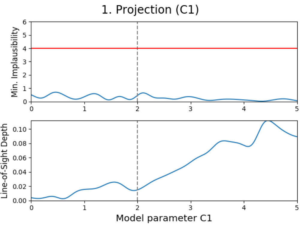 Figure 8
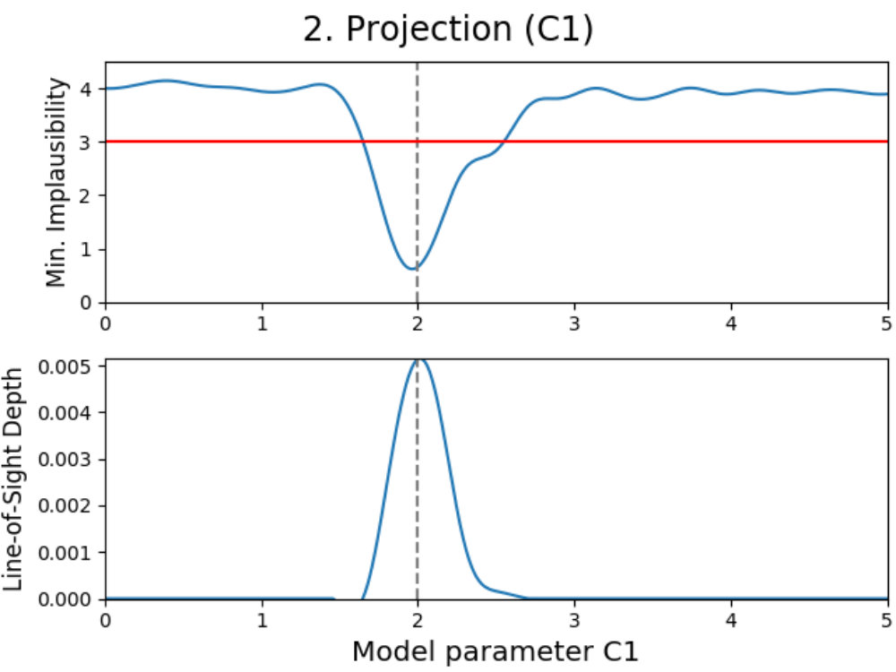 Figure 9
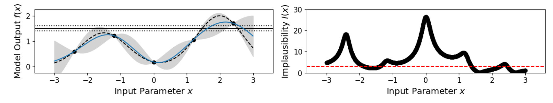 Figure 10
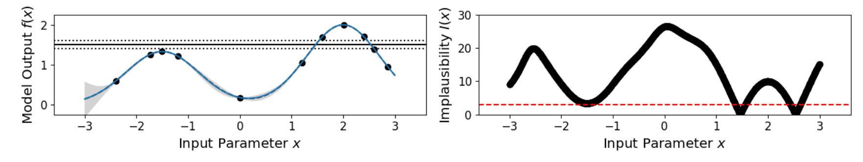 Figure 11
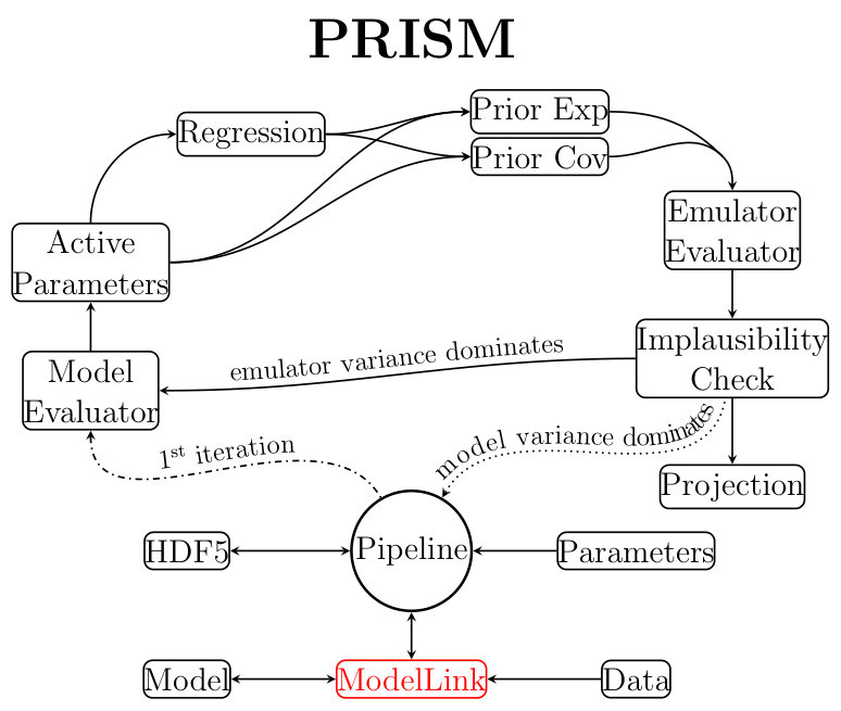 Figure 12
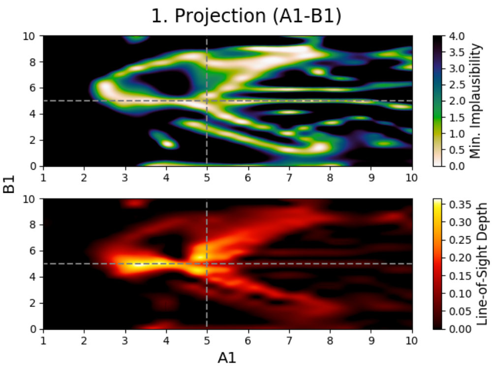 Figure 13
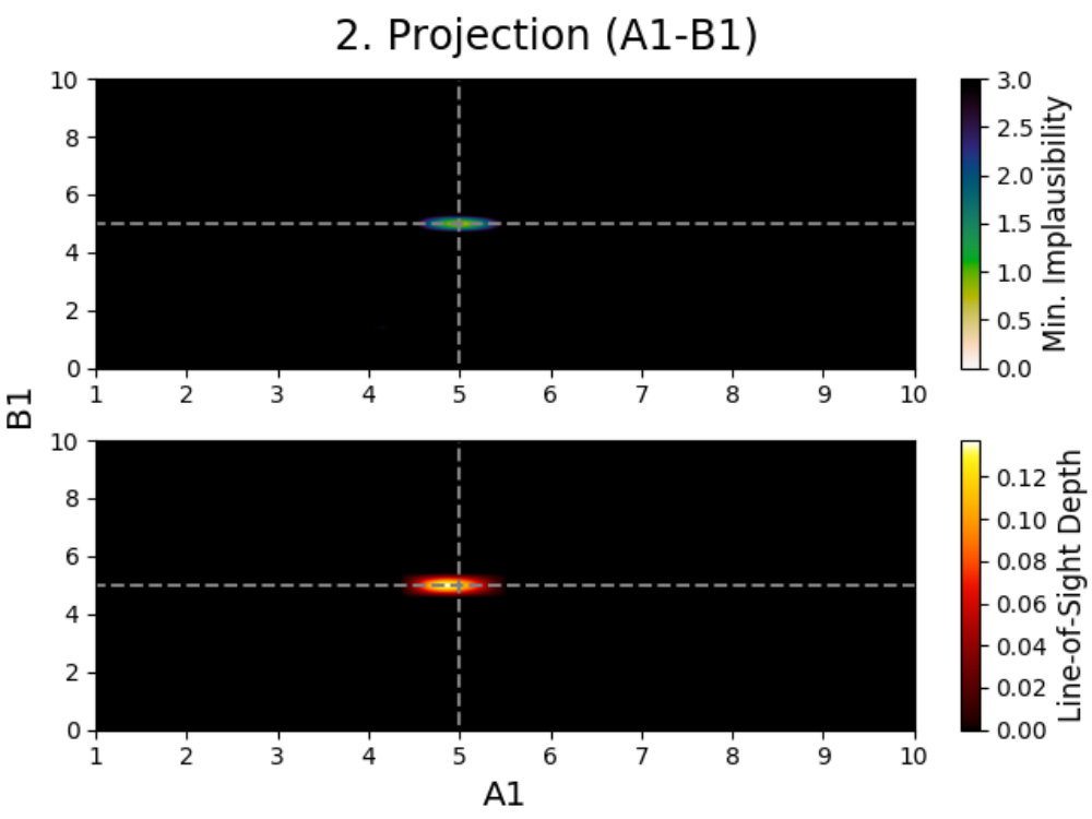 Figure 14
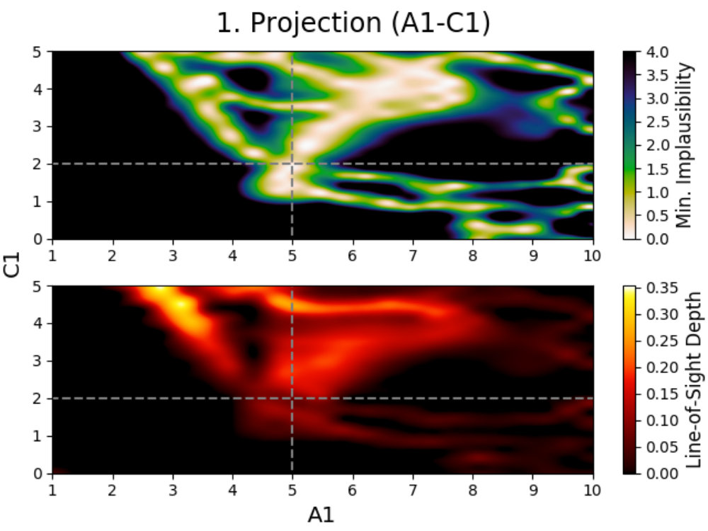 Figure 15
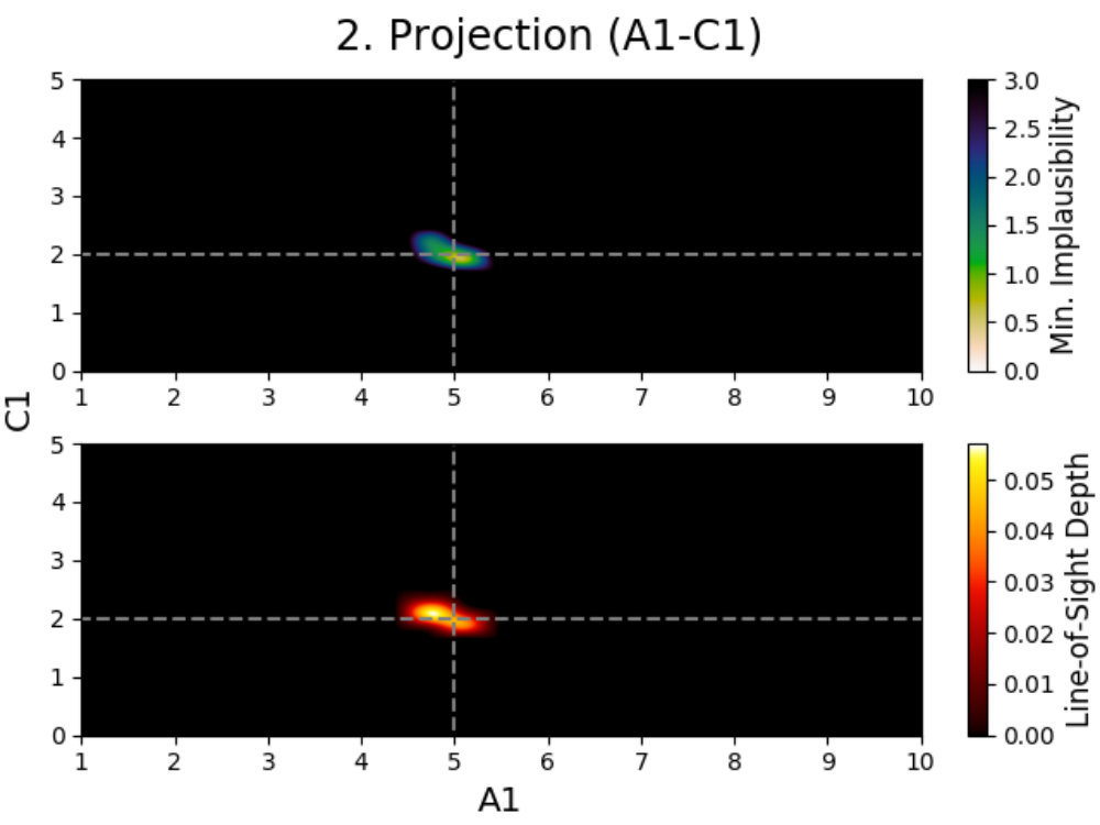 Figure 16
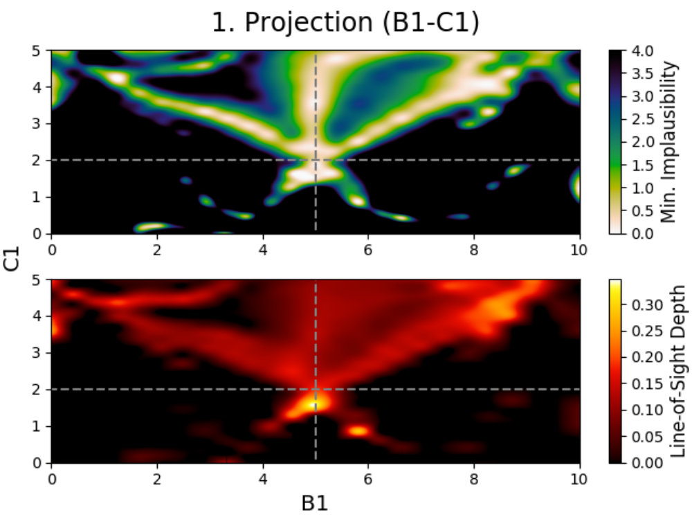 Figure 17
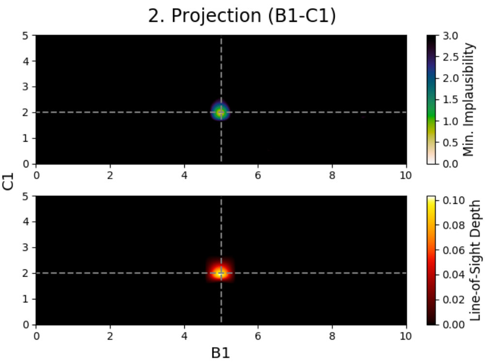 Figure 18
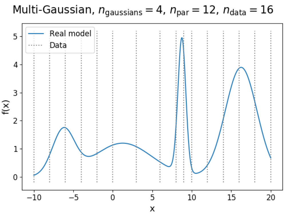 Figure 19
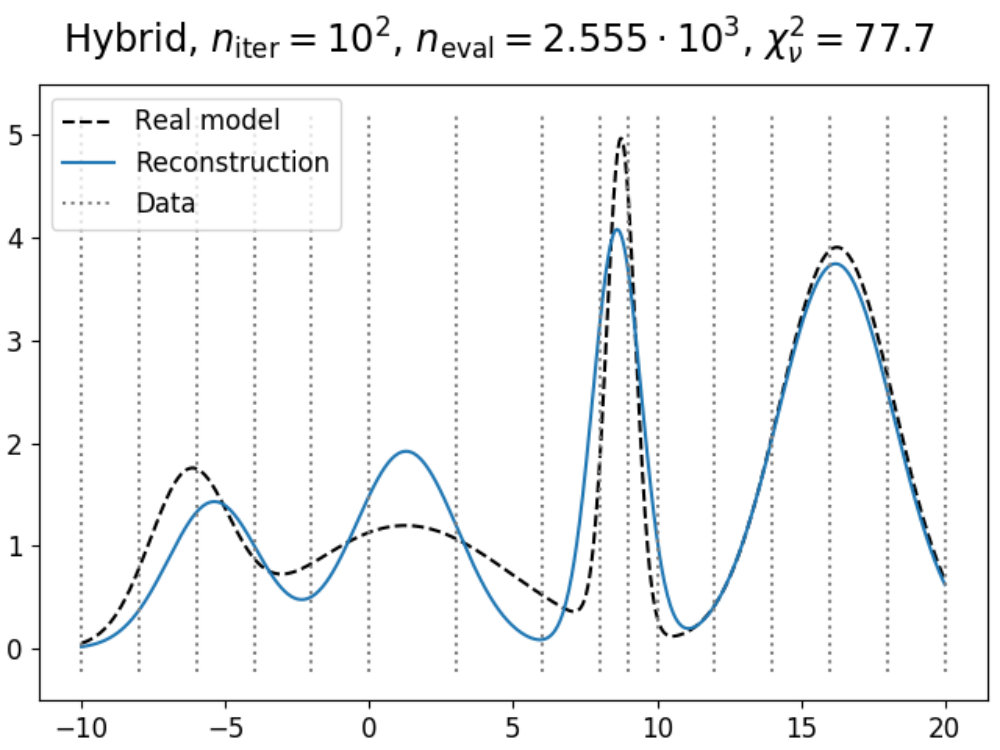 Figure 20
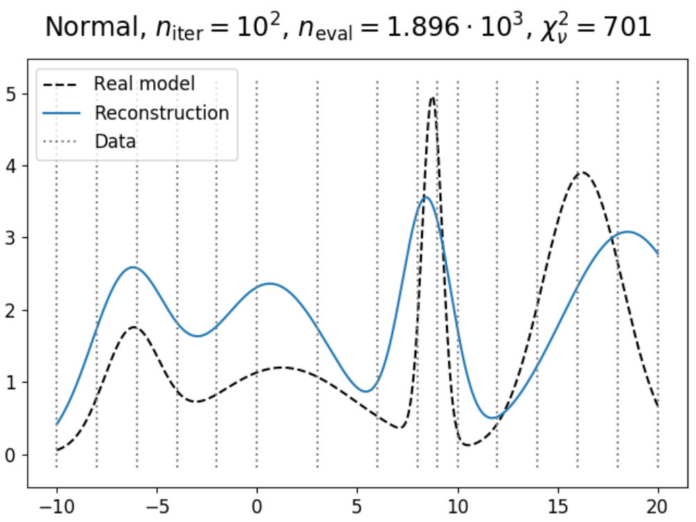 Figure 21
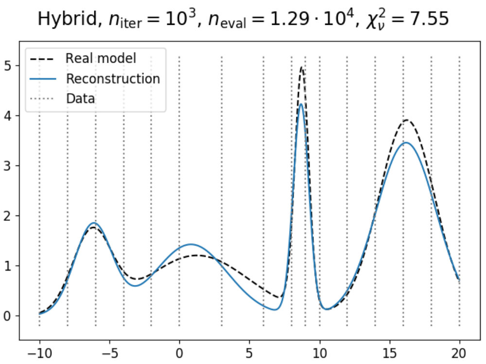 Figure 22
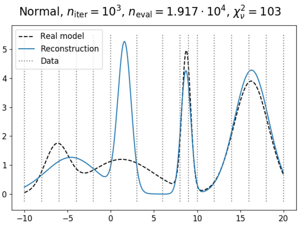 Figure 23
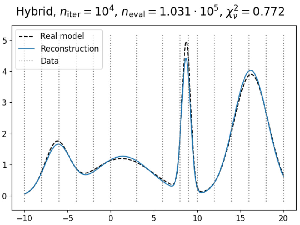 Figure 24
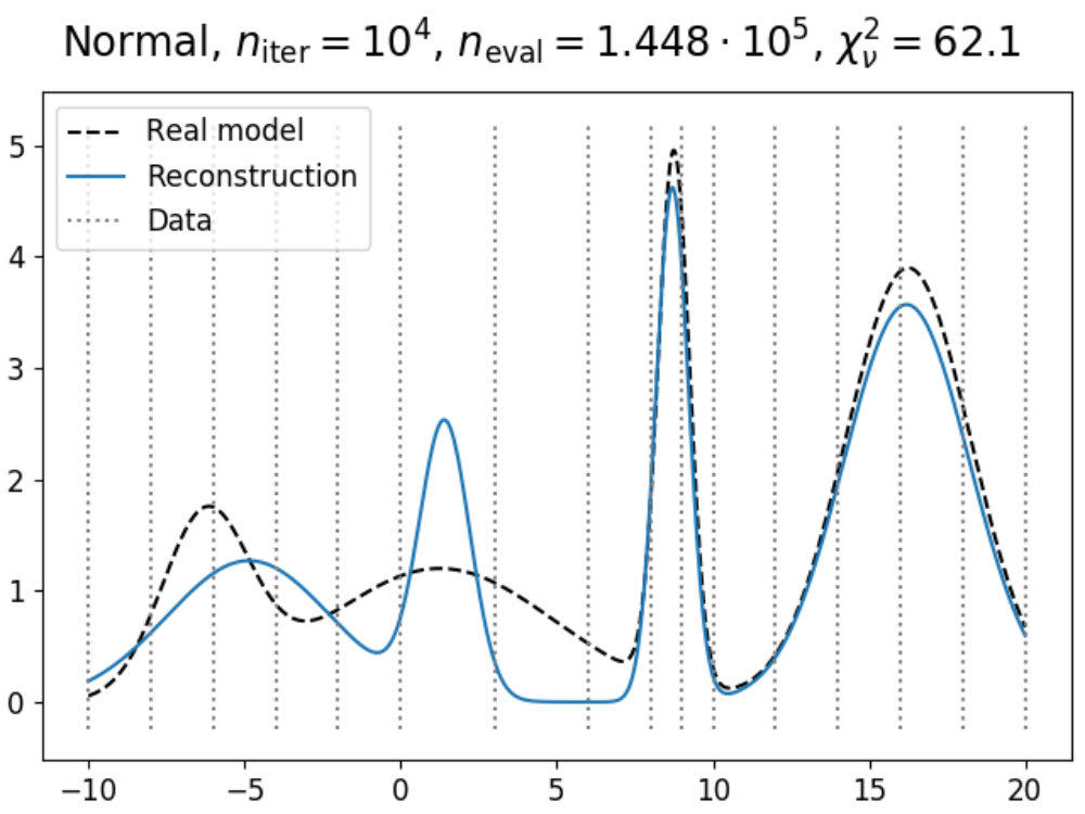 Figure 25
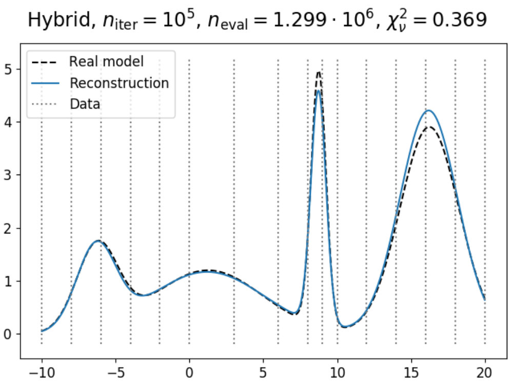 Figure 26
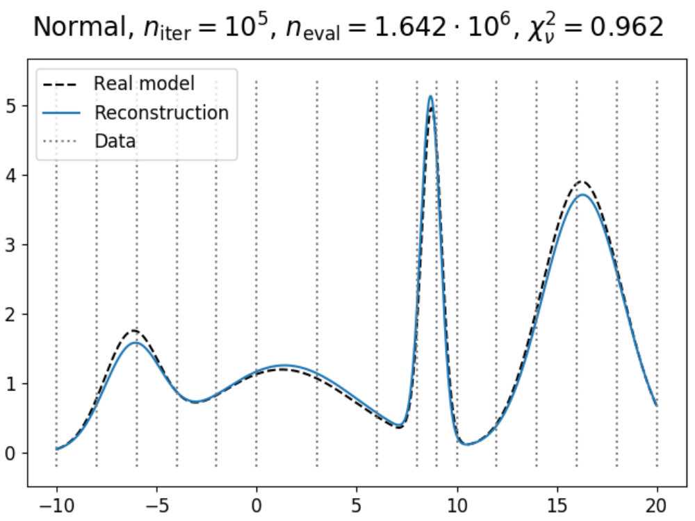 Figure 27
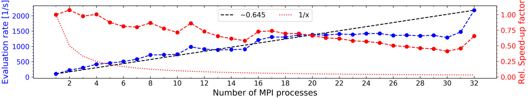 Figure 28
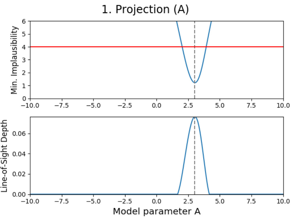 Figure 29
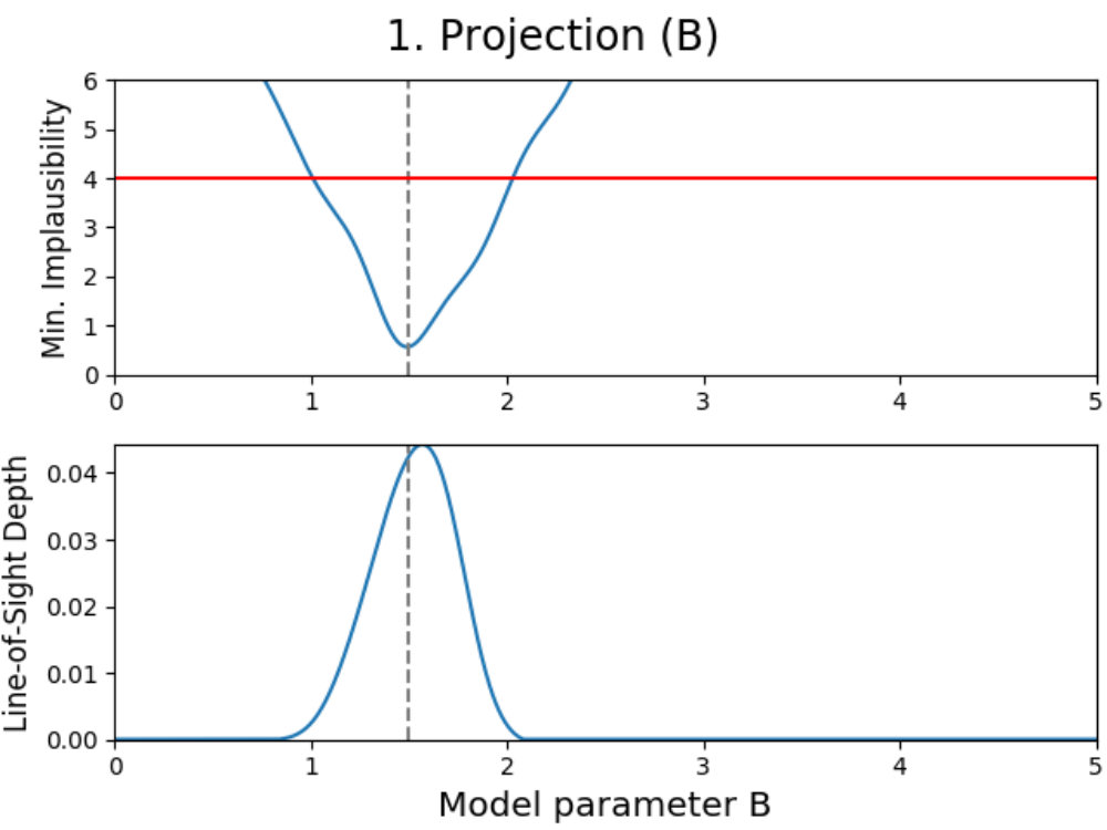 Figure 30
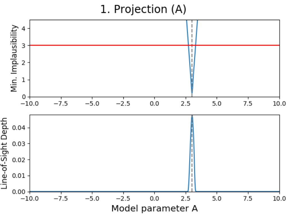 Figure 31
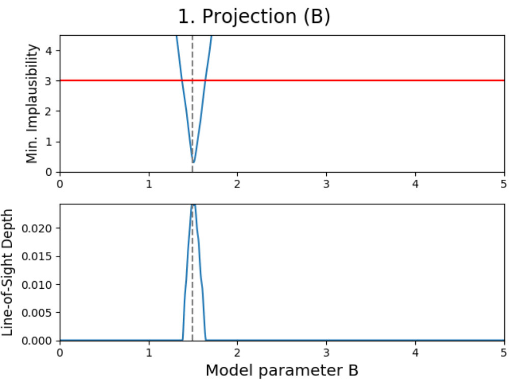 Figure 32
 Figure 33
 Figure 34
| \clineB3-102.5 | Hybrid | Normal | ||||||||
| \hlineB2.5 Name | Real | |||||||||
| \hlineB2.5 | ||||||||||
| \clineB2-102.5 | ||||||||||
| \clineB2-102.5 | ||||||||||
Peer Reviews
No public reviews on file for this paper yet. If you reviewed it on a platform where reviews are public (OpenReview, ICLR, NeurIPS, ICML), you can paste yours below so the community can read it here.
Code & Models
Videos
No videos yet. Explain this paper in a talk, walkthrough, or lecture? Add one.
Model dispersion with PRISM; an alternative to MCMC for rapid analysis of models
Centre for Astrophysics and Supercomputing, Swinburne University of Technology, PO Box 218, Hawthorn, VIC 3122, Australia
ARC Centre of Excellence for All Sky Astrophysics in 3 Dimensions (ASTRO 3D)
Centre for Astrophysics and Supercomputing, Swinburne University of Technology, PO Box 218, Hawthorn, VIC 3122, Australia
ARC Centre of Excellence for All Sky Astrophysics in 3 Dimensions (ASTRO 3D)
Centre for Astrophysics and Supercomputing, Swinburne University of Technology, PO Box 218, Hawthorn, VIC 3122, Australia
ARC Centre of Excellence for All Sky Astrophysics in 3 Dimensions (ASTRO 3D)
ARC Centre of Excellence for All Sky Astrophysics in 3 Dimensions (ASTRO 3D)
School of Physics, University of Melbourne, Parkville, VIC 3010, Australia
Centre for Astrophysics and Supercomputing, Swinburne University of Technology, PO Box 218, Hawthorn, VIC 3122, Australia
ARC Centre of Excellence for All Sky Astrophysics in 3 Dimensions (ASTRO 3D)
(Received 24/01/2019; Revised 29/04/2019; Accepted 03/05/2019)
Abstract
We have built Prism, a Probabilistic Regression Instrument for Simulating Models. Prism uses the Bayes linear approach and history matching to construct an approximation (‘emulator’) of any given model, by combining limited model evaluations with advanced regression techniques, covariances and probability calculations. It is designed to easily facilitate and enhance existing Markov chain Monte Carlo (MCMC) methods by restricting plausible regions and exploring parameter space efficiently. However, Prism can additionally be used as a standalone alternative to MCMC for model analysis, providing insight into the behavior of complex scientific models. With Prism, the time spent on evaluating a model is minimized, providing developers with an advanced model analysis for a fraction of the time required by more traditional methods.
This paper provides an overview of the different techniques and algorithms that are used within Prism. We demonstrate the advantage of using the Bayes linear approach over a full Bayesian analysis when analyzing complex models. Our results show how much information can be captured by Prism and how one can combine it with MCMC methods to significantly speed up calibration processes ( times faster). Prism is an open-source Python package that is available under the BSD 3-Clause License (BSD-3) at https://github.com/1313e/PRISM and hosted at https://prism-tool.readthedocs.io. Prism has also been reviewed by The Journal of Open Source Software (van der Velden, 2019).
methods: data analysis – methods: numerical
††journal: ApJS
1 Introduction
Rapid technological advancements allow for both computational resources and observational/experimental instruments to become better, faster and more precise with every passing year. This leads to an ever-increasing amount of scientific data being available and more research questions being raised. As a result, scientific models that attempt to address these questions are becoming more abundant, and are pushing the available resources to the limit as these models incorporate more complex science and more closely resemble reality.
However, as the number of available models increases, they also tend to become more distinct. This causes scientific phenomena to be described in multiple different ways. For example, there are many models in existence that attempt to describe the Galactic magnetic field (GMF, e.g., Sun et al. 2008; Jaffe et al. 2010; Pshirkov et al. 2011; Van Eck et al. 2011; Jansson & Farrar 2012a, b; Jaffe et al. 2013; Terral & Ferrière 2017; Unger & Farrar 2017) or study the formation of galaxies (e.g., Croton et al. 2016; Mutch et al. 2016; Lagos et al. 2018). Due to the complexity and diversity of such models, it is already a difficult task to compare them with each other (as demonstrated for GMF models by the IMAGINE pipeline, Steininger et al. 2018), but it can easily become just as difficult to keep track of their individual qualities. Therefore, a full analysis of every model would be required in order to recognize these qualities.
We commonly employ Markov chain Monte Carlo (MCMC) methods (Sivia & Skilling, 2012; Gelman et al., 2014) when performing this task. Monte Carlo methods are a class of algorithms that use the randomness of a system in order to solve problems, given that the problem is deterministic in principle. By repeatedly sampling randomly over the system, the idea of Monte Carlo methods is that with enough samples, the problem can be solved by a combination of these samples. If the problem can be parametrized, which is often the case with scientific models, this process can be sped up by adding one or several Markov chains to it. A Markov chain is (in this context) a sequence of evaluations where the outcome of every evaluation solely depends on the state the system was in right before it, creating a memoryless process. Doing so gives the class of MCMC methods.
When combined with a full Bayesian analysis, MCMC has the potential to create an accurate approximation of the posterior probability distribution function (PDF). This PDF can be used to identify regions of parameter space that compare well with the available data. Currently, there are many different MCMC methods available, like Metropolis-Hastings (Metropolis et al., 1953; Hastings, 1970); Gibbs (Geman & Geman, 1984); Hamiltonian/Hybrid Monte Carlo (Brooks et al., 2011; Betancourt, 2017); nested (Skilling, 2006); no-U-turn (Hoffman & Gelman, 2011); and affine invariant (Goodman & Weare, 2010) sampling to name but a few. Some of these are completely unique, while others are simply extensions of already existing methods to make them suitable for specific tasks.
However, as specialized as some MCMC methods are, they have a couple of drawbacks:
Random walk MCMC methods (methods based on the Metropolis-Hastings algorithm) tend to move around the equilibrium distribution of the model in relatively small steps or get stuck in local extrema, causing them to sample parts of parameter space that have been visited before. Not only does this make the process very slow, but it also causes the model to be reevaluated unnecessarily. Several MCMC methods, like Hamiltonian Monte Carlo, try to circumvent this by not using a random walk algorithm, but instead use the gradient field of the desired distribution. This however does require one to have additional knowledge about the model and that the gradient field exists, which might be difficult to obtain due to the number of degrees-of-freedom involved; 2. 2.
Given the discontinuous and irregular natures some models tend to have, MCMC methods can completely fail to converge due to irregularities in the probability distribution. This also increases the difficulty of obtaining a description of the gradient field, since it is not defined everywhere; 3. 3.
The rate at which an MCMC method converges depends on the initial number of samples and their locations. Not using enough may cause it to never converge, while using too many will make the process move forward very slowly.
Given the reasons above, it may not look appealing to some to perform an extensive model analysis. However, we believe that analyzing a model does not necessarily require the full posterior PDF to be accurately known. Instead, the converging process towards this PDF provides insight on the workings of a model. Therefore, we propose to use a combination of the Bayes linear approach and the emulation technique with history matching, which can be seen as special cases of Bayesian statistics.
The emulation technique can be used to create an emulator, which is an approximate system of mainly polynomial functions and Gaussian processes based on limited knowledge about the model. Using the Bayes linear approach and history matching, an emulator can quickly make predictions on the expected relevance (‘implausibility’) of all parts in model parameter space, taking into account the variance that is introduced by doing so. By imposing cutoffs on this relevance, parts of parameter space can be excluded, defining a smaller parameter space over which an improved emulator can be defined. Performing this process iteratively allows one to quickly reduce the size of relevant parameter space while being provided with several snapshots of the convergence process, giving insight on the model’s behavior.
These techniques have been applied to various systems several times in the past (either together or separately), including the study of whales (Raftery et al., 1995), oil reservoirs (Craig et al., 1996, 1997), galaxy formation (Bower et al., 2010; Vernon et al., 2010, 2014; Rodrigues et al., 2017), disease studies (Andrianakis et al., 2015, 2016, 2017), biological systems (Vernon et al., 2018) and simply described in general (Sacks et al., 1989; Currin et al., 1991; Oakley & O’Hagan, 2002; O’Hagan, 2006). Many of these works show how much information can be extracted from an emulator, and the advantages the combination of the Bayes linear approach, emulation technique and history matching has over using a full Bayesian analysis. However, the algorithms used are often focused on a specific application and are typically not publicly available.
In this work, we introduce Prism, a Probabilistic Regression Instrument for Simulating Models. Prism is a publicly available framework that uses the Bayes linear approach to combine the power of emulation with the process of history matching. Although this has been done before (e.g., Bower et al. 2010; Vernon et al. 2010, 2014; Rodrigues et al. 2017; Vernon et al. 2018), Prism is unique in that it is not built for a specific application. Instead, Prism provides a universal, versatile framework in which both simple and sophisticated models can be analyzed with minimal effort. Additionally, its implementation is highly modular, allowing for extensions to be added easily.
In 2, we describe the Bayes linear approach, emulation technique and history matching, which are the main methods behind analyzing models with Prism. Then, using this knowledge, we give an overview of the Prism framework in 3 and its various components. We show in 4 what Prism can do when combined with and compared to normal MCMC methods. Finally, we give a short introduction to the larger applications that Prism will be used for in 5.
2 Model analysis
In this section, we describe the various different techniques that are used in Prism, including a discussion on variances, the Bayes linear approach and the emulation technique, history matching and implausibility measures. Note that this section is meant for those seeking a general understanding of the used methodology. See Vernon et al. (2010) for further details and justification. For those looking for a description of Prism itself, we refer to 3.
2.1 Uncertainty analysis
When evaluating a model, it is required to have knowledge of all the individual components that influence the outcome of the model before performing the actual evaluation. This allows one to interpret the meanings behind the constructed model realization, determine its accuracy by comparing it to the physical system one is describing and study its behavior. Due to a variety of reasons, these components each contribute to how certain (or uncertain) one is that the output given by the model is correct given the observational data. When performing an analysis on a scientific model, it is important to know what all the individual contributions to the uncertainty are. Below, we give an overview of the most common uncertainty contributions, describe the underlying process and how they are treated in this work.
Observational uncertainties
In order to explain the Universe, one attempts to make a connection between observations and modelling. However, observational instruments are not perfect, giving rise to uncertainties in the true value of the observed data. Additionally, measurements are often obtained by performing conversions/integrations on the observations, increasing the uncertainty. In this work, the uncertainties described above are collected into one term called the observational variance, which for a single data point is denoted by .
Model output uncertainties
The output of a model is usually determined by individual contributions from a large number of deterministic functions, which combined can be seen as a single deterministic computer function. Because evaluating this single function is often very expensive, it is appropriate to say that the output of the function is unknown for almost all combinations of input parameter values. In this work, we attempt to solve this problem by creating a statistical representation of this function by constructing something called an emulator (see 2.3). While the model discrepancy variance discussed below gives the contribution to the overall uncertainty of the known model realizations, the emulator variance describes the uncertainty of the unknown realizations.
Knowledge uncertainties
Since the observational data that we have at our disposal is exhaustive, the possibility exists that we have overlooked a certain dynamic, mechanic or phenomenon that is important for the model. Additionally, limited computational resources often force us to use approximations of the involved physics or use other models, inevitably introducing uncertainties to the problem. Although very small, these are all contributions to the knowledge uncertainty of the model, causing a discrepancy between reality and the model. This so-called model discrepancy variance (Craig et al., 1996, 1997; Kennedy & O’Hagan, 2001; Vernon et al., 2010) is usually the most challenging of all uncertainties and it is very important to not underestimate its contribution to the total variance involved. Given its importance, we give a more detailed description of this in 3.4, describing how Prism treats different variances.
2.2 Bayes linear approach
As discussed in 1, performing a full Bayesian analysis on a complex model can be quite complicated. In order to undertake such a Bayesian analysis, one uses Bayes’ equation given as:
[TABLE]
where is the model (realization), the comparison data and the remaining background information. Bayes’ equation gives one the probability that a given model realization can explain the comparison data , taking into account the background information .
Although this gives one an absolute answer, it is required for the user to parametrize everything about the model in order to quantify its prior, . This includes that one knows all uncertainties that are related to the model in question. Not only that, but it is also required to specify a meaningful likelihood, which is often very difficult to do properly, as this requires realistic assumptions and robustness (slight changes in the likelihood form should not massively alter its outcome). And, finally, the same applies for the comparison data, since it is required to know the evidence value, , as well when dealing with model comparisons. It is therefore necessary to have full knowledge about the model and the data one wants to use, which may be hard or even impossible to obtain.
Another complication here is how one finds the parameter set that can explain the comparison data the best. As mentioned before, we commonly employ MCMC methods to perform this task. Although MCMC can narrow down parameter space where one can find the exact model realization that can explain the comparison data the best, it requires many evaluations of the model in order to get there. When dealing with complex models, one usually does not want to unnecessarily evaluate the computationally expensive model. It is therefore not seen as ideal to evaluate the model in parts of parameter space where the probability of finding that exact parameter set, is very low. This does however happen fairly often due to the nature of MCMC, which tries to find its path through parameter space by sampling in random directions and accepting new samples with certain probabilities (which is commonly known as Metropolis-Hastings sampling, Metropolis et al. 1953; Hastings 1970).
There is a more appropriate method to analyze a complex scientific model. Instead of using full Bayesian analysis and MCMC methods, we use the Bayes linear approach (Goldstein, 1999; Goldstein & Wilkinson, 2000; Goldstein & Wooff, 2007). The difference between the Bayes linear approach and a full Bayesian analysis, is that the Bayes linear approach uses expectations as its primary output instead of probabilities. The advantage of this is that the Bayes linear approach does not require the full joint specification of an appropriate probabilistic model for the prior and all associated data points (which is required for determining probabilities), allowing one to use it even when not all details are known. This makes the Bayes linear approach much simpler in terms of belief and analysis, since it is based on only the mean/expectation, variance and covariance specifications, for which we follow the definitions by De Finetti (1974, 1975). The two main equations of the Bayes linear approach are the updating equations for the expectations and variances of a vector (the model realization), given a vector (the comparison data):
[TABLE]
where and are known as the adjusted expectation and adjusted variance of given (Goldstein, 1999; Goldstein & Wooff, 2007).
The equation for the adjusted expectation is fairly similar in meaning to Bayes’ equation. In the Bayes linear approach, the expectation of the model realization is the equivalent of the probability that is correct in full Bayesian analysis. In particular, if one would use a full Gaussian specification for all of the relevant quantities, one would end up with similar updating formulas. An overview of the Bayes linear approach is given in Goldstein (1999), and we direct readers to Goldstein & Wooff (2007) for a detailed description of it.
There are two general reasons for why one may choose the Bayes linear approach over a full Bayesian analysis. We discussed earlier that performing a full Bayesian analysis can take a significant amount of time, and may not be possible due to constraints on knowledge and computational resources. In this scenario, one could view the Bayes linear approach as a special case of full Bayesian analysis. The Bayes linear approach is simplified compared to a full Bayesian analysis, since we only require the expectations, variances and covariances of all random quantities that are involved in the problem. Therefore, instead of carrying out a full posterior calculation using Bayes’ equation given in 1, we carry out a Bayes linear update by using 2 and 3. The adjusted expectation value of given () can be seen as the best linear fit for , given the elements in the data , with the adjusted variance value being the minimized squared error. This best linear fit depends solely on the collection of functions of the elements in the data , which can be chosen to be whatever we like it to be. If we would choose all functions that are possible in the data (up to infinite order polynomials), we are effectively recreating the full Bayesian analysis.
The second, more fundamental reason comes from the meaning of a full Bayesian analysis. A full Bayesian analysis has a lot of value, since it allows others to include their own expertise and knowledge in the analysis of their model. However, at some point, models become so complex and sophisticated, that it becomes hard to make expert judgments on the prior specifications of the model, which are required for doing a full Bayesian analysis. The Bayes linear approach however, does not require the specifications of any prior distribution (which can be very complex), but instead requires the simpler prior expectations and (co)variances of a model realization, which can still be used for including expert prior knowledge. For a more detailed overview of these two reasons, see Goldstein (2006).
The benefit of the Bayes linear approach combined with the emulation technique and history matching is that it does not require a high number of model evaluations in order to say something useful about the model. For example, one can usually already exclude certain parts of parameter space based on minimal knowledge of the model, as long as taking into account all related variances still does not make it likely that this part is important. Therefore, using the Bayes linear approach in this way allows one to decrease the part of parameter space that is considered important and only evaluate the model there, by only having a limited amount of knowledge. This is a big advantage over using a traditional full Bayesian analysis with MCMC methods, since MCMC will not have this knowledge (due to its Markov chain nature) and therefore can potentially have a large burn-in phase.
Another benefit of the Bayes linear approach (when combined with the emulation technique and history matching) that can be crucial to model analysis, is its ability to accept additional constraints while already analyzing a model. When performing a full Bayesian analysis, it is required that it already contains all constraints (given by data, previously acquired results, etc.) that one wants to put on the model. If one would attempt to introduce additional constraints during a full Bayesian analysis, it could potentially corrupt the results or confuse the process. However, since the expectation value of the model realization () is important rather than the model realization itself, additional comparison data can be easily added to the analysis at a later stage, without requiring the model to be reevaluated at all previously evaluated samples. This allows for one to update/improve their analysis of a model when new data becomes available or to only incrementally add data constraints in order to minimize the amount of time spent on evaluating.
2.3 Emulation technique
When analyzing a model, it is usually desirable to cover its full parameter space. This would allow one to study the dependencies between all parameters and their behaviors in general. However, this approach rapidly becomes unfeasible when one increases the number of model parameters. If one does not make any assumptions about the dependencies between model parameters, then the easiest way of model exploration is achieved by direct sampling, which means that every single combination of model parameters needs to be checked. In other words, choosing different values for every of the model parameters, will yield different combinations. Anything more than model parameters will already give a very large number of model realizations to be evaluated, while the density of evaluated samples in parameter space is extremely low. In order to avoid this, a different approach is required.
We propose to use the technique of emulation, by constructing a so-called emulator system for every output of a given model. An emulator system can be described as a stochastic belief specification for a deterministic function, which has been successfully applied to various systems several times in the past (e.g., Sacks et al. 1989; Currin et al. 1991; Craig et al. 1996, 1997; Oakley & O’Hagan 2002; O’Hagan 2006; Bower et al. 2010; Vernon et al. 2010, 2014, 2018). Unlike a model, an emulator system can be evaluated very quickly, allowing one to explore its parameter space in a more efficient way. Knowing this, we substitute a collection of emulator systems (called an emulator) for the model evaluations, while taking into account the additional variances that are introduced in doing so.
Following the form used in Vernon et al. (2010), an emulator system is constructed in the following way. Suppose that for a vector of input parameters , the output of a model is given by the function . If the output of this model would have no variance, then we can say that (output of ) is given by a function , which has the form
[TABLE]
where are unknown scalars/coefficients, are known deterministic functions of and is known as the regression term.
Realistically speaking, we are uncertain if follows the above description for every , as we have not evaluated everywhere and thus we do not know all of its corresponding outputs. Therefore, it is required to add a second term to that describes this uncertainty, which gives
[TABLE]
with a weakly stochastic process with constant variance and uncorrelated with the regression term . The regression term describes the general behavior of the function, while represents the local variations from this behavior near .
When dealing with high dimensional parameter spaces, it is not unusual to find that a subset of the model parameters can explain a significant part of the variance in the model output. Therefore, we introduce the so-called active parameters, , which is a subset of and varies with . However, due to the introduction of active parameters, one final term needs to be added to , changing it to
[TABLE]
where is the variance in caused by the passive parameters.
When using the Bayes linear approach, the emulator system requires the definition of the prior expectation and the prior (co)variance of all three terms in 6. Commonly, localized deviations in a function are assumed to be of Gaussian form, which has a covariance that is defined as
[TABLE]
with and being the Gaussian variance and correlation length, respectively. The Gaussian correlation length is defined as the maximum distance between two values of a specific model parameter within which the Gaussian contribution to the correlation between the values is still significant.
Here, is called the Gaussian term and has an expectation of zero. The other variation term, the so-called passive term, , describes the variance that is caused by passive parameters and therefore has no expectation value and a constant variance :
[TABLE]
with the Kronecker delta of and .
We can now use the emulator system to evaluate and calculate the expectation and variance values of the function for any input , and the covariance between values of for any pair of inputs . From 6, we get that the prior expectation is given by
[TABLE]
and that the prior covariance is given by
[TABLE]
where all cross-covariances are equal to zero (as all three terms are uncorrelated). Here the first term is the covariance of the regression term, which can be derived using the relation :
[TABLE]
This is all that is required for the Bayes linear approach in order to update our beliefs in terms of expectation and variances about the model output at an unevaluated input , given a set of known model realizations. This process is described below.
Suppose that we have evaluated the model for different input parameter sets. Then we can write the individual inputs as with , where each represents the vector of parameter values in parameter space for the evaluation. Using the same notation, gives the vector of active parameter values for the evaluation. We define the vector of model outputs for output of known model realizations as . If we now replace the vector in the Bayes linear approach update equation of the expectation value (2) with the model output and vector with , we obtain the adjusted expectation for a given emulator system :
[TABLE]
where is the vector of covariances between the new and known points, and is the matrix of covariances between known points with elements .
Similarly, the adjusted variance can be found by combining 9 and 10 with 3:
[TABLE]
The adjusted expectation, , and adjusted variance, , represent our updated beliefs about the output of the model function for model parameter set , given a set of model evaluations with output . These adjusted values are used in the implausibility measures for the process of history matching, which are described in 2.4. Note that the adjusted values for any known model evaluation are equal to and . For further discussion, we point interested readers to Vernon et al. (2010, 2018).
From 12 and 13, it is clear that the regression term and the Gaussian term are strongly connected to each other: increasing the variance that the regression term can explain will decrease the remaining variance that is described by the Gaussian term and vice verse. Since the regression term is much more complicated than the Gaussian term, one could argue here whether it is preferable to put a lot of time, effort and resources in constructing the regression term for every emulator system, while one can also place more weight on the Gaussian term. By default, Prism aims to explain as much variance as possible with the regression term, but this balance is provided as a user-chosen parameter. The reasons why we prefer putting a lot of emphasis on the regression term are:
We aim to make Prism suited for analyzing any given model, but in particular those that are highly complex. Such models often have strong physical interpretations and interactions driving them, influencing the results that the model gives. The embedded physical laws are often reasonably well-behaved and therefore usually come in the form of polynomial functions, making it only natural to express them in the same way through the regression term; 2. 2.
Studying the behavior of the model according to the emulator system, is much easier to do when one is given the polynomial terms and their expected coefficients. This allows the user to check whether the emulator system is consistent with expectation, while also allowing for new physical interactions to be discovered; 3. 3.
The more information is contained within the regression term, the less information remains for the Gaussian term. This makes it easier to compare emulator systems with each other, while also allowing one to remove the calculation of the Gaussian term if the remaining (Gaussian) variance drops below a certain threshold; 4. 4.
And most importantly, the Gaussian term, , is an approximation in itself (of Gaussian form) and therefore might have trouble explaining the smoothness of a complex model on both large and small scales simultaneously. A Gaussian correlation (or any other correlation form) makes certain assumptions about the behavior of the model. If the model does not follow these assumptions, a correlation can have trouble coming up with a good fit. Therefore, the Gaussian term is mainly used for explaining local behavior, whereas the regression term captures the global behavior.
In summary, for each model output, one is required to:
- •
have a collection of known model realizations ;
- •
identify the set of active parameters ;
- •
select the polynomial regression terms ;
- •
determine the coefficients of these terms ;
- •
obtain the residual variance from the regression term;
- •
and, if required, calculate the covariance of the polynomial coefficients .
Then, we can use 12 and 13 to update our beliefs on the model output function , by obtaining the adjusted expectation and covariance values for any given parameter set . Afterward, we have to carry out a diagnostic analysis on the emulator, or we can alternatively decide to study the properties and behavior of the emulator by making a projection first (see 4.2). This diagnostic analyzing of the emulator is called history matching and is explained below.
2.4 History matching
The idea behind Prism is to provide the user with the collection of parameter sets that gives an acceptable match to the observations when evaluated in . This collection contains the best parameter set as well as parameter sets that yield acceptable matches and can be used for studying the properties of the emulated model. The process of obtaining this collection is usually referred to as history matching. This terminology is common in various different fields (Raftery et al., 1995; Craig et al., 1996, 1997), although one rarely tries to find all matches instead of just a few. To give the user more flexibility and more information, we think it is better to try to find as many matches as possible.
The process of history matching can be compared to model calibration (discussed in more detail in Vernon et al. 2010, 2018), where we assume that there is a single true but unknown parameter set and our goal is to make probabilistic statements about based on a prior specification, the collection of model evaluations and the observed history (Kennedy & O’Hagan, 2001; Goldstein & Rougier, 2006). Although history matching and model calibration look alike and are certainly related, they are very different in terms of approach. Whereas model calibration gives one a posterior PDF of parameter space that can be used to evaluate various parameter sets, history matching can conclude that no best parameter set exists even if it should. If this is the case, this might be an indication that there are some serious issues with the model, while model calibration can have trouble coming to the same conclusion. Because of this, we think that history matching is very important for analyzing complex models.
The way we approach history matching is by evaluating so-called implausibility measures (Craig et al., 1996, 1997), for which we use the same form as in Vernon et al. (2010). An implausibility measure is a function that is defined over parameter space which gives a measure of our tolerance of finding a match between the model and the modelled system. When the implausibility measure is high, it suggests that such a match would exceed our stated tolerance limits, and that we therefore should not consider the corresponding parameter set to be part of . If we again consider to be a single model output, then we would like to know for a given parameter set whether the output is within tolerance limits when compared to the system’s true value . In order to do this, we would have to evaluate the standardized distance given as
[TABLE]
In reality, we do not know and instead have to use its observed value , which has its own measurement error and converts the standardized distance to
[TABLE]
However, for most parameter sets , we are not able to evaluate the model and obtain . Therefore, we have to use the emulated value and compare this with . This defines the implausibility measure as
[TABLE]
Using 14 and taking into account that the data, model and emulator system have a variance, we obtain the implausibility measure for the emulator system:
[TABLE]
with the adjusted emulator expectation (12), the adjusted emulator variance (13), the model discrepancy variance and the observational variance.
When, for a given parameter set , the corresponding implausibility value is large, it suggests that it would be unlikely that we would view the match between the model output and the comparison data as acceptable, if we would evaluate the model at this parameter set. Therefore, whenever this happens, we can say that any parameter set for which the implausibility value is large, should not be considered part of the potential parameter sets in the collection . By imposing certain maximum values for the implausibility measure, we can ensure that only those parameter sets that give low implausibility values are not discarded. Seeing that the distribution of the function is both unimodal (the two terms in 12 are independent of each other and ) and continuous (the emulator system solely contains deterministic functions) for a fixed parameter set , we can use the -rule given by Pukelsheim (1994). This rule implies that for any continuous, unimodal distribution, of its probability must lie within (), which even applies for asymmetric, skewed, tailed or heavily varying distributions. Values higher than would usually mean that the proposed parameter set should be discarded, but Prism allows the user full control over this.
To illustrate how the theory above can be applied to a model, we have used the emulation method on a simple double Gaussian model, given in Fig. 1. Here, we have made an emulator of a model defined as
[TABLE]
which are two Gaussians with different mean and amplitude, and a standard deviation chosen such that . On the left in 1a, the real model function is shown in dashed black (which usually is not known, but displayed for convenience), which has been evaluated a total of times as indicated by the black dots. Using these evaluations, we can construct an emulator using 12 and 13, where the adjusted expectation value is given by the solid (light blue) line and its confidence interval by the shaded area, where here is defined as .
Now suppose that we also have a comparison data point, given as the black horizontal line with its confidence interval. Using the constructed emulator, we can determine for what values of we expect a model realization that might be within our stated tolerance of , whose results are shown on the right in 1a. From the plotted implausibility values, we can see that there are small parts of parameter space that are likely to yield such model realizations and therefore require further analysis. By evaluating the model more times in the plausible region and defining a new emulator using these evaluations, we obtain the plots in 1b. We can now see that the emulator has been greatly improved in the regions of parameter space that were still interesting, and that the implausibility values are only low enough around and , which is as expected.
Obviously, the example given in Fig. 1 is highly simplified and does not even require emulation to solve. For more complex models with more parameters and outputs, the problem quickly becomes too complicated to cover by a single emulator system. In Prism, every model output has its own implausibility measure defined, since every emulator system is vastly different from another. However, all emulator systems (the emulator) share the same parameter space and a parameter set must give acceptable results in every emulator system to be considered part of the collection . Therefore, it is required that we combine the various different implausibility measures together in order to know which parts of parameter space are definitely not contained within . By maximizing over , one obtains the highest implausibility value that is reached for all these outputs. This so-called maximum implausibility measure is given by
[TABLE]
This measure can be used to rate the emulated outputs in terms of how well they compare to the comparison data .
However, early on in the emulation process, the emulator systems are still fairly inaccurate due to a low density of model evaluation samples. This causes these emulator systems to have a high probability of excluding a part of parameter space that should not be excluded or at least currently still contains acceptable choices for . Therefore, one should not select the highest implausibility value, but the second (or third) highest implausibility value as a safety measure early on. This is then given by
[TABLE]
with () being the highest (second-highest) implausibility value and ‘’ meaning ‘except/without’. Generalizing the functions above, gives the function for the so-called implausibility cut-off as
[TABLE]
History matching is an iterative process, in which parts of parameter space are removed based on the implausibility values of evaluated parameter sets, which in turn leads to a smaller parameter space to evaluate the model in. This process is known as refocusing (described in Vernon et al. 2010), and Prism uses this process to shrink down parameter space with every step. At each iteration , the algorithm can be summarized in the following way:
A Latin-Hypercube design (McKay et al., 1979) of parameter sets is created over the current plausible region , which is based on all preceding implausibility measures (or covers full parameter space if no previous iterations exist); 2. 2.
Each parameter set in this Latin-Hypercube design is evaluated in the model; 3. 3.
The active parameters are determined for every model output (see 3.3); 4. 4.
The corresponding model outputs are used to construct a more accurate emulator which is solely defined over the current plausible region ; 5. 5.
The implausibility measures are then recalculated over by using the new emulator systems; 6. 6.
Cut-offs are imposed on the implausibility measures, which defines a new and smaller plausible region which should satisfy ; 7. 7.
Depending on the user, repeat step 1 to 6 unless a certain condition is met; 8. 8.
Prism stops improving the emulator and gives back its final results.
We have multiple different reasons to believe that every iteration will decrease the part of parameter space that is still considered plausible:
Increasing the density of model evaluations in parameter space gives the emulator systems more information and therefore increases their accuracy. However, since the emulator systems are not required to have a high accuracy in order to exclude parts of parameter space, it is important to only gradually increase the density to allow for higher evaluation rates. The algorithm above ensures that this happens; 2. 2.
Reducing the plausible region of parameter space might make it easier for the emulator systems to emulate the model output and therefore make the function smoother; 3. 3.
All parameters that were not considered active in earlier iterations due to them not accounting for much of the variance, may become active in the current one, allowing more variance to be captured by the emulator systems.
The use of continued refocusing is very useful, but it also has its complications. For example, the only way of knowing if a parameter set is contained within the plausible region, is by calculating the implausibility values for all its model outputs and then using 16 to see if it satisfies all imposed implausibility cut-offs. Although evaluating a single parameter set can be done very quickly, obtaining a reasonably sized Latin-Hypercube design for step 1 in the algorithm requires the evaluation of thousands, tens of thousands and maybe even hundreds of thousands of parameter sets. This means that Prism must be fast and efficient in evaluating model parameter sets. A full detailed description of Prism is given in 3.
3 PRISM pipeline
3.1 Structure
The overall structure of Prism (as of version ) can be seen in Fig. 2 and will be discussed below. The Pipeline object plays a key-role in the Prism framework as it governs all other objects and orchestrates their communications and method calls. It also performs the process of history matching and refocusing (as explained in 2.4). It is linked to the model by a user-written ModelLink object (see 3.2), allowing the Pipeline object to extract all necessary model information and call the model. In order to ensure flexibility and clarity, the Prism framework writes all of its data to one or several HDF5-files111https://portal.hdfgroup.org/display/HDF5/HDF5 using h5py (Collette, 2013), as well as NumPy (Oliphant, 2006).
The analysis of a provided model and the construction of the emulator systems for every output value, start and end with the Pipeline object. When a new emulator is requested, the Pipeline object creates a large Latin-Hypercube design (McKay et al., 1979) of model evaluation samples to get the construction of the first iteration of the emulator systems started. To ensure that the maximum amount of information can be obtained from evaluating these samples, we have written a custom Latin-Hypercube sampling code based on the work by Joseph & Hung (2008). This produces Latin-Hypercube designs that attempt to satisfy both the maximin criterion (Johnson et al., 1990; Morris & Mitchell, 1995) as well as the correlation criterion (Iman & Conover, 1982; Owen, 1994; Tang, 1998). This code is customizable through Prism and publicly available in the e13Tools222https://github.com/1313e/e13Tools Python package.
This Latin-Hypercube design is then given to the Model Evaluator, which through the provided ModelLink object evaluates every sample. Using the resulting model outputs, the Active Parameters for every emulator system can now be determined. Next, depending on the user, polynomial functions will be constructed by performing an extensive Regression process (see 3.3) for every emulator system, or this can be skipped in favor of a sole Gaussian analysis (faster, but less accurate). No matter the choice, the emulator systems now have all the required information to be constructed, which is done by calculating the Prior Expectation and Prior Covariance values for all evaluated model samples ( and in 12 and 13).
Afterward, the emulator systems are fully constructed and are ready to be evaluated and analyzed. Depending on whether the user wants to prepare for the next emulator iteration or create a projection (see 4.2), the Emulator Evaluator creates one or several Latin-Hypercube designs of emulator evaluation samples, and evaluates them in all emulator systems, after which an Implausibility Check is carried out. The samples that survive the check can then either be used to construct the new iteration of emulator systems by sending them to the Model Evaluator, or they can be analyzed further by performing a Projection. The Pipeline object performs a single cycle by default (to allow for user-defined analysis algorithms), but can be easily set to continuously cycle.
In addition to the above, Prism also features a high-level Message Passing Interface (MPI, Message Passing Interface Forum 1994, 1998) implementation using the Python package mpi4py (Dalcín et al., 2005). All emulator systems in Prism can be constructed independently from each other, in any order, and only require to communicate when performing the implausibility cut-off checks during history matching. Additionally, since different models and/or architectures require different amounts of computational resources, Prism can run on any number of MPI processes (including a single one in serial to accommodate for OpenMP codes) and the same emulator can be used on a different number of MPI processes than it was constructed on (e.g., constructing an emulator using MPI processes and reloading it with ). More details on the MPI implementation and its scaling can be found in A.
In the following, we discuss some of the components of Prism in more detail.
3.2 Making the model-link
In order to start analyzing models, the most important ingredient is the model itself. This model must be connected to the Prism framework such that it is capable of distilling all the information it requires about the model. And, this will allow the framework to call the model for a certain combination of model parameter values, after which Prism is provided with all the model outputs that require emulation. The difficulty here is that every model is different: they can be written in different languages; must be called/executed differently; have different computational requirements; their I/O has a different format; and some will require certain external files that others do not need. As everybody has the most knowledge about their own model, and knows best how the model works, we think that this should always be the only real necessary requirement for using Prism in addition to basic Python knowledge, without having to perform large conversions or transformations to make it work.
To help users with the task of connecting their model to the Prism framework, we have written the ModelLink abstract base class. An abstract base class in Python provides the general structure that the subclass that “links” the model to the Prism framework, needs to have in order to allow Prism to work with the model. An example of a ModelLink subclass can be found in B.
The ModelLink class has several important properties to make it as easy as possible for the user of Prism to use it:
It treats the linked model as a “black box”: it takes a set of values for all model parameters, performs some unknown operations and returns the model outputs for which emulator systems need to be constructed; 2. 2.
Several flags can be set to customize Prism how to call the model (some models require to be called in MPI, while others require to load in data first and are therefore best called for all samples at once); 3. 3.
The ModelLink class provides multiple different options for importing the details about the model parameters and the observational data that needs to be compared to the emulated model outputs;
The reason for treating a model as a “black box” is that the Prism framework does not require knowledge of the actual structure of the linked model in order to perform the analysis, since its purpose is to identify the structure and behavior of the model and show this to the user. By not knowing how the model works and what its behavior is, we ensure that the outcome of the analysis is in no way influenced by any knowledge that the framework has obtained from the model besides that which is required. We therefore also guarantee to provide the user with an unbiased analysis result, which describes what the framework has identified as the behavior of the model and what characteristics it has recognized and extracted. This also greatly increases the generality of Prism, making it more universally applicable.
Additionally, it may be required for an emulator construction or analysis process to be interrupted mid-way, and restored later. Since a constructed emulator describes the workings of a specific instance of a model (and therefore a specific ModelLink subclass), mismatches could occur if a different model were used. In order to prevent this from happening, Prism supports the use of user-defined naming schemes for ModelLink subclasses as part of the emulator’s meta-data. This can be used to give a different name to each ModelLink subclass (assigned automatically if not done manually), which ensures that Prism does not link a constructed emulator to the wrong model(link).
3.3 Active parameters and regression
3.3.1 Active parameters
In 2.3, we discussed that during the early iterations of the emulator systems, it is not unreasonable to find that a subset of the model parameters can explain most of the variance in the model function. Therefore, we introduced a set of active parameters for each model output , where we try to explain as large an amount of variance in the model function using as few parameters as possible. For each of the selected model outputs, Prism uses the set of model evaluation samples for the specific iteration, to reduce the set of potentially active model parameters by backwards step-wise elimination (cf., starting with all polynomial terms and repeating the fit for less terms every time). The set of potentially active model parameters is defined by the user, and determines which model parameters are allowed to become active for a specific iteration, thereby forcing all other model parameters to be passive regardless of their actual importance. We have three reasons for why we want to divide the model parameters into active and passive parameters.
For early iterations of the emulator systems (e.g., the first iteration), the density of model evaluation samples in parameter space is very low. All model parameters have a different influence on the outcome of the model, where some can easily swing the outcome from one end of the scale to the other, while others only make very small contributions. Parameters with small contributions cannot be resolved in parameter space when only a low density of evaluated model samples is available. Including these (passive) parameters in the analysis can only introduce more uncertainties that are hard to parametrize, as opposed to the predictable contribution to the uncertainty when they are excluded; 2. 2.
It is not necessary to include those parameters that make small contributions to the model output when the plausible region of parameter space is still large. The contributing parameters can be used to initially start reducing the relevant part of parameter space, making it smaller with every iteration while increasing the density of evaluated model samples in the plausible region. This may also remove the possibly erratic behavior of uninteresting parts of parameter space from the emulator, which could be hard but unnecessary to emulate accurately. Doing so will allow Prism to accurately pinpoint the values that these parameters should take, at which point the parameters with smaller contributions become important. This in turn increases the number of important model parameters and thus the number of active parameters; 3. 3.
The more parameters for which polynomial terms and their coefficients need to be determined, the slower the regression process (see 3.3.2) will be, given that the total number of polynomial terms is
[TABLE]
where is the binomial coefficient. Even though one might argue that this only slows down the construction of an emulator system (which is done once), it will also increase the amount of time it takes to evaluate that emulator system. Since more polynomial terms need to be calculated and scaled by their coefficients, it takes longer to carry out a single evaluation. This is important, because the earlier iterations are evaluated much more than the later ones, given that a parameter set is only evaluated in an iteration if it was found plausible in the previous iteration. Because of this, we put heavy emphasis on determining which model parameters should be considered active and which ones should not.
The active parameters for each model output are determined in the following way. Suppose that we want to fit a function to the output of a model. As a start, Prism takes all linear terms in the potentially active parameters , which defines as
[TABLE]
where is the vector of polynomial coefficients and is the number of potentially active parameters.
This function is then fitted to the set of known model realizations using an ordinary least-squares fit, which yields the vector . Every polynomial term (model parameter) that has a non-zero value, is automatically considered to be an active parameter, which defines a vector of linearly active parameters .
If a parameter was not selected, then Prism will fit all corresponding polynomial terms up to third order (by default) plus all linear terms that were selected, to the model samples again. This changes to
[TABLE]
with being the outer product. If any value of or (or others if higher order terms are included) after the fit is non-zero, parameter will be considered active as well. This will be done for all parameters in that are not in , which in the end yields the set of active parameters for output .
By performing an ordinary least-squares fit to only the linear terms, we allow those parameters that have high contributions to the model output, given the current plausible region , to be easily recognized as active. However, since it is perfectly possible that a certain model parameter only has a significant influence on the model output if it is scaled by another parameter, Prism performs the fit again with all relevant polynomial terms to check if this is the case. The method described above cannot possibly extract only those parameters that should be considered active, but it does ensure that at least all parameters that should be considered as such are. Since not extracting an active parameter bears a higher cost than considering a passive parameter active, we wrote the algorithm for the active parameters in this way.
When the active parameters have been determined for all outputs, a full third order polynomial function can be fitted to all active parameters. This is done during the (optional) regression process, described in the following section. For performing the above mentioned operations, we make use of the Python packages Scikit-learn (Pedregosa et al., 2011) and Mlxtend (Raschka, 2018).
3.3.2 Regression
Following the active parameter determination step, the surviving parameters are then analyzed by the regression process and the full regression function (4) can be determined for every emulator system. This process is entirely optional and can be skipped in favor of a sole Gaussian analysis, which is much faster, but also less accurate. Obtaining the regression function also allows the user to receive more information on the workings of the model, given that it provides the polynomial terms and their coefficients that lead to a specific data point (and should therefore have a logical form). For this reason, the regression function and the process of obtaining it are considered to be of vital importance.
In order to obtain this regression function, we have to determine which deterministic functions of the active parameters we are going to use and what their polynomial coefficients are. For this, we make use of forward step-wise linear regression. Forward step-wise linear regression works by first determining all polynomial terms for all active parameters of an emulator system. This gives the set of deterministic functions as
[TABLE]
Then, an ordinary least-squares fit is performed for every individual term in , after which the corresponding mean squared errors are determined. Out of the fits, the polynomial term that yielded the lowest mean squared error is then considered to be a part of the final regression function. After this step, fits are performed using the current regression function and every individual non-chosen term in . From these fits, the second polynomial term of the regression function can be determined by calculating the mean squared errors of every fit again.
By applying this algorithm repeatedly ( times in total), the regression function improves with every iteration. However, one runs into the risk of over-fitting the regression function, given that adding more degrees-of-freedom (polynomial terms) generally improves its score while not really improving the fit itself. In order to make sure that this does not happen, Prism additionally requests that the chosen form of the regression function has the best cross-validation performance among all possible forms. The (-fold) cross-validation (Stone, 1974) of an ordinary least-squares fit is the process of dividing the full training set of samples up into parts, using all except one as the training set and using the remaining one as the test set (and doing this times). Since over-fitting usually causes the fit to become completely different with the slightest changes to the training set, over-fitted regression functions will not perform as well as those that are not, as demonstrated by Cawley & Talbot (2010). By using cross-validation, in the end, the regression function will only contain those polynomial terms that make significant contributions to it, which gives us all non-zero coefficients .
3.4 Variances
In order to determine how (un)likely the emulator estimates it is that any given evaluation sample would yield a model realization that would be marked as ‘acceptable’, one has to calculate the implausibility value of this sample for every emulator system (using 15) and perform the implausibility cut-off check (with 16). Looking at 15, we find that it is required to know what the adjusted expectation and variance values of the emulator are, in addition to the model discrepancy and observational variances. While the latter two are to be provided externally in the ModelLink subclass, the adjusted values need to be calculated for every evaluation sample as mentioned in 2.4. Below, we discuss the importance and meanings of the various different variances in determining the adjusted values, as well as how to extract the residual variance from the regression term.
3.4.1 Adjusted values
Calculating the adjusted values of a parameter set using 12 and 13 requires the prior expectation and (co)variance values of various terms. The adjusted expectation value consists of the prior expectation of the unknown model output and its adjustment term. According to 9, the prior expectation only contains contributions from the regression term, given that a Gaussian is always centered around zero and the passive term has a constant variance (and therefore both have an expectation of zero). Because of this, the prior expectation value is a measure of how much information/variance of the model output is captured by the emulator system, being zero when regression is not used (since no information is captured). This prior expectation is then adjusted by the expectation adjustment term, in which the emulator system takes into account the knowledge about the behavior of the model and itself.
The corresponding adjusted variance value is similarly obtained, combining the prior variance with its adjustment term. 10 shows that the prior variance of a sample is dominated by , which is the residual variance of the regression process (or the square of the user-provided Gaussian error in case no regression is used). The residual variance is all the variance that could not be explained in the regression function (its mean squared error), which is then split up into the Gaussian variance and the passive variance according to (for which we follow the form given in Vernon et al. 2010)
[TABLE]
with being the fraction of model parameters that are passive for model output . The variance adjustment term accounts for the lack of available knowledge.
Both adjustment terms require the term, which can be described as a measure of the density of the available knowledge and its proximity to . If would be far away from all known model evaluation samples, this term would decrease in value since the relevance of the available knowledge for is low. Although this makes the calculations for the adjusted values look very similar, their underlying meanings are distinctively different. The expectation adjustment term describes the emulator system’s tendency to either overestimate or underestimate the model output in parts of parameter space that are currently known (), which is then scaled by its ‘relevance’ and added to the prior expectation. On the other hand, the variance adjustment term decreases the adjusted variance with increasing knowledge.
An example of these differences is when one considers the parameter set to be equal to one of the known model evaluation samples, say . In this scenario, the adjusted expectation should be equal to , since the value is already known. Given that , because is the first column/row of , we can see that this is true:
[TABLE]
Using the same approach for calculating the adjusted variance gives its value as zero, because the emulator is certain that the adjusted expectation value is correct. Note that this is only true if there are no passive parameters, as otherwise both the adjusted expectation and adjusted variance will be shifted by a value of the order of .
3.4.2 Model discrepancy variance
In 2.1, we discussed the main contributions to the overall uncertainty of the emulation process, with the most important contribution being the model discrepancy variance. The model discrepancy variance describes all uncertainty about the correctness of the model output that is caused by the model itself. This includes the accuracy of the code implementation, completeness of the inclusion of the involved physics, made assumptions and the accuracy of the output itself, amongst others. Here, we would like to describe how the model discrepancy variance is treated and in what ways it affects the results of Prism.
The model discrepancy variance is extremely important for the emulation process, as it is a measure of the quality of the model to emulate. Prism attempts to make a perfect approximation of the emulated model that covers the plausible regions of parameter space, that would be reached if the adjusted emulator variance is equal to zero for all . In this case, the emulator and the emulated model should become indistinguishable, which converts the implausibility measure definition given in 15 to
[TABLE]
where should be equal to .
From this, it becomes clear that if the model discrepancy variance is incorrect, evaluating 17 will result in the (im)plausible region of parameter space being described improperly. This means that the final emulator is defined over a different region of parameter space than desired, , where is the part of parameter space that is still plausible. When the model discrepancy variance is generally higher than it should be, this will often result in the emulator not converging as far as it could have (), while the opposite will likely miss out on important information ().
Because of the above, overestimating the model discrepancy variance is much less costly than underestimating its value. It is therefore important that this variance is properly described at all times. However, since the description of the model discrepancy variance can take a large amount of time, Prism uses its own default description in case none was provided, which is defined as . If one assumes that a model output within half of the data is considered to be acceptable, with acceptable being defined as the -interval, then the model discrepancy variance is obtained as
[TABLE]
This description of the model discrepancy variance usually works well for simple models, and acts as a starting point within Prism. When models become bigger and more complex, it is likely that such a description is not enough. Given that the model discrepancy variance is unique to every model and might even be different for every model output, Prism cannot possibly cover all scenarios. It is therefore advised that the model discrepancy variance is provided externally.
4 Basic usage and application
In this section, we discuss the basic usage of Prism, and give an overview of several applications showcasing what Prism can do. As Prism is built to replace MCMC as the standard for analyzing models, but co-exist with MCMC when it comes to constraining and calibrating one, we will show how Prism and MCMC methods can be used together.
4.1 Minimal example
Here, we show a minimal example on how to initialize and use the Prism pipeline. First, we have to import the Pipeline class and a ModelLink subclass:
In [1]: from prism import Pipeline
in from prism.modellink import GaussianLink
Normally, one would import a custom-made ModelLink subclass, but for this example we use one of the two ModelLink subclasses that come with the package (see B for the basic structure of writing a custom ModelLink subclass).
Next, we have to initialize our ModelLink subclass, the GaussianLink class in this case. In addition to user-defined arguments, every ModelLink subclass takes two optional arguments, model_parameters and model_data. The use of either one will add the provided parameters/data to the default parameters/data defined in the class. Since the GaussianLink class does not have default data defined, we have to supply it with some data during initialization:
In [2]: model_data = {

3: [3.0, 0.1],   *# f(3) = 3.0 +- 0.1*

5: [5.0, 0.1],   *# f(5) = 5.0 +- 0.1*

7: [3.0, 0.1]}   *# f(7) = 3.0 +- 0.1*
In [3]: modellink_obj = GaussianLink(model_data=model_data)
Here, we initialized the GaussianLink class by giving it three data points and using its default parameters. We can check this by looking at its representation:
In [4]: modellink_obj
Out[4]: GaussianLink(
model_parameters={'A1': [1.0, 10.0, 5.0],

                  'B1': [0.0, 10.0, 5.0],

                  'C1': [0.0, 5.0, 2.0]},

model_data={7: [3.0, 0.1],

            5: [5.0, 0.1],

            3: [3.0, 0.1]})
The Pipeline class takes several optional arguments, which are mostly paths and the type of Emulator that must be used. It also takes one mandatory argument, which is an instance of the ModelLink subclass to use. We have already initialized it, so we can now initialize the Pipeline class:
In [5]: pipe = Pipeline(modellink_obj)
In [6]: pipe
Out[6]: Pipeline(
GaussianLink(

    model_parameters={

        'A1': [1.0, 10.0, 5.0],

        'B1': [0.0, 10.0, 5.0],

        'C1': [0.0, 5.0, 2.0]},

    model_data={7: [3.0, 0.1],

                5: [5.0, 0.1],

                3: [3.0, 0.1]}),

working_dir='prism_0')
Since we did not provide a working directory for the Pipeline and none already existed, it automatically created one (prism_0).
Prism is now ready to start emulating the model. The Pipeline allows for all steps in a full cycle shown in Fig. 2 to be executed automatically:
In [7]: pipe.run()
which is equivalent to:
In [8]: pipe.construct(analyze=False)
In [9]: pipe.analyze()
In [10]: pipe.project()
This will construct the next iteration (first in this case) of the emulator, analyze it to check if it contains plausible regions and then make projections of all active parameters.
The current state of the Pipeline object can be viewed by calling the details() user-method (called automatically after most user-methods), which gives an overview of many properties that the Pipeline object contains.
This is all that is required to construct an emulator of the model of choice. All user-methods, with one exception333The evaluate()-method of the Pipeline class takes a parameter set as an input argument., solely take optional arguments and perform the operations that make the most sense given the current state of the Pipeline object. These arguments allow the user to modify the performed operations, like reconstructing/reanalyzing previous iterations, projecting specific parameters, evaluating the emulator and more.
For those interested in a small overview of how to write a ModelLink subclass, we refer to B.
4.2 Visualizing model dispersion
Using the minimal example from 4.1, we can construct an emulator that constrains the Gaussian model wrapped in the GaussianLink class. Given that images can provide much more insight into the emulator’s performance than numbers, we would like to make some plots showcasing how the emulator is doing. However, now that we are using a model that uses more than one parameter, we can no longer use the same method as in Fig. 1 for this. Therefore, a different form of visualization is required.
To solve this problem, we use projections; a method described by Vernon et al. (2010, 2018) for visualizing the emulator’s performances. Projections are three dimensional figures made for active parameters that allow for the behavior of the model to be studied, and have been used extensively several times in the past (Vernon et al., 2010; Andrianakis et al., 2015, 2016, 2017; Vernon et al., 2018). In the following, we describe how these projections are made and what information can be derived from them. In order to properly visualize the behavior of the model, we created special colormaps for Prism, which are described in C.
4.2.1 Dispersing model behavior
We introduce projection figures (as described by Vernon et al. 2010), shown in Fig. 3 for the simple Gaussian model discussed earlier. For every combination of two active model parameters444“Active parameter” here indicates any parameter that is active in at least one emulator system in the emulator iteration in a given emulator iteration, a projection figure can be made. These figures can be used to derive many properties of the model, the used model comparison data and the performed emulation.
A projection figure is created by generating a square grid of points for the two active parameters that are plotted. For each grid point, a Latin-Hypercube design of samples for the remaining non-plotted parameters is generated. This gives a Latin-Hypercube design of samples for every grid point, with the values for the plotted parameters fixed per grid point, and a total of samples for the entire grid. The grid size/resolution and depth can be chosen freely by the user, with the defaults being the values used here.
Every sample in the grid is then evaluated and analyzed in the emulator, saving whether or not this sample is plausible and what the implausibility value at the first cut-off is (the first for which is defined). This yields results for every grid point, which can be used to determine the fraction of samples that is plausible and the minimum implausibility value at the first cut-off in this point. Doing this for the entire grid and interpolating them, creates a map of results that is independent of the values of the non-plotted parameters.
Using these results, a figure consisting out of two subplots can be made. The first subplot (shown on the top for every panel in Fig. 3) shows a map of the minimum implausibility value (at the first cut-off) that can be reached for any given value combination of the two plotted parameters. The second subplot (shown on the bottom) gives a map of the fraction of samples that is plausible in a specified point on the grid (called “line-of-sight depth” due to the way it is calculated). Another way of describing this map is that it gives the probability that a parameter set with given plotted values is plausible. While the first subplot gives insight into the correlation between the plotted parameters, the second subplot shows where the high-density regions of plausible samples are. A combination of both allows for many model properties to be derived, as discussed in the following.
4.2.2 Studying a Gaussian
Looking at the projection figures of the Gaussian model in Fig. 3, several features can be noticed. We can see that the emulator for the first iteration (the projection figures on the left) is very conservative in its approach, which is mainly due to the fact that it used a ‘wildcard’. Using a wildcard here means that the worst fitting comparison data point does not have any influence on the implausibility of an evaluation sample, therefore making the first implausibility cut-off. Despite this, the behavior of a Gaussian can still be seen.
This is obvious when looking at the top-left panel. Combining both subplots together, one can see that there are two/three main relations between the parameters (amplitude) and (mean). Increasing the amplitude seems to mostly yield plausible samples if the mean changes as well, with some plausible samples being possible if the mean stays the same, while decreasing the amplitude requires the mean to stay the same. Taking into account that a wildcard was used here and that the comparison data points were taken at , this is expected behavior. When the amplitude () increases, the mean () has to change in value to make sure that either or still yield plausible samples (and the third data point is the wildcard). Decreasing the amplitude requires the mean to stay the same and the non-plotted standard deviation () to change to allow for to yield plausible samples. The top-left panel also shows that this last effect can generate plausible samples when increasing the amplitude, although with much lower yields. The remaining two projection panels on the left show similar patterns.
From these projections, it is clear that the emulator is not accurate enough yet, which is mostly due to our conservative approach in using a wildcard (). Therefore, for the second iteration, we remove the wildcard by setting the first implausibility cut-off to , in addition to also improving the emulator in the part of parameter space that is still plausible. Doing so yield the projection figures on the right in Fig. 3. Here, the emulator has basically converged past the point where the correlations between the parameters are visible (only the influence of is still noticeable) and designates a small part () of parameter space as plausible.
Interestingly enough, it does seem that the two subplots do not fully agree with each other in all three projection figures. The minimum implausibility subplot yields the best values for the parameter estimates, while the line-of-sight depth subplot does not, shifting away a bit from the intersection between the gray lines. Even though the effect here is small, it does show the importance of having the minimum implausibility, as the line-of-sight depth is very similar in meaning to the walker distribution used in MCMC methods. Using an MCMC algorithm will yield a marginalized density map of the walker chains that looks the same as the line-of-sight depth. Although the highest density does not necessarily correspond to the location of the highest posterior probability, the first is more commonly used in results than the latter. It can therefore pinpoint a result that is slightly off, as can be seen clearly for in Appendix D in D. As the model discrepancy variance is now much larger than the adjusted emulator variance , the emulator cannot be optimized any further.
4.3 Constraining a multi-Gaussian model
Thus far, we have only used Prism on simple models with a few parameters. Although these models are great for showing the basics behind Prism, they do not showcase how it can be used to speed up model parameter estimation. In the following, we introduce the concept of hybrid sampling, where Prism and MCMC are combined together, and compare it to normal MCMC sampling using a multi-Gaussian model. For performing the MCMC operations, we make use of the popular Python package emcee (Foreman-Mackey et al., 2013), which is based on the affine invariant sampling method by Goodman & Weare (2010).555Note that different MCMC methods can yield different results, as their algorithms are often unique.
4.3.1 Hybrid sampling
During a Bayesian analysis, one or several MCMC chains are created that individually explore parameter space. Normally, when considering a parameter set, there is no prior information that this parameter set is (un)likely to result into a desirable model realization. This means that such a parameter set must first be evaluated in the model before any probabilities can be calculated. However, by constructing an emulator of the model, one can use it as an additional prior for the posterior probability calculation.
This so-called hybrid sampling allows one to use Prism to first analyze a model’s behavior, and later use the gathered information to speed up parameter estimations (by using the emulator as an additional prior in a Bayesian analysis). Hybrid sampling works in the following way:
Whenever an MCMC walker proposes a new sample, it is first passed to the emulator of the model; 2. 2.
If the sample is not within the defined parameter space, it automatically receives a prior probability of zero (or in case of logarithmic probabilities). Otherwise, it will be evaluated in the emulator; 3. 3.
If the sample is labeled as implausible by the emulator, it also receives a prior probability of zero. If it is plausible, the sample is evaluated in the same way as for normal sampling; 4. 4.
Optionally, a scaled value of the first implausibility cut-off is used as an exploratory method by adding an additional (non-zero) prior probability, which is defined as with the index of first cut-off.
There are several advantages of using this system over normal sampling:
- •
Acceptable samples are guaranteed to be within plausible space;
- •
This in turn makes sure that the model is only evaluated for plausible samples, which heavily reduces the number of required evaluations;
- •
No burn-in phase is required, as the starting positions of the MCMC walkers are chosen to be in plausible space;
- •
As a consequence, varying the number of walkers tends to have a much lower negative impact on the convergence probability and speed;
- •
Samples with low implausibility values can optionally be favored.
In the remaining part of this section, we will show this by comparing hybrid sampling and normal sampling with each other using a multi-Gaussian model.
4.3.2 Parameter estimations
For comparing hybrid sampling with normal sampling, we make use of a multi-Gaussian model, consisting of four different Gaussians. In Fig. 4, we show the realization of this model that corresponds to the true parameter values. To make sure that every Gaussian is distinct (switching parameter labels cannot result in the same realization), the means () each have a parameter range that makes up of the total input domain. The amplitudes () and the standard deviations () on the other hand, have identical parameter ranges ( and , respectively).
Given that the model itself has parameters, we have chosen data points that are almost equally distributed over the input domain of in order to try to remain unbiased. The exception to this is that the expected and points have been replaced by and , such that information can be gained about the third Gaussian. For calculating the posterior probability, we use a flat prior (which returns zero if a sample is not in parameter space and unity otherwise) and the following (Gaussian) likelihood function:
[TABLE]
where is the natural logarithm of the likelihood, the model output for input with corresponding variance , and the value of data point with observational variance . Note that this likelihood function may already appear more complex than commonly employed forms. The same prior and likelihood functions were used for both sampling types, with hybrid sampling using an additional prior as described in 4.3.1.
By first constructing an emulator of the multi-Gaussian model of Fig. 4 and then using either hybrid sampling or normal sampling, we obtain the parameter estimation results in Fig. 5. In this figure, we show the model reconstructions of both sampling methods for , , and MCMC iterations/steps. To make sure that the results are less biased/influenced by the random nature of MCMC and to check for consistency, all runs were performed from scratch (e.g., the chain did not start from the chain). Given that the used data is artificial and therefore has no physical error, is simply an indicator of the quality of the fit (whereas normally, is an indication of over-fitting).
Something that can be noticed immediately, is the best parameter fit that normal sampling returns for and iterations, where it massively overestimates the amplitude of the second Gaussian (). Since every run was done from scratch, these two results are not influenced by each other. A likely reason for this behavior is that the burn-in phase required a large number of iterations due to the complexity of the problem and had not converged properly yet. Since the hybrid MCMC walkers started in plausible space, and therefore do not require a burn-in phase, the hybrid sampling results do not exhibit this behavior.
When looking at the various subplots, it is clear that hybrid sampling performs better than normal sampling, scoring much better in terms of for the same number of iterations (in addition to using fewer model evaluations). Additionally, hybrid sampling seems to require less iterations to reach an acceptable result compared to normal sampling, where the third hybrid reconstruction fits the known data better than the final normal reconstruction. This means that, for this specific model, hybrid sampling required times less model evaluations in comparison to normal sampling. If one would take into account that the final normal reconstruction could have shown the same behavior as seen for the second and third (analysis of the entire chain showed it did not), this number could potentially have been higher.
We believe that this number is quite significant. If one assumes that a model evaluation takes significantly more time than anything else (which often is the case for complex models), then using hybrid sampling will be times faster. Given that this model is (literally) of Gaussian form, it is not unlikely that this number is higher for more complex models. This, in addition to being built to rapidly analyze a model’s behavior, makes Prism an excellent alternative to MCMC, while also being able to join forces with it when it comes to constraining models.
5 Conclusions/Outlook
We have introduced a new, publicly available framework for rapid analysis of scientific models based on the algorithms described by Vernon et al. (2010), called Prism. Prism is unique in that it is written with no particular model application in mind, but rather provides a generic and versatile environment for the user. This makes it modular and allows others to use Prism for their own projects with minimal effort. It has a number of key characteristics:
- •
Written in Python for increased versatility and user-friendliness;
- •
Built as a plug-and-play tool where users can adapt it to suit their own needs;
- •
Suited for any type of model;
- •
Capable of reducing relevant parameter space by factors over using only a few thousand model evaluations, as demonstrated in 4.3.2;
- •
Can be used alone for analyzing models, or combined with MCMC for efficient model parameter estimations.
We have discussed how the Bayes linear approach and emulation technique can be combined with history matching (2) to efficiently explore the parameter space of a scientific model. The use of these techniques allows for less information and knowledge to be required in order for a model to be analyzed. This allows for time spent on acquiring the knowledge and evaluating the model, to be kept to a minimum.
We have described the basic framework of Prism (3) and the different techniques and methods that it uses. In 4, we showed several application examples of Prism, where we analyzed a Gaussian model’s behavior by studying its projections and constrained a multi-Gaussian model. We also introduced the concept of hybrid sampling, where Prism and MCMC methods can be combined together to increase the rate at which MCMC optimizations converge. The comparison between hybrid sampling and normal sampling showed the advantages the former has over the latter, being able to reach an acceptable parameter estimation result times faster than the latter method.
In future work, we will use Prism together with the MCMC package Mhysa (Mutch et al. in prep.) to analyze and explore the parameter space of the semi-analytic model Meraxes (Mutch et al., 2016). Given that Meraxes is designed to be accurate at high redshifts (), where qualitative observational data is scarce, Prism will be a well-suited choice for performing this task. Finally, several smaller application projects for Prism are currently being planned, as well as adding a low-level MPI implementation and GPU acceleration.
Acknowledgements
We would like to thank the referee for the extraordinarily detailed report and constructive feedback. EV would like to thank Chris Blake, Colin Jacobs and Theo Steininger for fruitful discussions and valuable suggestions. Parts of this research were supported by the Australian Research Council Centre of Excellence for All Sky Astrophysics in 3 Dimensions (ASTRO 3D), through project number CE170100013. Parts of this work were performed on the OzSTAR national facility at Swinburne University of Technology. OzSTAR is funded by Swinburne University of Technology and the National Collaborative Research Infrastructure Strategy (NCRIS).
Appendix A MPI implementation
Given that most scientific models are either already parallelized or could benefit from parallelization, we had to make sure that Prism allows for both MPI and OpenMP coded models to be connected. Additionally, since individual emulator systems in an emulator iteration are independent of each other, the extra CPUs required for the model should also be usable by the emulator. For that reason, Prism features a high-level MPI implementation for using MPI-coded models, while the Python package NumPy handles the OpenMP side. A mixture of both is also possible.
Here, we discuss the MPI scaling tests that were performed on Prism. For the tests, the same GaussianLink class was used as in 4.1, but this time with emulator systems (comparison data points) instead of . In Prism, all emulator systems are spread out over the available number of MPI processes as much as possible while also trying to balance the number of calculations performed per MPI process. Since all emulator systems are stored in different HDF5-files, it is possible to reinitialize the Pipeline using the same Emulator class and ModelLink subclass on a different number of MPI processes. To make sure that the results are not influenced by the variation in evaluation rates, we constructed an emulator of the Gaussian model and used the exact same emulator in every test.
The tests were carried out using any number of MPI processes between and , and using a single OpenMP thread each time for consistency. We generated a Latin-Hypercube design of samples and measured the average evaluation rate of the emulator using the same Latin-Hypercube design each time. To take into account any variations in the evaluation rate caused by initializations, this test was performed times. As a result, this Latin-Hypercube design was evaluated in the emulator a total of times, giving an absolute total of emulator evaluations.
In Fig. 6, we show the results of the performed MPI scaling tests. On the left -axis, the average evaluation rate vs. the number of MPI processes the test ran on is plotted, while the relative speed-up factor vs. the number of MPI processes is plotted on the right -axis. The relative speed-up factor is defined as with the average evaluation rate and the number of MPI processes. The ideal MPI scaling would correspond to a relative speed-up factor of unity for all .
In this figure, we can see the effect of the high-level MPI implementation. Because the emulator systems are spread out over the available MPI processes, the evaluation rate is mostly determined by the runtime of the MPI process with the highest number of systems assigned. Therefore, if the number of emulator systems ( in this case) cannot be divided by the number of available MPI processes, the speed gain is reduced, leading to the plateaus like the one between and . Due to the emulator systems not being the same, their individual evaluation rates are different such that the more MPI processes there are, a different evaluation rate will have a bigger effect on the average evaluation rate of the emulator. This is shown by the straight dashed line drawn between and , which has a slope of .
The relative speed-up factor shows the efficiency of every individual MPI process in a specific run, compared to using a single MPI process. This also shows the effect of the high-level MPI implementation, giving peaks when the maximum number of emulator systems per MPI process has decreased. The dotted line shows the minimum acceptable relative speed-up factor, which is always defined as . On this line, the average evaluation rate for any given number of MPI processes is always equal to .
Appendix B Writing a ModelLink subclass
We have shown in 4.1 how to initialize the Pipeline class using a default ModelLink subclass. Here, we would like to show the basic steps for making a custom ModelLink subclass.
In 1, we show the basic structure of a ModelLink subclass, which we used to make a ModelLink subclass that wraps a straight line model in 2.
First, we import the packages like before:
In [1]: from prism import Pipeline
In [2]: from line_link import LineLink
Prism provides a function that allows the user to check if a ModelLink subclass is properly written, which returns an instance of the subclass if the test passes:
In [3]: from prism.modellink import test_subclass
In [4]: modellink_obj = test_subclass(LineLink)
Since no errors were raised, we can initialize the Pipeline class and run a single cycle. To make sure that the results are reproducible, we set NumPy’s random seed as well:
In [5]: import numpy as np
innp.random.seed(0) \iinpipe = Pipeline(modellink_obj) \iin pipe.run()
We can check the current status of the Pipeline with:
In [6]: pipe.details()
which produces:
PIPELINE DETAILS
===============================

GENERAL
-------------------------------
Working directory               ’prism_0’
Emulator type                   ’default’
ModelLink subclass              LineLink
Emulation method                Regression + Gaussian
Mock data used?                 No

ITERATION
-------------------------------
Emulator iteration              1
Construction completed?         Yes
Plausible regions?              Yes
Projections available?          Yes (2/2)
-------------------------------
# of model evaluation samples   500 ([500])
# of plausible/analyzed samples 9/1600
% of parameter space remaining  0.562%
# of active/total parameters    2/2
# of emulated data points       3
# of emulator systems           3
-------------------------------

PARAMETER SPACE
-------------------------------
*A: [-10.0, 10.0] (3.00000)
*B: [  0.0,  5.0] (1.50000)
===============================
In this overview, we can see that the entire emulator iteration has been constructed successfully, that about of parameter space remains, both parameters are considered to be active and three data points were used to constrain the model. Given the low number of plausible samples, we might have to reanalyze the Pipeline with more samples if we would want to construct the second iteration (as warned by the Pipeline).
We can also take a look at the projection figures that were created during the execution of pipe.run(), of which two exist according to the details overview shown above. These figures are shown in Fig. 7. In these projection figures, we can see that only a very small part of the parameter range for the intercept value () remains, while the parameter range for the slope value () is a bit wider. The minimum implausibility value is the lowest for the estimates that we had provided in the definition of the LineLink class, which corresponded to the values used for generating the data points (excluding added noise). The line-of-sight plot for both parameters shows that even for those values that have a low minimum implausibility, only a small range of the remaining parameters can yield probable results, which is an indication that both parameters are highly correlated with each other.
When looking at Fig. 7, especially at 7b, it may look like Prism poorly constrained the values of and , especially as it knows the values of three points on different parametrizations of a straight line. The produced regression functions tell a different story however, which can be viewed by checking the determined polynomial coefficients:
In [7]: pipe.emulator.poly_coef[1]
Out[7]: [array([0. , 1. , 2.5]),
    array([ 0.,  1., -2.]),

    array([0., 1., 1.])]
These values correspond to the coefficients of the constant term, the intercept and the slope , for the data points . This is exactly the definition of our straight line model .
The reason why the projections look this way, is that Prism sets the first implausibility cut-off at by default for conservative reasons, which means that all samples are included that are expected to be within of explaining two out of three data points (since the third is a wildcard). Given that we are dealing with a simple model here, it is not really necessary to be that conservative. So, if we now reanalyze the first iteration using times more samples and , we have of parameter space remaining. Remaking the projections using these new cut-offs gives the figures in Fig. 8.
In these figures, we can see that it is pretty clear what the values of our two model parameters are, especially if one only accepts a minimum implausibility of or lower (less than away from explaining all three data points). Due to the emulator having perfect accuracy, the data errors (which we set to ) are dominating in the denominator of 15 and the emulator cannot be improved anymore. Using model evaluations for the emulator was overly conservative and Prism could have reached this point with much fewer, but it is generally advised to start with this amount by default.
Appendix C Picking a prism
Since our top priority is to make the emulation technique available to everyone, we had to make sure that this also includes the projections. There have been many studies on how to properly visualize scientific data, allowing others to interpret them correctly (Rogowitz et al., 1996; Brychtová & Çöltekin, 2016; Szafir, 2018). Despite this however, the most commonly used colormaps are the jet and hot colormaps (see Fig. 9), where jet is often the default in many plotting packages.666Note that some packages are shying away from using this colormap in their latest versions, like Matplotlib. Given that we want to ensure that the projections can be understood properly when viewed in gray-scale or by those affected by color vision deficiency (CVD, Sharpe et al. 1999; Birch 2012), we had to look for an alternative.
A popular alternative colormap that handles most of these problems is the viridis777https://bids.github.io/colormap/ colormap (see Fig. 10) made by van der Walt & Smith (2015) for the Python package Matplotlib. Although this colormap performs well in gray-scale, it can cause problems when viewed by someone with CVD, as demonstrated by Nuñez et al. (2018). Additionally, we felt that viridis did not allow for enough fine structure details. Therefore, we decided to do something similar to the work done by Kindlmann et al. (2002), but instead of using the six major colors of the rainbow, we wanted to improve the existing “standards”.
By using the Python package cmaputil (Nuñez et al., 2018), we converted the aforementioned jet and hot colormaps into versions that are CVD-proof and work well in gray-scale (see Fig. 11). These colormaps, named rainforest and blaze, are used by default for making Prism’s projections.888Coincidentally, the rainforest colormap is very similar to the colormap introduced in Figure 8 of Kindlmann et al. (2002), although the process of obtaining each is completely different. It is also quite similar to the gist_earth colormap in Matplotlib. Note that while the colormaps should allow for everybody to interpret the data correctly, those with CVD will see the colormaps differently from those without (unlike the cividis colormap introduced by Nuñez et al. 2018).
Appendix D Figures and Tables
The reference list from the paper itself. Each links out to its DOI / PubMed record.
- 1Andrianakis et al. (2017) Andrianakis, I., Mc Creesh, N., Vernon, I., et al. 2017, SIAM/ASA Journal on Uncertainty Quantification, 5, 694
- 2Andrianakis et al. (2016) Andrianakis, I., Vernon, I., Mc Creesh, N., et al. 2016, Journal of the Royal Statistical Society: Series C (Applied Statistics), 66, 717
- 3Andrianakis et al. (2015) Andrianakis, I., Vernon, I. R., Mc Creesh, N., et al. 2015, P Lo S Computational Biology, 11, e 1003968
- 4Betancourt (2017) Betancourt, M. 2017, Ar Xiv e-prints, ar Xiv:1701.02434
- 5Birch (2012) Birch, J. 2012, J. Opt. Soc. Am. A, 29, 313
- 6Bower et al. (2010) Bower, R. G., Vernon, I., Goldstein, M., et al. 2010, MNRAS, 407, 2017
- 7Brooks et al. (2011) Brooks, S., Gelman, A., Jones, G., & Meng, X. 2011, Handbook of Markov Chain Monte Carlo, Chapman & Hall/CRC Handbooks of Modern Statistical Methods (CRC Press)
- 8Brychtová & Çöltekin (2016) Brychtová, A., & Çöltekin, A. 2016, Cartography and Geographic Information Science, 44, 229
