Sample Complexity of Estimating the Policy Gradient for Nearly Deterministic Dynamical Systems
Osbert Bastani

TL;DR
This paper develops a theoretical framework showing that for nearly deterministic systems, finite-difference policy gradient estimates can have lower variance than traditional methods, with empirical validation on an inverted pendulum.
Contribution
It introduces a new theoretical understanding of policy gradient estimation in nearly deterministic systems, highlighting the advantages of finite-difference methods.
Findings
Finite-difference estimates have lower variance in nearly deterministic systems.
Theoretical analysis explains the effectiveness of finite-difference methods.
Empirical results on the inverted pendulum support the theory.
Abstract
Reinforcement learning is a promising approach to learning robotics controllers. It has recently been shown that algorithms based on finite-difference estimates of the policy gradient are competitive with algorithms based on the policy gradient theorem. We propose a theoretical framework for understanding this phenomenon. Our key insight is that many dynamical systems (especially those of interest in robotics control tasks) are nearly deterministic -- i.e., they can be modeled as a deterministic system with a small stochastic perturbation. We show that for such systems, finite-difference estimates of the policy gradient can have substantially lower variance than estimates based on the policy gradient theorem. Finally, we empirically evaluate our insights in an experiment on the inverted pendulum.
Click any figure to enlarge with its caption.
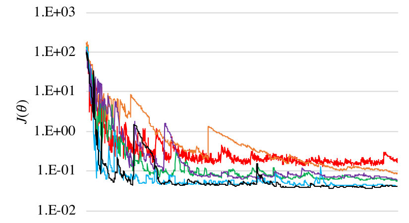 Figure 1
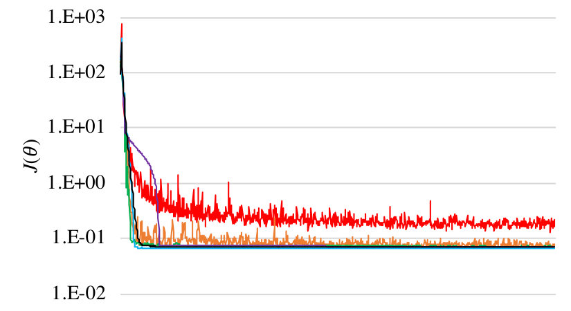 Figure 2
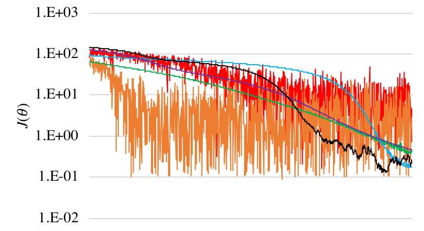 Figure 3
Peer Reviews
No public reviews on file for this paper yet. If you reviewed it on a platform where reviews are public (OpenReview, ICLR, NeurIPS, ICML), you can paste yours below so the community can read it here.
Videos
No videos yet. Explain this paper in a talk, walkthrough, or lecture? Add one.
Taxonomy
TopicsReinforcement Learning in Robotics · Advanced Bandit Algorithms Research · Adversarial Robustness in Machine Learning
**Sample Complexity of Estimating the Policy Gradient
for Nearly Deterministic Dynamical Systems**
Osbert Bastani
University of Pennsylvania, USA
Abstract
Reinforcement learning is a promising approach to learning robotics controllers. It has recently been shown that algorithms based on finite-difference estimates of the policy gradient are competitive with algorithms based on the policy gradient theorem. We propose a theoretical framework for understanding this phenomenon. Our key insight is that many dynamical systems (especially those of interest in robotics control tasks) are nearly deterministic—i.e., they can be modeled as a deterministic system with a small stochastic perturbation. We show that for such systems, finite-difference estimates of the policy gradient can have substantially lower variance than estimates based on the policy gradient theorem. Finally, we empirically evaluate our insights in an experiment on the inverted pendulum.
1 Introduction
The policy gradient is the workhorse of modern reinforcement learning. In particular, most state-of-the-art reinforcement learning algorithms aim to learn a control policy by estimating the policy gradient—i.e., the gradient of the expected cumulative reward with respect to the parameters of the control policy—in one of two ways: (i) numerically, e.g., using a finite-difference approximation (Kober et al., 2013; Mania et al., 2018), or (ii) by using the policy gradient theorem (Sutton et al., 2000) to construct estimates (Silver et al., 2014; Schulman et al., 2015a, b, 2017). However, there has been little work on theoretically understanding the tradeoffs between these two approaches, and our work aims to help fill this gap.
We are interested in applications to robotics control, which typically have continuous state and action spaces (Collins et al., 2005; Abbeel et al., 2007; Levine et al., 2016). For example, reinforcement learning can be used to learn controllers when the dynamics are unknown (Abbeel et al., 2007; Ross and Bagnell, 2012; Akametalu et al., 2014; Berkenkamp et al., 2017; Johannink et al., 2018). Understanding sample complexity is especially important in this application, since the goal is for robots to be able to learn based on real world experience, which can be very costly to obtain. Furthermore, having a theoretical understanding of sample complexity is important for developing safe reinforcement learning algorithms (Akametalu et al., 2014; Berkenkamp et al., 2017; Dean et al., 2018b).
We argue that near determinism is an important characteristic of dynamical systems relevant to robotics. More precisely, we study settings where the noise in the dynamics is “small” (i.e., sub-Gaussian with small constant). This setting captures robotics tasks such as grasping (Andrychowicz et al., 2018), quadcopters (Akametalu et al., 2014), walking (Collins et al., 2005), and driving (Montemerlo et al., 2008), where the dynamics are primarily deterministic but include small perturbations such as wind, friction, or slippage. We discuss this claim in detail below.
Main results. In the context of near determinism, we analyze the sample complexity of various algorithms for estimating the policy gradient . We study three algorithms: (i) an algorithm based on finite-differences, (ii) an algorithm based on the policy gradient theorem, and (iii) a model-based algorithm (i.e., it knows the system dynamics) that uses backpropagation to estimate the policy gradient. The model-based algorithm represents the best convergence rate we can hope to achieve using only random samples of the noise. We give details on these algorithms in Section 3.
Our key parameter of interest is the sub-Gaussian parameter of the system noise , which is small for nearly deterministic systems. Here, we also consider dependences on the estimation error and the dimension of the parameter space; we state theorems giving dependences on all parameters in Section 4. We prove the following bounds on the sample complexity (i.e., the number of samples needed to get at most error with probability at least ):
- •
For the model-based estimate, .
- •
For the finite-differences estimate, .
- •
For the estimate based on the policy gradient theorem, and .
Our key finding is that while both the model-based and finite-difference estimates become small as becomes small, the estimate based on the policy gradient theorem does not. Thus, for nearly deterministic dynamical systems, finite-difference algorithms perform significantly better. However, this improvement comes at a price— depends on , and furthermore quadratically more samples are needed to get to the same estimation error.
Finally, we focus on how many samples are needed to estimate the policy gradient on a single step. This understanding is already useful for applications such as safe reinforcement learning. Nevertheless, we discuss how our results connect to the problem of optimizing in Section 4.
Motivation for near determinism. A common approach in robotics is to model the robot dynamics as deterministic (Levinson et al., 2011; Kuindersma et al., 2016). To account for stochasticity, either a stabilizing controller such as a PID controller is used (Levinson et al., 2011), or the robot’s trajectory is replanned at every step (Kwon et al., 1983; Kuindersma et al., 2016). An alternative approach is to assume that the dynamics are deterministic plus a bounded perturbation at each step, and then use robust control (Akametalu et al., 2014). Both approaches implicitly assume that the deterministic portion of the dynamics are a good approximation of the full dynamics. In general, most systems that have been successfully studied in reinforcement learning are nearly deterministic, including Atari games (Mnih et al., 2015), MuJoCo benchmarks (Todorov et al., 2012; Levine and Koltun, 2013), and simulated grasping tasks (Andrychowicz et al., 2018).
More importantly, we believe that it will be challenging to increase the sample efficiency of reinforcement learning in systems where the noise is high. Indeed, our analysis shows that noise can be greatly amplified by the dynamics, so if the noise is large, we believe there is very little hope for sample-efficient reinforcement learning. In these settings, we may need to rely on techniques such as transfer learning (Taylor and Stone, 2009), meta-learning (Finn et al., 2017), or learning to plan (Tamar et al., 2016) to achieve low sample complexity.
Related work. The theoretical work in reinforcement learning algorithms has primarily focused on -learning (Watkins and Dayan, 1992; Kearns and Singh, 2002; Kakade et al., 2003; Jin et al., 2018), especially for Markov decision processes (MDPs) with finite state and action spaces. There has been some work on understanding the sample complexity of reinforcement learning with function approximation—e.g., for fitted value iteration (Munos and Szepesvári, 2008), for fitted policy iteration (Antos et al., 2008; Lazaric et al., 2012; Farahmand et al., 2015, 2016), fitted -iteration (Tosatto et al., 2017), and the algorithm (Dalal et al., 2018). For robotics tasks, where state and action spaces are typically continuous, the most successful approaches are predominantly based on policy gradient estimation (Collins et al., 2005; Kober et al., 2013), for which there has been relatively little work. In this direction, (Kakade et al., 2003) has analyzed the sample complexity of algorithms based on the policy gradient theorem, but they do not study the dependence of the sample complexity on the magnitude of the system noise. Furthermore, their work assumes finite state and action spaces and bounded rewards, and they do not consider finite-difference algorithms.
There has been work characterizing a key design choice of finite-difference algorithms—i.e., the distribution of perturbations used to numerically estimate the policy gradient (Roberts and Tedrake, 2009). They measure the performance of different choices using the signal-to-noise ratio. In contrast, our goal is to understand the sample complexity of different algorithms for nearly deterministic systems.
There has recently been work on understanding the sample complexity of learning controllers; however, they focus on linear dynamical systems, and on different algorithms—e.g., temporal difference learning (Tu and Recht, 2018b) or model-based algorithms (Dean et al., 2018a; Tu and Recht, 2018a). There has also been work in this setting studying the possibility of reducing variance by controlling the noise in the dynamics (Malik et al., 2019); in the setting we study, we cannot control the noise.
There has been recent work comparing approaches based on exploration in the action space (based on the policy gradient theorem) to exploration in the state space (based on finite difference methods) (Vemula et al., 2019). Our focus on nearly deterministic systems enables us to obtain qualitatively different insights compared to theirs. In particular, they find that approaches based on finite differences perform better for problems with a long time horizon. However, we analyze a more realistic model, and find that this insight no longer holds. Instead, approaches based on finite differences outperform approaches based on the policy gradient theorem for nearly deterministic systems.
Our analysis differs in three key ways. First, they assume an upper bound , which is a very strong assumption. Second, their analysis does not model stochastic dynamics. Instead, they assume that is deterministic, but they can only obtain observations , where is i.i.d. noise. In contrast, our analysis considers both stochastic dynamics, as well as how noise is propagated through the dynamics. This distinction substantially complicates our analysis, but is necessary for us to understand the implications of near determinism (since we need to understand how the dynamics can amplify noise). Finally, unlike their work, we provide lower bounds for our main results.
Connection to optimizing . Estimating the policy gradient can be used in conjunction with stochastic gradient descent to optimize . There is a large body of work on understanding the convergence rate of stochastic gradient descent (Robbins and Monro, 1985; Spall et al., 1992; Bottou and Bousquet, 2008; Moulines and Bach, 2011), of which policy gradient algorithms are a special case. Indeed, (Vemula et al., 2019) uses these techniques to bound the complexity of optimizing .
There are several reasons why we focus on understanding the sample complexity of a single gradient step rather than the sample complexity of optimization. First, they rely on the strong assumption that is bounded—i.e., for some . Second, it would be much more difficult to derive lower bounds on optimization—existing lower bounds are for the setting where the objective coming from a very general function family, and these bounds may not apply when is restricted to be the objective of a reinforcement learning problem. In contrast, for sample complexity, we derive matching (or almost matching) upper and lower bounds. Third, the sample complexity of estimating is of intrinsic interest—for example, it is an important prerequisite for safe reinforcement learning algorithms (Akametalu et al., 2014; Berkenkamp et al., 2017; Dean et al., 2018b). Finally, focusing on sample complexity simplifies our key insight. In particular, consider the the completely deterministic setting—optimizing a deterministic function using gradient descent may still take many steps, but “estimating” the gradient only requires a single sample.
Additionally, we note that sample complexity is directly related to the complexity of optimizing . In particular, the bounds in Vemula et al. (2019) all depend directly on the variance of the observations . Our proof bounds the sample complexity of estimating by bounding the sub-Gaussian parameter of , which is an upper bound on the variance of . Thus, smaller sample complexity translates to smaller complexity of optimizing .
Finally, our focus on estimating the gradient does not address the problem of exploration. In terms of optimization, gradient estimates can be used in conjunction with gradient descent to efficiently find local minima, whereas exploration is needed to find global minima. Understanding the sample complexity of exploration is an important but orthogonal problem that we leave to future work.
2 Preliminaries
We consider a dynamical system with states , actions , and transitions
[TABLE]
where is deterministic and is a random perturbation. We consider deterministic control policies with parameters . Except in the case of the model-based policy gradient algorithm, we assume that both and are unknown. We separate from since we are interested in settings where is small. Also, we that assume is independent of and . This assumption enables us to substantially simplify the model-based policy gradient (since we avoid taking a derivatives of ), and it also simplifies our analyses of other algorithms.
We are interested in controlling the system over a finite horizon —given a reward function , the goal is to find the policy that maximizes the expected cumulative reward
[TABLE]
where is the distribution over rollouts when using , and where we assume the initial state is deterministic and known. Note that is determined by and , so an expectation over is equivalent to one over . We are interested in estimating the policy gradient
[TABLE]
so we can perform gradient ascent on . As usual, let
[TABLE]
for , where , denote the function and value function, respectively (Sutton and Barto, 2018). In particular, .
Remark 2.1**.**
Our results straightforwardly extend to dynamical systems with time varying dynamics and rewards. Also, we can relax our assumption that the initial state is deterministic—i.e., to handle an initial state distribution , we can modify the dynamics on the first step to be , where and . Furthermore, our results can be extended to the case where the noise appears nonlinearly in the transitions, as long as it can be reparameterized (Kingma and Welling, 2014)—i.e., the transitions can be written in the form , where i.i.d. for some . We require that is Lipschitz in . Most kinds of noise considered in practice can be expressed in this form, though it may not satisfy the Lipschitz condition. Finally, our results can be extended to handle Martingale difference noise sequences by using the Azuma-Hoeffding inequality in place of the Hoeffding inequality.
3 Policy Gradient Algorithms
We now describe the policy gradient estimation algorithms that we consider.
Model-based policy gradient. When is known, we can estimate the policy gradient as
[TABLE]
since a rollout is determined by . In particular, we have estimator , where
[TABLE]
where i.i.d. for .
Policy gradient theorem. The policy gradient theorem is formulated for stochastic policies—i.e., is the probability of taking action in state . We assume a distribution of action perturbations that does not depend on —i.e., , where . Then, we have . The following are the modified and value functions:
[TABLE]
where as before. Then, the following is the policy gradient theorem (Sutton et al., 2000):
Theorem 3.1**.**
Letting be the distribution over rollouts when using , we have
[TABLE]
The key challenge to using Theorem 3.1 to estimate is to estimate . The simplest approach is to estimate it using a single rollout (Williams, 1992):
[TABLE]
A common technique to reduce variance is to normalize by subtracting the value function (Schulman et al., 2015b). In particular, the advantage function measures the advantage of using action instead of using in state at time . Then, we have
[TABLE]
Unlike , we cannot estimate using a single rollout. One approach is to estimate , and then estimate using . We assume that our estimate of is exact—in particular, we consider the following estimator :
[TABLE]
where i.i.d. for each .
Remark 3.2**.**
A common approach is to use an estimate of the function in place of . This approach reduces variance, but may introduce bias. For instance, for dynamical systems with continuous actions, the deterministic policy gradient (DPG) algorithm uses this approach Silver et al. (2014). We consider the algorithm described above for two reasons. First, our focus is on estimating the policy gradient, rather than understanding the sample complexity of -learning, which is required to analyze DPG. Second, it is hard to prove bounds for DPG since it relies on the derivative of the function, which cannot be bounded without additional assumptions. For example, suppose we train a random forest . Even if this model achieves achieves good accuracy, its gradient would be zero nearly everywhere since this model is piecewise constant; thus, it would not be useful in the context of the DPG algorithm.
Finite-difference policy gradient. We can use finite-differences to estimate .
Theorem 3.3**.**
For any (where ) where is -Lipschitz continuous, 111We assume the norm throughout.
[TABLE]
where (where is the Kronecker delta), and satisfies .
We give a proof in Appendix E. Then, the finite difference approximation of the policy gradient is
[TABLE]
We can estimate using samples , which yields the estimator , where
[TABLE]
where i.i.d. for and . Note that we use separate samples and to estimate and , respectively. If we are using a simulator, then we can reduce variance by using the same samples to estimate both terms.
Remark 3.4**.**
Typically, rather than choose a fixed set of basis vectors , finite-difference algorithms choose random vectors from a spherically symmetric distribution—e.g., (Spall et al., 1992; Mania et al., 2018). Our choice of a fixed basis simplifies our analysis.
4 Main Results
Sample complexity. Recall that the policy gradient must be estimated from sampled rollouts . Our goal is to understand the tradeoffs in sample complexity of estimating between various different reinforcement learning algorithms.
Definition 4.1**.**
Let be a random vector, and let , where i.i.d. The sample complexity of of is the smallest such that
[TABLE]
We are interested in the sample complexity of , where is an estimate of using a single rollout .
Assumptions. We let and . Similarly, for a stochastic policy (where ), we let and . Next, to ensure convergence, we make regularity assumptions about the dynamics and our control policy; see Appendix F & G for definitions.
Assumption 4.2**.**
We assume that , , , , , and are Lipschitz continuous and are twice continuously differentiable with Lipschitz continuous first derivative.
Remark 4.3**.**
This standard assumption is needed to ensure that we can estimate the gradient using finite differences. It is somewhat strong—e.g., it rules out commonly used quadratic rewards. In practice, the state space is often compact, in which case the Lipschitz continuity assumption becomes redundant. However, we cannot handle discontinuous rewards or dynamics (including piecewise constant rewards). In these cases, the policy gradient may diverge near the discontinuities; thus, the sample complexity of estimating this gradient may diverge as well. In principle, we could handle discontinuities as long as the policy visits these discontinuities with zero probability.
Finally, for any function , we let denote its Lipschitz constant and .
Assumption 4.4**.**
We assume that is -subgaussian.
This assumption is required for proving concentration—e.g., it is typically assumed in the context of safe reinforcement learning (Akametalu et al., 2014; Berkenkamp et al., 2017). In practice, perturbations due to noise are often bounded (which implies the noise is sub-Gaussian), especially for our setting of interest—e.g., forces due to wind, friction, or slippage have bounded magnituded. We are interested in settings where is small.
Definition 4.5**.**
A system is nearly deterministic if .
In particular, we are interested in the dependence of the sample complexity on .
Main theorems. For the model-based policy gradient, we have:
Theorem 4.6**.**
For , the sample complexity of satisfies
[TABLE]
For the policy gradient based on Theorem 3.1:
Theorem 4.7**.**
For the choice , has sample complexity
[TABLE]
where , for sufficiently small—i.e., . Next,
[TABLE]
The first lower bound holds for any that is everywhere differentiable on and satisfies , where is the sample complexity of estimating using samples from . The second lower bound holds for , for any .
We have shown two lower bounds—one for an arbitrary distribution (in terms of a sample complexity related to ), and one for the specific choice where is Gaussian (as is the case in our upper bound). Also, note that our upper bound depends on choosing the action noise to have variance . In principle, the first lower bound holds even if depends on the problem parameters; however, then may depend on these parameters as well. The second lower bound is independent of the the action noise , so it holds even if depends on the problem parameters.
Remark 4.8**.**
Note that the upper and lower bounds have a gap on the order of . We believe that this gap is due to limitations in our analysis. In particular, our lower bounds depend on a lower bound on the tail of the distribution, which has exponential tails. In contrast, our other lower bounds depend on Gaussian tails, which are doubly exponential. Intuitively, since the distribution has a longer tail, it should not have lower sample complexity.
Remark 4.9**.**
Note that the second lower bound contains a dependence on , which is unusual. However, this term only has a role if the first term in the minimum is very large. Furthermore, the first term depends as usual on (which is not shown since we omit log factors).
Remark 4.10**.**
Actor-critic approaches reduce variance by using function approximation to obtain lower variance estimates of the advantage (Schulman et al., 2015b). However, our lower bounds hold even if the advantage is known exactly. Thus, while actor-critic approaches can reduce variance, they do not affect our main insight that these estimates remain noisy for nearly deterministic dynamical systems.
For the finite-difference policy gradient:
Theorem 4.11**.**
The sample complexity of satisfies
[TABLE]
The first bound (i.e., the upper bound) holds for a choice . The second bound (i.e., the lower bound) holds for any , , and ,
Note that our upper bound is for the choice , but our lower bound holds for arbitrary .
Remark 4.12**.**
In an abuse of notation, in Theorem 4.11, we have ignored the fact that must always be at least ; in particular, it does not go to zero as goes to zero. This discrepancy in Theorem 4.11 arises because there is an implicit assumption we use when inverting Hoeffding’s inequality that —more precisely, Hoeffding’s inequality gives a bound of the form
[TABLE]
where is an estimate of using samples, and . Solving for yields . However, if , then is not well defined, so it does not mean we can get an estimate of using samples; instead, we need to take . In our proof of Theorem 4.11, we apply Hoeffding’s inequality times (since we estimate the gradient of each component separately), so we need .
Proof strategy. We give a high-level overview of our proof strategy, focusing on Theorem 4.6. Our proof proceeds in two steps. First, we prove an upper bound
[TABLE]
where and do not depend on . This step uses induction based on the recursive structure of . Second, we prove Lemma G.7; we state a simplified version:
Lemma 4.13**.**
Let be a -sub-Gaussian random vector over , and let be a random vector over satisfying , where . Then is -sub-Gaussian, where .
Combined with (1), we conclude that is sub-Gaussian, from which we can use Hoeffding’s inequality (see Lemma G.3) to complete the proof. For the lower bound, we construct a system where is Gaussian. The proof of Theorem 4.7 follows similarly, except we need to use analogous results for sub-exponential random variables. In particular, we prove Lemma H.7, an analog of Lemma G.7. The proof of Theorem 4.11 also follows similarly, but we need to account for the bias in the finite-difference estimate of from Theorem 3.3.
5 Discussion
Dependence on . Both and scale linearly in . Thus, the corresponding algorithms perform very well when is small. In contrast, does not become small when becomes small. Intuitively, if is wide, then the action noise adds uncertainty to . On the other hand, if is narrow, then becomes large—in particular, must change rapidly for some values of , and must have large gradient at such values of .
A key point is that in the first lower bound for (i.e., for arbitrary ), even though we do not know its explicit dependence on , , , and , we know that it is completely independent of . Thus, regardless of how is chosen (e.g., even if it chosen based on the problem parameters), the sample complexity does not become small as becomes small.
Full determinism (). When , we have (i.e., we only need a single sample to estimate ) and (i.e., we need two samples to estimate the derivative of each parameter, taking small enough to get error). For the case of , our lower bound in Theorem 4.7 still holds—the dynamical system we use to obtain the lower bound has no noise in the dynamics. In particular, a large number of samples are still needed to obtain good estimates (i.e., possibly exponential in ).
Dependence on . Both and depend quadratically on (ignoring the gap between the upper and lower bounds for ). In contrast, depends quartically on . This gap arises because according to Theorem 3.3, the finite-differences error of (assuming there is no noise) depends linearly on . Thus, we must choose to obtain error at most . If the dynamical system and control policy are both linear, then this error goes away, so the dependence on becomes quadratic.
Dependence on . Only depends on —whereas the other two algorithms make use of the fact that we can compute , the finite-difference approximation ignores this ability.
Dependence on . All of the sample complexities depend exponentially on . As we show in our lower bounds, this dependence is unavoidable—it arises from the fact that the dynamics cause the state (and therefore the rewards) to grow exponentially large in . A common assumption made in prior work is that the rewards are bounded uniformly by (Kearns and Singh, 2002; Kakade et al., 2003). Intuitively, our results indicate that without stronger assumptions, may be exponentially large. In practice, rewards for continuous control tasks are often quadratic, and can indeed be exponentially in magnitude.
An important aspect is that estimation is substantially easier when the current policy is good. In our bounds, the base of the exponential dependence is always . If the initial policy provides relatively stable control, then we may expect that —i.e., the states remain bounded in magnitude. Then, we have , so our bounds no longer depend exponentially on . This insight suggests the importance of good initialization for fast estimation.
Indeed, policy gradient estimators can have high variance in practice. As an example, consider the cart-pole problem with continuous action space, with random initial state and where the reward function is the negative distance to origin. We empirically estimated that the MSE of the model-based policy gradient estimator using on a randomly initialized policy for this benchmark is . This error is substantially reduced when the policy is stable—for a trained cart-pole policy, we estimate that the MSE of the model-based policy gradient estimator is just .
6 Experiments
We empirically evaluated the effect of on the performance of the different algorithms.
Dynamical system. We use the inverted pendulum (Tedrake, 2018) (specifically, using the dynamics from OpenAI Gym (Brockman et al., 2016)), which has state space (i.e., angle and angular velocity ) and actions (i.e., applied torque). Letting be the (deterministic) pendulum dynamics, we consider the system , where i.i.d. We use the rewards
[TABLE]
where is the angle corresponding to the upright position, and , , and . Our goal is to control the system over a horizon of steps, from a fixed start state , where . For the control policy, we used a neural network with a single hidden layer with 100 neurons, ReLU activations, and linear outputs. As usual, we randomly initialize the weights; to reduce variance, we initialized the policy to have a reasonably high reward by running our model-based algorithm until .
Algorithms. We use stochastic gradient descent in conjunction with each of the three estimation algorithms. On each gradient step, we use a single sample to estimate the gradient, and we take 1000 gradient steps. We modify the finite-difference algorithm to use a single random sample (i.e., the uniform distribution on the unit sphere in ), rather than summing over the basis vectors . This choice may improve the dependence of the sample complexity on ; however, it should not affect dependence on , which is our parameter of interest.
For the algorithm based on the policy gradient theorem, we use action noise . For each choice of , we used cross-validation to identify the optimal hyperparameters: the learning rate (for all algorithms), the parameter (for the finite-differences algorithm), and the action noise (for the algorithm based on the policy gradient theorem).
Results. Average the results of each algorithm over 20 runs; the algorithms have very high variance, so we discard runs that do not converge. In Figure 1, we show the learning curves for (i.e., as a function of the number of gradient steps). The darker colors correspond to smaller noise. We show enlarged versions of these plots in Appendix I.
Note that unlike the other two algorithms, the finite-difference algorithm actually uses 2000 sampled rollouts (since it uses two per gradient step). However, this detail does not affect our insights regarding the relative convergence rate of different algorithms for different .
Our key finding is that the learning curves for the model-based and finite-differences are ordered based on the choice of —i.e., the curves tend to converge more quickly for smaller choices of . This effect is most apparent in the curves for the finite-differences algorithms, where curves for smaller (black and blue) converge much faster than those for larger (red and orange). In contrast, the learning curves for the policy gradient based algorithm do not have strong dependence on . For example, the fastest curve to converge (at least initially) for the policy gradient based algorithm is for our second-largest choice (orange), whereas the slowest to converge is for (blue). These results mirror our theoretical insights.
Finally, as expected, the model-based algorithm converges most quickly, followed by the finite-differences and policy gradient theorem based algorithms.
7 Conclusion
We have analyzed the sample complexity of algorithms for estimating the policy gradient for nearly deterministic dynamical systems. Future work includes leveraging these results in safe reinforcement learning algorithms, and understanding the sample complexity of optimizing .
Acknowledgements
This work was supported by NSF CCF-1910769.
Appendix A Proof of Theorem 4.6
Preliminaries.
Note that the expected cumulative reward is equivalent to
[TABLE]
and the expected model-based policy gradient is
[TABLE]
Similarly, given a sample , the stochastic approximation of the expected cumulative reward is
[TABLE]
and the stochastic approximation of the model-based policy gradient is
[TABLE]
Bounding the deviation of from .
We claim that for , we have
[TABLE]
for all and , where
[TABLE]
where is a Lipschitz constant for . The base case follows trivially. Note that . Then, for , we have
[TABLE]
Similarly, we have
[TABLE]
The claim follows.
Bounding the deviation of from .
We claim that
[TABLE]
where . To this end, letting , note that
[TABLE]
for , so
[TABLE]
where the last step follows from our bound on in Lemma D.2.
Upper bound on sample complexity of .
Note that , where we think of as the length concatenation of the vectors , so is -sub-Gaussian. We apply Lemma G.7 with
[TABLE]
Thus, is -sub-Gaussian, where
[TABLE]
Thus, by Lemma G.6, the sample complexity of is
[TABLE]
The claim follows.
Lower bound on sample complexity of .
Consider a linear dynamical system with , time-invariant deterministic transitions (where ), time-varying noise
[TABLE]
where , initial state , time-varying rewards
[TABLE]
control policy class , and current parameters . Note that
[TABLE]
where is the noise on the first step. Thus, we have
[TABLE]
so
[TABLE]
Also, note that
[TABLE]
Next, note that for i.i.d. samples , we have
[TABLE]
where
[TABLE]
Thus, by Lemma G.8, for
[TABLE]
we have
[TABLE]
Thus, the sample complexity of satisfies
[TABLE]
Note that the numerator is positive as long as . The claim follows, as does the theorem statement. ∎
Appendix B Proof of Theorem 4.7
Preliminaries.
Recall the form of the policy gradient based on Theorem 3.1:
[TABLE]
where, for , we have
[TABLE]
where
[TABLE]
The stochastic approximation of for a single sampled rollout is
[TABLE]
Bounding .
We claim that
[TABLE]
where
[TABLE]
where is a Lipschitz constant for . We prove by induction. The base case is trivial. Note that , and similarly . Then, for , we have
[TABLE]
The claim follows.
Bounding .
We claim that
[TABLE]
where . Recall that . Thus, we have
[TABLE]
Thus, we have
[TABLE]
as claimed.
Bounding the deviation of from .
We claim that
[TABLE]
where , , and . First, note that
[TABLE]
where the last step follows from the bound on in Lemma D.3. Then, we have
[TABLE]
Furthermore, we have
[TABLE]
where we have used the fact that , and similarly . Therefore, we have
[TABLE]
as claimed.
Upper bound on the sample complexity of .
We have , where we think of as the values , , and , for all , , and . Since and are -sub-Gaussian for each , by Lemma H.6, is -sub-exponential, where . Thus, we can apply Lemma H.7 with
[TABLE]
Thus, is -sub-exponential, where
[TABLE]
Thus, by Lemma G.6, the sample complexity of is
[TABLE]
for all . The claim follows.
Lower bound on the sample complexity of .
Consider a linear dynamical system with , time-varying deterministic transitions
[TABLE]
zero noise (i.e., ), initial state , time-varying rewards
[TABLE]
control policy class , current parameters , and action noise . Note that
[TABLE]
where i.i.d., so
[TABLE]
where is the action noise on the first step. Note that
[TABLE]
and
[TABLE]
In particular, note that
[TABLE]
Also, note that . Therefore, we have
[TABLE]
Thus, for i.i.d. samples , we have
[TABLE]
Note that for satisfying our conditions (differentiable on and satisfying ), we have
[TABLE]
where the second-to-last step follows from integration by parts. Thus, by the definition of the sample complexity,
[TABLE]
for any , so we have
[TABLE]
for any . Thus, we have
[TABLE]
Next, consider the case where , for any . Then, we have
[TABLE]
so
[TABLE]
where are i.i.d. standard Gaussian random variables for . By Lemma H.8, letting (so ), for
[TABLE]
we have
[TABLE]
Thus, the sample complexity of satisfies
[TABLE]
Note that the numerator is positive as long as . The claim follows, as does the theorem statement. ∎
Appendix C Proof of Theorem 4.11
Preliminaries.
Note that the expected cumulative reward is equivalent to
[TABLE]
Similarly, given a sample , the stochastic approximation of the expected cumulative reward is
[TABLE]
The finite difference approximation of is
[TABLE]
where is a basis vector for and is the dimension of the parameter space . Finally, an estimate of the finite difference approximation for two samples is
[TABLE]
where is as defined in the proof of Theorem 4.6.
Bounding the deviation of from .
We claim that for , we have
[TABLE]
for all and , where
[TABLE]
where is a Lipschitz constant for . The base case follows trivially. Note that . Then, for , we have
[TABLE]
The claim follows.
Bounding the deviation of from .
Let
[TABLE]
Then, letting , note that
[TABLE]
where . Thus, we have
[TABLE]
for , where .
Upper bound on the sample complexity of .
Note that , where is the length concatenation of the vectors , so is -sub-Gaussian. We apply Lemma G.7 with
[TABLE]
Thus, is -sub-Gaussian, where
[TABLE]
Thus, by Lemma G.6, for , the sample complexity of is
[TABLE]
Upper bound on the sample complexity of .
By Theorem 3.3, we have
[TABLE]
where
[TABLE]
where the second inequality follows from the fact that and the bound on in Lemma D.2. Now, taking
[TABLE]
then with probability , we have
[TABLE]
so the sample complexity of is
[TABLE]
The claim follows.
Lower bound on the sample complexity of .
Consider a linear dynamical system with , , time-varying deterministic transitions
[TABLE]
time-varying noise
[TABLE]
where , initial state , time-varying rewards
[TABLE]
where is defined by
[TABLE]
control policy class , and current parameters . Note that technically, is not twice continuously differentiable, so it does not satisfy Assumption 4.2. However, the only place in the proof of Theorem 4.11 where we need this assumption is to apply Lemma F.2 in Lemma D.2. By the discussion in the proof of Lemma F.2, the lemma still applies, so our theorems still apply to this dynamical system. Now, we have
[TABLE]
where is the noise on the first step. Thus, we have
[TABLE]
Also, note that
[TABLE]
so , since .
Next, note that for i.i.d. samples , we have
[TABLE]
Letting for , and using the fact that , we have
[TABLE]
where
[TABLE]
Thus, by Lemma G.8, for
[TABLE]
and recalling that , we have
[TABLE]
Thus, the sample complexity of satisfies
[TABLE]
Now, recall that , so
[TABLE]
Thus, using our assumption , then we need to have for to hold. As a consequence, using our assumption , we must have
[TABLE]
where the last step follows since implies . Thus, we have , so we have . Finally, we have
[TABLE]
so the sample complexity of satisfies
[TABLE]
Finally, for any , we can consider independent copies of this dynamical system. Then, estimating the gradient is equivalent to estimating for each . Thus, we have
[TABLE]
The claim follows, as does the theorem statement. ∎
Appendix D Bounds on Lipschitz Constants
We prove bounds on the Lipschitz constants for , for , and for . We use implicitly use the commonly known results in Appendix F throughout these proofs.
Lemma D.1**.**
We claim that for , is -Lipschitz, where
[TABLE]
Proof.
First, we show that is -Lipschitz in and -Lipschitz in , where
[TABLE]
We prove by induction. The base case is trivial. Then, for , note that is -Lipschitz in , where
[TABLE]
Similarly, note that is -Lipschitz in , where
[TABLE]
as was to be shown. Finally, note that
[TABLE]
so
[TABLE]
Thus, is -Lipschitz, where
[TABLE]
The claim follows. ∎
Lemma D.2**.**
We claim that for , is -Lipschitz, where
[TABLE]
Proof.
First, we show that is -Lipschitz in and -Lipschitz in , and that is -Lipschitz in and -Lipschitz in , where
[TABLE]
We prove by induction. The base case is trivial. First, for , note that is -Lipschitz in , where
[TABLE]
Second, note that is -Lipschitz in , where
[TABLE]
Third, note that is -Lipschitz in , where
[TABLE]
Fourth, note that is -Lipschitz in , where
[TABLE]
as was to be shown. Finally, note that
[TABLE]
so
[TABLE]
so
[TABLE]
Thus, is -Lipschitz, where
[TABLE]
The claim follows. ∎
Lemma D.3**.**
We claim that for , is -Lipschitz, where
[TABLE]
Proof.
Note that is exactly equal to with replaced with and replaced with . Thus, the claim follows by the same argument as for Lemma D.1. ∎
Appendix E Proof of Theorem 3.3
Theorem E.1**.**
(Taylor’s theorem) Let be an everywhere differentiable function with -Lipschitz derivative. Then, for any , we have
[TABLE]
where
[TABLE]
Proof.
The claim follows from Theorem 5.15 in Rudin et al. (1976), together with Lemma F.2, which implies that for all . ∎
Now, we prove Theorem 3.3. By Taylor’s theorem, we have
[TABLE]
where
[TABLE]
Thus, we have
[TABLE]
Therefore, we have
[TABLE]
so
[TABLE]
as claimed. ∎
Appendix F Technical Lemmas (Lipschitz Constants)
We define Lipschitz continuity (for the norm), and prove a number of standard results.
Definition F.1**.**
A function (where and ) is -Lipschitz continuous if for all ,
[TABLE]
If is a space of matrices or tensors, we assume and are unrolled into vectors. in (3).
Lemma F.2**.**
If is -Lipschitz and continuously differentiable, then for all ,
[TABLE]
Proof.
Note that
[TABLE]
so
[TABLE]
as claimed. Note that the result holds even if each component is continuously differentiable except on a finite set . In particular, for each point , we can use the standard definition , where is the right derivative and is the left deriviative. Letting and , then . Then, we have
[TABLE]
as claimed. ∎
Lemma F.3**.**
If are - and -Lipschitz, respectively, then is -Lipschitz, where .
Proof.
Note that
[TABLE]
as claimed. ∎
Lemma F.4**.**
If where is -Lipschitz and bounded by (i.e., for all ), and is -Lipschitz and bounded by . Then is -Lipschitz, where .
Proof.
Note that
[TABLE]
as claimed. ∎
Lemma F.5**.**
If is -Lipschitz and is -Lipschitz, then is -Lipschitz, where .
Proof.
Note that
[TABLE]
as claimed. ∎
Lemma F.6**.**
Let be -Lipschitz in (for all ) and -Lipschitz in (for all ). Then, is -Lipschitz in , where .
Proof.
Note that
[TABLE]
as claimed. ∎
Lemma F.7**.**
Let be -Lipschitz, and be -Lipchitz. Then, is -Lipschitz, where .
Proof.
Note that
[TABLE]
as claimed. ∎
Lemma F.8**.**
Let be -Lipschitz. Then, (where is a distribution over ) is -Lipschitz, where .
Proof.
Note that
[TABLE]
as claimed. ∎
Appendix G Technical Lemmas (Sub-Gaussian Random Variables)
We define sub-Gaussian random variables, and prove a number of standard results. We also prove Lemma G.7, a key lemma that enables us to infer a sub-Gaussian constant for a random variable bounded in norm by a sub-Gaussian random variable , i.e., (where is the norm). This lemma is a key step in the proofs of our upper bounds for the model-based and finite-difference policy gradient estimators. Finally, we also prove Lemma G.8, which is a key step in the proof of our lower bounds.
Definition G.1**.**
A random variable over is -sub-Gaussian if , and for all , we have .
Lemma G.2**.**
If a random variable over is -sub-Gaussian, then .
Proof.
See Stromberg (1994). ∎
Lemma G.3**.**
(Hoeffding’s inequality) Let be i.i.d. -sub-Gaussian random variables over . Then,
[TABLE]
Proof.
See Proposition 2.1 of Wainwright (2019). ∎
Definition G.4**.**
A random vector over is -sub-Gaussian if each is -sub-Gaussian.
Lemma G.5**.**
If a random vector over is -sub-Gaussian, then .
Proof.
Note that
[TABLE]
where the first inequality follows from Jensen’s inequality. ∎
Lemma G.6**.**
Let be random vector over with mean , such that is -sub-Gaussian. Then, given , the sample complexity of satisfies
[TABLE]
i.e., given i.i.d. samples of with empirical mean , then .
Proof.
Note that
[TABLE]
as claimed. ∎
Lemma G.7**.**
Let be a -sub-Gaussian random vector over , and let be a random vector over satisfying
[TABLE]
where . Then is -sub-Gaussian, where
[TABLE]
Proof.
We first prove that is bounded for each , and then use this fact to prove that is sub-Gaussian. In particular, we claim that for any and any , we have
[TABLE]
where
[TABLE]
To this end, note that by Theorem 5.1 in Lattimore and Szepesvári (2018), for any and any , we have
[TABLE]
Now, note that
[TABLE]
We consider three cases. First, suppose that . Then, , so
[TABLE]
Furthermore, , so
[TABLE]
Second, if , then
[TABLE]
so
[TABLE]
Third, if , then
[TABLE]
so
[TABLE]
As a consequence, by Note 5.4.2 in Lattimore and Szepesvári (2018), is -sub-Gaussian. Note that , so the theorem follows. ∎
Lemma G.8**.**
Given ,
[TABLE]
Proof.
By Theorem 2 in Chang et al. (2011), we have
[TABLE]
where is the cumulative distribution function of . Thus, for , we have
[TABLE]
The claim follows. ∎
Appendix H Technical Lemmas (Sub-Exponential Random Variables)
We define sub-exponential random variables, and prove a number of standard results. Additionally, we prove Lemma H.7 (an analog of Lemma G.7), a key lemma that enables us to infer a sub-exponential constant for a random variable bounded in norm by a sub-exponential random variable , i.e., (where is the norm). This lemma is a key step in the proof of our upper bound in Theorem 4.7. Finally, we also prove Lemma H.8, which is a key step in the proof of our lower bound in Theorem 4.7.
Definition H.1**.**
A random variable over is -sub-exponential if , and for all satisfying , we have .
Lemma H.2**.**
Let be i.i.d. -sub-exponential random variables over . Then, we have
[TABLE]
Proof.
See (2.20) in Wainwright (2019). ∎
Definition H.3**.**
A random vector over is -sub-exponential if each is -sub-exponential.
Lemma H.4**.**
Let be a random vector over with mean , such that is -sub-exponential. Then, given such that , the sample complexity of satisfies
[TABLE]
i.e., given i.i.d. samples of with empirical mean , then .
Proof.
Note that
[TABLE]
as claimed. ∎
Lemma H.5**.**
Let be -sub-Gaussian. Then, is -sub-exponential, where .
Proof.
The result follows from Lemma 5.5, Lemma 5.14, and the discussion preceding Definition 5.13 in Vershynin (2010). In particular, using the notation in Vershynin (2010), by Lemma 5.5, we have that satisfies . Then, by Lemma 5.14, we have that . Finally, by the discussion preceding Definition 5.13, we have that is -sub-exponential with parameters . The claim follows. ∎
Lemma H.6**.**
Let and be -sub-Gaussian, respectively. Then, is -sub-exponential, where .
Proof.
Note that
[TABLE]
By Lemma H.5, we have and are -sub-exponential for , so is -sub-exponential, for , as claimed. ∎
Lemma H.7**.**
Let be a -sub-exponential random vector over , and let be a random vector over satisfying
[TABLE]
where . Then is -sub-exponential, where .
Proof.
We use Lemma 5.14 and the discussion preceding Definition 5.13 in Vershynin (2010). In particular, let ; then, from the definition of sub-exponential random variables with , we have
[TABLE]
for each . Thus, using the notation in Vershynin (2010), so by the discussion preceding the Definition 5.13 in Vershynin (2010), we have satisfies , and furthermore satisfies
[TABLE]
for all , where . Thus, for each , we have
[TABLE]
Now, let
[TABLE]
We consider three cases. First, suppose that . Then, , so
[TABLE]
Furthermore, , so
[TABLE]
Second, if , then
[TABLE]
so
[TABLE]
Third, if , then
[TABLE]
so
[TABLE]
As a consequence, by the discussion preceding Definition 5.13 in Vershynin (2010), we have satisfies . Thus, by Lemma 5.15 in Vershynin (2010), we have that is -sub-exponential, where
[TABLE]
The claim follows. ∎
Lemma H.8**.**
Given , let
[TABLE]
where i.i.d., and let . Then, we have
[TABLE]
Proof.
Let be the sum of the squares of i.i.d. standard Gaussian random variables . We assume that is even. Then, is distributed according to the distribution, which has density function
[TABLE]
and mean . For , we have
[TABLE]
where the second inequality follows from a result
[TABLE]
based on Stirling’s approximation Robbins (1955). Thus, for any , we have
[TABLE]
Finally, for , where i.i.d., note that and
[TABLE]
so we have
[TABLE]
The claim follows. ∎
Appendix I Experimental Results
We show enlarged versions of the plots from Figure 1:
Model-Based Algorithm
Finite-Differences Algorithm
Policy Gradient Theorem Algorithm
The reference list from the paper itself. Each links out to its DOI / PubMed record.
- 1Abbeel et al. (2007) Pieter Abbeel, Adam Coates, Morgan Quigley, and Andrew Y Ng. An application of reinforcement learning to aerobatic helicopter flight. In Advances in neural information processing systems , pages 1–8, 2007.
- 2Akametalu et al. (2014) Anayo K Akametalu, Shahab Kaynama, Jaime F Fisac, Melanie Nicole Zeilinger, Jeremy H Gillula, and Claire J Tomlin. Reachability-based safe learning with gaussian processes. In CDC , pages 1424–1431. Citeseer, 2014.
- 3Andrychowicz et al. (2018) Marcin Andrychowicz, Bowen Baker, Maciek Chociej, Rafal Jozefowicz, Bob Mc Grew, Jakub Pachocki, Arthur Petron, Matthias Plappert, Glenn Powell, Alex Ray, et al. Learning dexterous in-hand manipulation. ar Xiv preprint ar Xiv:1808.00177 , 2018.
- 4Antos et al. (2008) András Antos, Csaba Szepesvári, and Rémi Munos. Learning near-optimal policies with bellman-residual minimization based fitted policy iteration and a single sample path. Machine Learning , 71(1):89–129, 2008.
- 5Berkenkamp et al. (2017) Felix Berkenkamp, Matteo Turchetta, Angela Schoellig, and Andreas Krause. Safe model-based reinforcement learning with stability guarantees. In Advances in Neural Information Processing Systems , pages 908–918, 2017.
- 6Bottou and Bousquet (2008) Léon Bottou and Olivier Bousquet. The tradeoffs of large scale learning. In Advances in neural information processing systems , pages 161–168, 2008.
- 7Brockman et al. (2016) Greg Brockman, Vicki Cheung, Ludwig Pettersson, Jonas Schneider, John Schulman, Jie Tang, and Wojciech Zaremba. Openai gym. ar Xiv preprint ar Xiv:1606.01540 , 2016.
- 8Chang et al. (2011) Seok-Ho Chang, Pamela C Cosman, and Laurence B Milstein. Chernoff-type bounds for the gaussian error function. IEEE Transactions on Communications , 59(11):2939–2944, 2011.