A priori error estimates for the finite element approximation of Westervelt's quasilinear acoustic wave equation
Vanja Nikoli\'c, Barbara Wohlmuth

TL;DR
This paper provides a priori error estimates for finite element approximations of Westervelt's quasilinear acoustic wave equation, demonstrating optimal convergence rates through theoretical analysis and numerical experiments.
Contribution
It introduces a novel a priori error analysis for finite element discretization of Westervelt's equation using Banach fixed-point theorem and inverse estimates.
Findings
Optimal convergence rates in $L^2$ norms for small data and mesh size.
Numerical experiments confirm theoretical error estimates.
Method avoids degeneracy issues in semi-discrete equations.
Abstract
We study the spatial discretization of Westervelt's quasilinear strongly damped wave equation by piecewise linear finite elements. Our approach employs the Banach fixed-point theorem combined with a priori analysis of a linear wave model with variable coefficients. Degeneracy of the semi-discrete Westervelt equation is avoided by relying on the inverse estimates for finite element functions and the stability and approximation properties of the interpolation operator. In this way, we obtain optimal convergence rates in -based spatial norms for sufficiently small data and mesh size and an appropriate choice of initial approximations. Numerical experiments in a setting of a 1D channel as well as for a focused-ultrasound problem illustrate our theoretical findings.
Click any figure to enlarge with its caption.
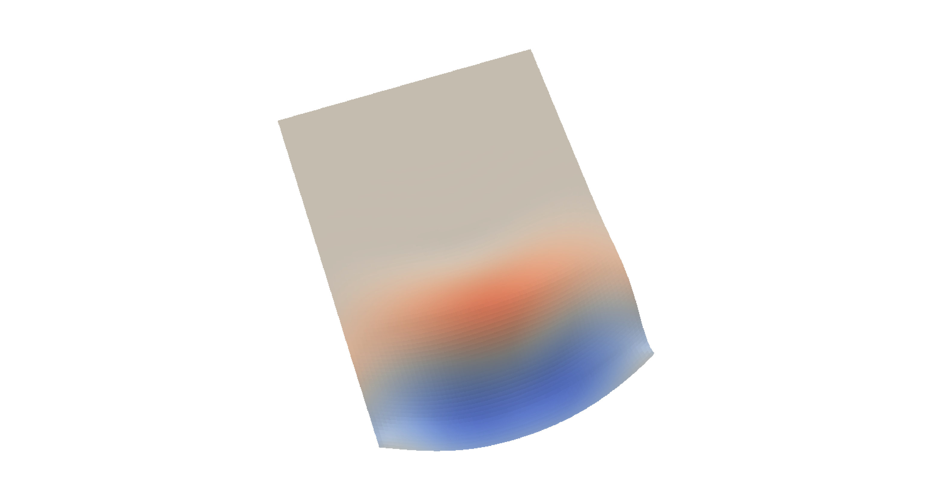 Figure 1
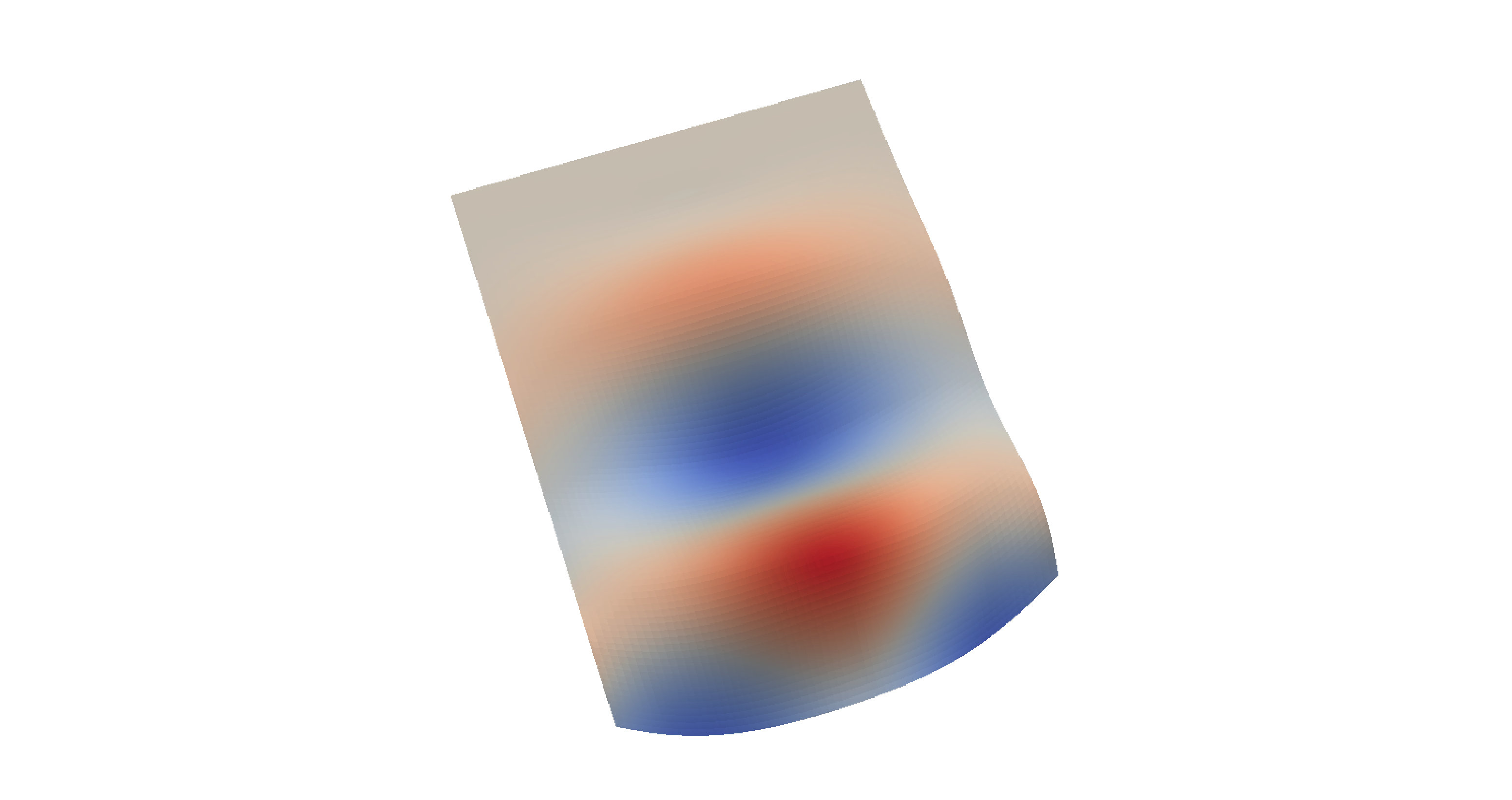 Figure 2
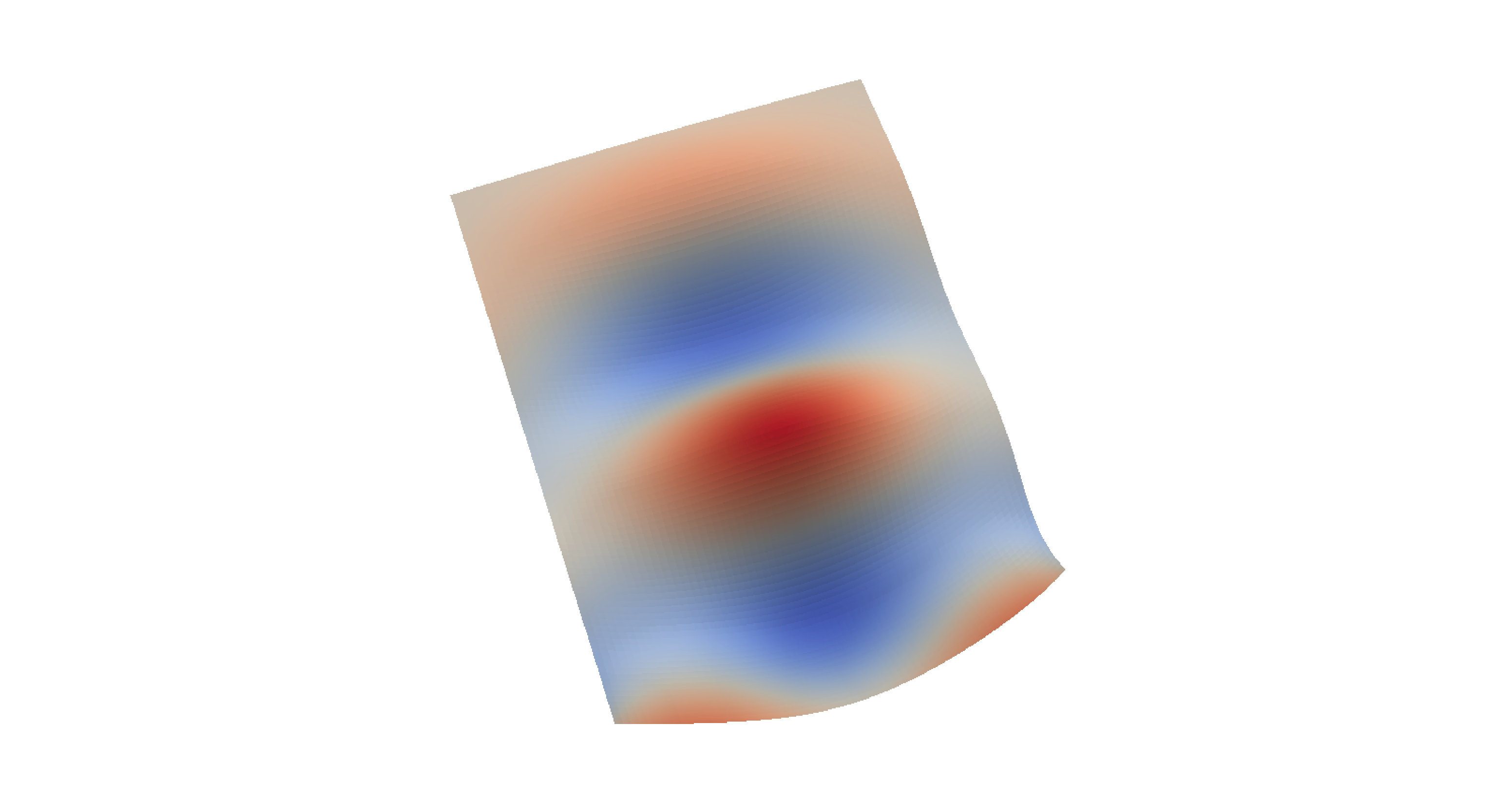 Figure 3
Peer Reviews
No public reviews on file for this paper yet. If you reviewed it on a platform where reviews are public (OpenReview, ICLR, NeurIPS, ICML), you can paste yours below so the community can read it here.
Videos
No videos yet. Explain this paper in a talk, walkthrough, or lecture? Add one.
\newsiamremark
remarkRemark \newsiamremarkhypothesisHypothesis
\newsiamthmclaimClaim \newsiamremarkassumptionAssumption \headersA priori error estimates for Westervelt’s wave equationV. Nikolić and B. Wohlmuth
A priori error estimates for the finite element approximation of Westervelt’s quasilinear acoustic wave equation
Vanja Nikolić22footnotemark: 2
Barbara Wohlmuth22footnotemark: 2
Abstract
We study the spatial discretization of Westervelt’s quasilinear strongly damped wave equation by piecewise linear finite elements. Our approach employs the Banach fixed-point theorem combined with a priori analysis of a linear wave model with variable coefficients. Degeneracy of the semi-discrete Westervelt equation is avoided by relying on the inverse estimates for finite element functions and the stability and approximation properties of the interpolation operator. In this way, we obtain optimal convergence rates in -based spatial norms for sufficiently small data and mesh size and an appropriate choice of initial approximations. Numerical experiments in a setting of a 1D channel as well as for a focused-ultrasound problem illustrate our theoretical findings.
keywords:
finite element method, a priori analysis, nonlinear acoustics, Westervelt’s equation
{AMS}
35L05, 65M15, 65M60
†††Technical University of Munich, Department of Mathematics, Chair of Numerical Mathematics, Boltzmannstraße 3, 85748 Garching, Germany (, ).
1 Introduction
The goal of the present work is to analyze a spatial discretization by piecewise linear finite elements in nonlinear acoustics. To this end, we study a discretization of Westervelt’s wave equation for the acoustic pressure
[TABLE]
which represents a classical model for nonlinear ultrasound propagation through thermoviscous fluids [53]. Our research is motivated by a rising number of nonlinear ultrasound applications in medicine and industry [4, 15, 37, 39, 41]. In (1), the constant denotes the speed of sound, is the sound diffusivity, and , where is the mass density and the coefficient of nonlinearity of the medium.
Westervelt’s equation is a strongly damped quasilinear wave equation with potential degeneracy due to the factor next to the second time derivative. For its derivation and the theoretical foundations of nonlinear acoustics, we refer to [9, 13, 20, 53], while results on the existence of smooth solutions of (1) can be found in [25, 26, 34]. Efficient simulation of the Westervelt equation and, in general, nonlinear sound propagation by the finite element method has been an active area of research. We refer to, e.g., [16, 22, 24, 29, 35, 36, 50, 52], which all focus on algorithmic aspects of finite element discretizations without any a priori analysis.
Error analysis for the standard finite element discretization of linear wave equations is an extensively studied topic; see, e.g., [1, 2, 3, 11, 18, 32, 49] and the references given therein. In particular, we single out the work on a priori analysis in [1] which provides error estimates for the undamped linear wave equation and the results on error bounds for strongly damped linear wave equations [32, 49]. Results on a class of nonlinear wave equations of a divergent type are also well-established. In [10], error analysis is provided for a semi-discretization of nonlinear wave equations of the form
[TABLE]
with a monotonicity condition on the corresponding bilinear form; cf. [10, Theorem 3.2]. In [47], semi-discretization for the following damped model is considered
[TABLE]
with . In [12], convergence of a full discretization for a class of nonlinear second-order in time evolution equations is provided where the operator acting on the first time derivative is assumed to be hemicontinuous, monotone, coercive, and to fulfill a certain growth condition. Moreover, the operator acting on the solution is assumed to be linear, bounded, symmetric, and strongly positive. We also mention the results in [33] on a class of problems of nonlinear elastodynamic and in [40] on the discontinuous Galerkin methods for a class of divergent-type nonlinear hyperbolic equations.
This work contributes to the finite element analysis of Westervelt’s equation in two ways. We first prove that, coupled with non-zero initial conditions and homogeneous Dirichlet data, its semi-discretization by piecewise linear finite elements has a unique solution which remains bounded in an appropriately chosen norm. Secondly, we derive an optimal a priori error estimate that has the form
[TABLE]
where . Our results are intended to enhance the numerical analysis of strongly damped quasilinear wave equations where the nonlinearities in the equation involve the time derivatives of the solution. We note that a particular feature of the present quasilinear equation is that the non-degeneracy is not a priori given. In our proofs we have to ensure that the factor next to the second time derivative remains positive.
In the continuous analysis of the Westervelt equation, non-degeneracy is typically achieved by a higher-regularity result for the solution and the use of an embedding, e.g., ; see [25, Theorem 3.1]. Such a strategy is not possible here since we use piecewise linear basis functions. Instead we employ inverse estimates for finite element functions and the stability and approximation properties of the Scott–Zhang interpolation operator [44].
Our analysis relies on the Banach fixed-point theorem combined with error estimates for a linear wave equation with variable coefficients. Therefore, in this work, we also obtain error estimates for strongly damped variable coefficient wave equations that take coefficient error into account as relevant, e.g., in optimal control problems in nonlinear acoustics [7, 28, 36].
The rest of the paper is organized as follows. Section 2 introduces the notation and lays out the most important theoretical results in Sobolev and finite element spaces that we often use in the analysis. In Section 3, we discuss the continuous problem and its well-posedness. In Section 4, we then study a linearized Westervelt equation with variable coefficients and prove that its semi-discretization has a unique solution. Section 5 focuses on the a priori analysis of this linear model. In Section 6, we show well-posedness and derive convergence rates for the semi-discrete Westervelt equation. Finally, Section 7 contains numerical examples that illustrate our theory.
2 Theoretical preliminaries
We begin by setting the notation and summarizing some auxiliary properties of Sobolev and finite element spaces that we will frequently use in the analysis.
2.1 Notation
We denote the standard inner product by . The norms in Sobolev spaces and are denoted by and , respectively, where , . The norms in Bochner spaces are denoted by , where , . We also introduce the spaces , for .
The constants , , appearing in the estimates denote generic constants that might depend on the coefficients in the equation and the domain , but not on the mesh size. Throughout the paper, we assume to be a fixed time horizon.
2.2 Auxiliary inequalities
Let , where , be a bounded domain with Lipschitz regular boundary. The nonlinear terms appearing in the Westervelt equation are of a quadratic type, so after variational testing, we often have to employ Hölder’s inequality for a product of three functions. In particular, we frequently make use of the following three special cases of Hölder’s inequality:
[TABLE]
with . We also often employ a special case of Young’s -inequality in the form
[TABLE]
see [14, Appendix B]. Let and be non-negative continuous functions and non-negative constants such that
[TABLE]
Then the following modification of Gronwall’s inequality holds
[TABLE]
see [17, Lemma 3.1]. Finally, we recall the Sobolev embeddings
[TABLE]
for , where , noting that .
2.3 Finite element spaces
We consider the discretization in space by continuous piecewise linear finite elements that vanish on the boundary. Let , , be a convex polygonal domain. For , let be a triangulation of made of triangles (in ) or of tetrahedrons (in ) so that . We denote by the space of polynomials on of degree no greater than . We introduce the finite element space as
[TABLE]
We assume that is a quasiuniform family: there are constants such that
[TABLE]
where denotes the diameter of the triangle (tetrahedron) K, stands for the diameter of the greatest ball (sphere) included in K, and
It is known that there exists and such that
[TABLE]
for , ; see [19].
Inverse estimates. Under the assumptions made above on the family , there is a such that
[TABLE]
for every ; see [5, Theorem 4.5.11]. We will need the special cases and in the proofs.
Bounds for the interpolation error. In our analysis, we will employ an interpolant of Scott–Zhang type, where , ; cf. [5, 44]. The following approximation and stability properties hold:
[TABLE]
where ; see [5, Theorem 4.8.12 and Corollary 4.8.15].
3 The continuous problem
We start from the following initial-boundary value problem for the Westervelt equation
[TABLE]
The weak form of the problem is then given by
[TABLE]
This problem is known to be well-posed for small data.
Theorem 3.1**.**
[25, Theorem 3.1]* Let , , , and be arbitrary. Assume that*
[TABLE]
with sufficiently small. Then there exists a unique solution of (10) such that
[TABLE]
*and such that *
We also refer to [34] where the results of Theorem 3.1 are generalized by employing the maximal regularity approach. Results on the existence of very smooth solutions for a reformulation of the problem in terms of the acoustic velocity potential , where , can be found in [27, 30].
Note that the well-posedness holds for sufficiently small data which by continuity implies smallness of in the appropriate norms. The condition in (11) ensures that the equation does not degenerate. For the well-posedness of the semi-discrete problem, we will also need smallness of data and a bound on the approximate solution that guarantees non-degeneracy. It is also worth noting that the strong damping (i.e., ) is needed for the continuous problem to be well-posed and the same will hold for the semi-discrete equation.
Going forward, we assume that (9) has a unique solution. We will impose additional conditions on the regularity of when needed for the convergence results.
4 Finite element approximation of the linearized Westervelt equation with variable coefficients
We first provide numerical analysis of an initial-boundary value problem for a linear wave equation with variable coefficients which can be interpreted as a linearization of the Westervelt equation. We study the following initial boundary value problem for a non-degenerate equation:
[TABLE]
where a.e. in . Analysis of the linearization (12) allows to later define an iterative map on which we will apply the Banach fixed-point theorem. However, finite element approximation of the partial differential equation in (12) is also of independent interest. For example, this model with appears in [6] and is motivated by the study of the transonic gas dynamics. The adjoint problems for the Westervelt equation which arise in the optimal control and shape optimization works [7, 28, 36] have (after time reversal) the form of this PDE as well.
We refer to [27, Proposition 7.2] for the sufficient conditions under which problem (12) has a unique solution in , where . We therefore proceed with the assumption that problem (12) has a unique solution. The conditions on the regularity of are specified when needed for the a priori estimates. It is implicitly assumed that the coefficients and , the initial data , and the source term are sufficiently smooth for such a regularity to hold.
Results on the error estimates for special cases of (12) with constant coefficients are available in the literature. Analysis of the Galerkin approximation of (12) for the case , , and is performed in [1]. The case of a strongly damped wave equation (i.e. with a fixed positive constant ) and with , is analyzed in [32, 46, 49].
Let be a family of subspaces of defined in (5) with basis . We consider Galerkin approximations in space
[TABLE]
where are coefficient functions for . Let , , and be approximations of functions , , and , respectively, in . {assumption} We assume that the approximate coefficients and the source term satisfy the following conditions
- •
, a.e. in ,
- •
,
- •
.
For a given , we next study a semi-discretization of (12) in and prove that it has a unique solution.
Theorem 4.1**.**
Let , and let Assumption 4 hold. For each , there exists a unique function which satisfies
[TABLE]
for all , a.e. in time, and
[TABLE]
where and are approximations of and in . Moreover, the following a priori bound holds
[TABLE]
The constant above is given by
[TABLE]
Proof 4.2**.**
*The proof follows a general framework of the well-posedness proofs for the linearizations of the classical nonlinear acoustic equations that are based on the Galerkin approximations in space. In particular, we refer to [28, Theorem 1] and [16, Proposition 1]. However, for the continuous problem, the basis functions have to be in to later guarantee the non-degeneracy of the nonlinear model via the embedding . Our basis functions are only regular which changes the a priori estimates that we will derive.
Step 1: Existence of a solution. We denote by and the components of the given initial approximations and , respectively. Then our semi-discrete problem is to find such that*
[TABLE]
where the matrices are given by
[TABLE]
and the source term is given by , , with . Note that the matrices and the right-hand side vector are all well-defined since
[TABLE]
a.e. in time. Furthermore, the matrix (t) is invertible for a.e. ; cf. [28, Theorem 1]. The statement follows from the fact that is positive definite. Indeed, for any , we have
[TABLE]
for a.e. . Thanks to the fact that is invertible, the matrix equation in (17) can be rewritten as
[TABLE]
*Now the existence of a solution follows from the standard ODE theory; see, for example, [43, Chapter 1]. To extend the existence interval to , we next show that remains bounded on in the appropriate norms.
Step 2: A priori estimate. We want to derive an priori bound for . To this end, we test our problem with two different test functions. We first test (13) with , where , and integrate with respect to time from [math] to , . After some standard manipulations, this action results in*
[TABLE]
where and will be conveniently chosen. To be able to bound the term that appears on the right-hand side above, we next test (13) with . After integrating over , this action yields the second inequality
[TABLE]
Above, we have estimated the term by first integrating by parts with respect to time and then employing Hölder’s inequality and Young’s -inequality with :
[TABLE]
To absorb by the corresponding term on the left side in (18), we need to choose sufficiently large so that . By adding the derived inequalities (18) and (19), we then obtain
[TABLE]
We choose and , apply Gronwall’s inequality to (21), and take the essential supremum over . In this way, we obtain
[TABLE]
*The right-hand side of (22) does not depend on , so we can show by an argument of contradiction that we are allowed to extend the existence interval of to ; i.e., and estimate (15) holds. *
5 A priori estimates for the linearized Westervelt equation with variable coefficients
We now focus on proving a priori estimates for the linearized Westervelt equation that also take into account approximation error of the coefficients and the source term. We wish to estimate . We follow the usual approach in the finite element analysis and split this difference into
[TABLE]
where denotes the elliptic projection; cf. [5, 48]. The idea is to rely on the existing results on elliptic projectors to bound , whereas will be seen as a solution of a wave PDE with a source term. By deriving estimates for this PDE, we will find a bound for .
5.1 Auxiliary results for the elliptic projection
We first recall two useful results for an auxiliary elliptic problem for . We employ the Ritz projection , i.e., the orthogonal projection with respect to the product .
Lemma 5.1**.**
[1, Lemma 2.1]* Let be the solution of (12). Then there exists a unique mapping which satisfies*
[TABLE]
Let . If for some integer , then , and
[TABLE]
*for some constant independent of and , and . *
We also need a bound on the gradient of to be able to later derive bounds for .
Lemma 5.2**.**
Let be the solution of (12) such that , where , . Then it holds
[TABLE]
Proof 5.3**.**
*The estimate follows directly from the Galerkin orthogonality of a.e. in time, Céa’s lemma and the approximation property (6). *
We note that analogous bounds can be obtained for and by differentiating (23) once and twice with respect to time.
5.2 Bounds for
Since we are able to estimate , we now focus on deriving two a priori bounds for .
At this point, we choose the approximate initial data as Ritz projections of , in order to have .
Proposition 5.4**.**
Let , . Let be the solution of (12) which satisfies
[TABLE]
where . Let Assumption 4 hold and . Furthermore, let . Then there exists a positive constant such that
[TABLE]
Proof 5.5**.**
The main idea of the proof is to see as a solution of a wave equation with variable coefficients and a source term and then test that equation with a suitable test function. Compared to the similar results for solutions of linear wave equations with constant coefficients **[1, 32*]**, we also take into account the error of the varying coefficients. *
By subtracting the weak forms for and and recalling the definition of , we find that solves
[TABLE]
for all a.e. in time. We next want to test (26) with , noting that a.e. in time. To get optimal error estimates for , it is important to only employ the spatial norm of and in our estimates. We also have to pay special attention to estimating the last two terms on the right-hand side. Having in mind the nonlinear problem where we will know that
[TABLE]
we should only have the terms and in the spatial norm in our estimates to ensure optimal error rates for the nonlinear Westervelt equation. Testing (26) with , integrating over , and employing Hölder’s inequality then results in
[TABLE]
for a.e. . Above, we have used the identity
[TABLE]
and the fact that . By further employing the embedding results (4) and Young’s -inequality (2) with to handle the product terms, we get
[TABLE]
Applying Gronwall’s inequality (3) to the above estimate and taking the essential supremum over then leads to
[TABLE]
with . Thanks to the results on the elliptic projector stated in Lemma 5.1 which provide the upper bounds on and , we then obtain the final bound (25), where the constant is given by
[TABLE]
Remark 5.6**.**
We note that if , the same error order can be obtained if we choose any such that . This is due to the fact that we would then have an additional term on the right-hand side of (27) that is of order :
[TABLE]
To be able to later employ a fixed-point approach and derive an a priori estimate for the nonlinear model, we also need to bound .
Proposition 5.7**.**
Let , and let to be the solution of (12) that satisfies
[TABLE]
where . Let Assumption 4 hold and let and . Assume that . Then there exists a positive constant such that
[TABLE]
Proof 5.8**.**
To obtain the higher order estimate, we additionally test (26) with . After integrating over and recalling that , we find
[TABLE]
for . Above we have estimated in the same manner as (20). Since , we can further infer that
[TABLE]
Note that, compared to Proposition 5.4, we had to introduce additional assumptions (28) on the regularity of and . This is again due to the fact that we do not want to have higher than spatial norms of and on the right-hand side of (30).
We choose and add (30) to estimate (27) multiplied by such that . We then apply Gronwall’s inequality to the resulting estimate to obtain
[TABLE]
where we have also used that , for . Employing the bounds on and then leads to the estimate (29), where the constant is given by
[TABLE]
5.3 A priori estimate for the linear equation
We can now state the a priori estimate for the linearized Westervelt equation with variable coefficients.
Theorem 5.9**.**
Let the assumptions of Proposition 5.7 hold. Then the following a priori estimate is satisfied
[TABLE]
where solves (13), (14). The constant appearing above is given by
[TABLE]
Proof 5.10**.**
The estimate follows directly by splitting the difference into the and terms, and then employing Proposition 5.7, Lemma 5.1, and Lemma 5.2, and the fact that
[TABLE]
*for some constant independent of and . *
We note that Theorem 5.9 also includes, as a special case where , , the a priori estimate for strongly damped linear wave equations with constant coefficients; this result corresponds to [32, Theorem 3.4]. If we do not have to take the coefficient error into account, regularity conditions (28) for can be relaxed to
[TABLE]
since we lose the last two terms in the estimate (31).
6 Finite element approximation of Westervelt’s equation
We are now ready to study discretization in space of the initial-boundary value problem (9) for the Westervelt equation. We want to prove that it has a unique solution in a neighbourhood of . To this end, we rely on the Banach fixed-point theorem.
Theorem 6.1**.**
[A priori error estimate]* Let , , , and . Assume that the initial-boundary value problem (10) for the Westervelt equation has a unique solution which satisfies*
[TABLE]
where . Then for sufficiently small
[TABLE]
and , there exists a unique in a neighbourhood of which satisfies equation
[TABLE]
for all a.e. in time, and Furthermore, there exists a positive constant that depends on , , and , but not on , such that
[TABLE]
Proof 6.2**.**
The main idea of the proof is to define an iterative map on which we will apply the Banach fixed-point theorem while relying on the results for the linearized problem. We first introduce the set
[TABLE]
the constant is independent of and . Note that the set is non-empty since . For , we then consider the following linearization of our semi-discrete problem
[TABLE]
*We introduce an iterative map , noting that will be well-defined thanks to the uniqueness result from Theorem 4.1. Clearly a fixed point of would solve (33), so we proceed with verifying the conditions of the Banach fixed-point theorem.
** is a complete metric space.** is closed in with respect to the metric induced by*
[TABLE]
*from which completeness follows.
** is a self-mapping.** Take any . We want to show that . We set*
[TABLE]
and check that the conditions of Theorem 4.1 and Theorem 5.9 are satisfied. We first show that the non-degeneracy condition on is fulfilled. Employing the identity and relying on the inverse estimate (7) yields
[TABLE]
Then by additionally using the identity and the stability and approximation properties (8) of the interpolant, we conclude that
[TABLE]
By choosing , , and sufficiently small so that
[TABLE]
we can guarantee that . In this way, the non-degeneracy condition in Assumption 4 is fulfilled since
[TABLE]
We next want to bound , , , and uniformly with respect to . Similarly to (36), we derive the following estimate
[TABLE]
from which we have . Furthermore, it holds that
[TABLE]
and
[TABLE]
According to Theorem 4.1, there exists a unique solution of (35). Thanks to the a priori bound for the linearized Westervelt equation stated in Theorem 5.9, we have
[TABLE]
where the constant appearing above is computed according to (32) and the derived uniform bounds on and :
[TABLE]
Therefore, from (38) and the fact that we infer that
[TABLE]
*for sufficiently small , , and . We can conclude that and, therefore, .
** is a contraction.** Let and , . We want to show that*
[TABLE]
We note that the difference satisfies
[TABLE]
with zero initial conditions, for all . The equation can be seen as a special case of the PDE we considered in Theorem 4.1 if we choose
[TABLE]
and zero initial conditions. Owing to Theorem 4.1, we then have the a priori bound
[TABLE]
where the constant above is computed according to (16),
[TABLE]
We next show that and in (39) can be made small so that is a contraction. On account of the inverse properties (7) of , we first find that
[TABLE]
We can then bound by employing Lemma 5.1 to get
[TABLE]
Above, we have also made use of the fact that for some independent of and . Furthermore, since , we can bound the term as follows
[TABLE]
*where is independent of and . Altogether from (39), (40), and (41), for sufficiently small and , we can conclude that is contractive with respect to the topology induced by . The statement now follows by applying the Banach fixed-point theorem. *
We note that due to the presence of the strong damping in the model, the assumed regularity of the solution is to be realistically expected. The higher the sound diffusivity is, the less pronounced nonlinear effects are in the propagation, such as the steepening of the wave. We refer the interested reader to, e.g., [16, Section 7.1.1] for a detailed discussion on how the -damping influences the behavior of the nonlinear acoustic models.
Remark 6.3**.**
If is a bounded interval in , we can rely on the embedding to avoid degeneracy of the semi-discrete Westervelt equation and then we do not need to employ the inverse properties of . Indeed, the bounds (36) and (37) in the proof of Theorem 6.1 can be replaced by
[TABLE]
respectively, for . Similarly, when proving contractivity, we can replace estimate (39) by
[TABLE]
*Since , , we can easily show that is a contraction for sufficiently small and . Therefore, the a priori bound (34) holds in D as well with . *
Although beyond the scope of the present work, we expect that the error analysis of a fully discrete scheme would rely on similar theoretical tools and an analogous fixed-point approach. We refer to [42, Chapter 8] which may serve as a first step in the direction of the error analysis for the Newmark time-stepping scheme that is often used in practice.
7 Numerical results
To illustrate the theory, we conduct two numerical experiments using a MATLAB implementation based on the GeoPDEs package [51].
7.1 Propagation in a channel
We first perform an experiment in a 1D channel setting. For the medium, we choose water with the parameter values
[TABLE]
cf. [29]. Following [36, Algorithm 1], to resolve the nonlinearities, we employ a fixed-point iteration with respect to the second time derivative. The tolerance is set to . Time stepping is performed by employing the Newmark method [38] with the parameters . The values are chosen in this way since they were shown to provide good results in simulations of the nonlinear acoustic equations; see [16, 36]. For all spatial refinements, we have grid points in time with the final time set to . We conduct this experiment with the initial data
[TABLE]
where , , , , and . We note that in this setting the upper bound for the acoustic pressure that guarantees non-degeneracy amounts to MPa.
We use piecewise linear elements in space to compute solutions on different discretization levels. The numerical solution is computed on level , , by employing elements for the channel length of . The reference solution is taken to be the solution on a very fine mesh, where . After obtaining the numerical solution on a coarse mesh, we interpolate it linearly to the mesh on level and compare to the reference. Figure 1 displays snapshots of the reference pressure wave as it propagates.
Let denote the error in a certain norm on level . We determine the order of convergence on this level via
[TABLE]
The numerical error orders obtained in the experiments are stated in Table 1 and Table 2. We see that they agree with our theoretically predicted bounds in Theorem 6.1.
[TABLE]
[TABLE]
7.2 Focused ultrasound
In our second example, we consider a more application-oriented setting of a focused-ultrasound problem. In ultrasound applications, the sound is often excited by transducers arranged on a spherical surface [8, 29]. The wave then self-focuses as it propagates; see Figure 2. This approach results in localized high-pressure values, and is therefore often used in non-invasive treatments of kidney stones and certain types of cancer [21, 23, 31].
In the present experiment, our computational domain is a rectangle with a curved bottom side that belongs to the circle centered at with radius . On this bottom side we impose Neumann boundary conditions as a modulated sinusoidal wave:
[TABLE]
The angular frequency is taken to be with , and we set . On the rest of the domain sides, we impose linear absorbing boundary conditions, i.e.
[TABLE]
We mention that nonlinear absorbing conditions for the Westervelt equation have also been derived and investigated in [35, 45]. Discretization in time is performed with time steps for the final time and we again employ the Newmark scheme for time stepping with the same parameters as before. For the discretization is space, we employ a quadrilateral mesh which on the discretization level has elements in the propagation direction and elements in the other direction, where .
On each discretization level we compute
[TABLE]
noting that Thus we have
[TABLE]
Figure 3 displays how the function changes with respect to . The data has been then fitted to a curve by employing the nonlinear least-squares solver lsqcurvefit in MATLAB with the starting point . We obtain for the order of convergence. In Table 3, we have the orders of discretization errors for if we take the value on the highest level as the reference, i.e., , which are again around .
0.2$$0.6$$1$$1.4$$1.8$$2.2$$2.6$$3$$\cdot 10^{-3}$$1{,}176.5$$1{,}177.5$$1{,}178.5$$1{,}179.5$$1{,}180.5$$h$$q(u_{h})\ \,[\textup{Pa}]DataFitted curve
level
2 1.8386
3 2.0179
4 2.3046
Table 3: Order of error .
Acknowledgments
We would like to thank Markus Muhr for helpful discussions about the numerical simulation of the problem. The funds provided by the Deutsche Forschungsgemeinschaft under the grant number WO 671/11-1 are gratefully acknowledged.
The reference list from the paper itself. Each links out to its DOI / PubMed record.
- 1[1] G. A. Baker , Error estimates for finite element methods for second order hyperbolic equations , SIAM Journal on Numerical Analysis, 13 (1976), pp. 564–576.
- 2[2] L. Bales and I. Lasiecka , Continuous finite elements in space and time for the nonhomogeneous wave equation , Computers & Mathematics with Applications, 27 (1994), pp. 91–102.
- 3[3] W. Bangerth and R. Rannacher , Finite element approximation of the acoustic wave equation: Error control and mesh adaptation , East West Journal of Numerical Mathematics, 7 (1999), pp. 263–282.
- 4[4] L. Bjørnø , Forty years of nonlinear ultrasound , Ultrasonics, 40 (2002), pp. 11–17.
- 5[5] S. Brenner and R. Scott , The mathematical theory of finite element methods , vol. 15, Springer Science & Business Media, 2007.
- 6[6] M. Cavalcanti, V. Cavalcanti, P. JS Filho, and J. Soriano , Existence and uniform decay of solutions of a parabolic-hyperbolic equation with nonlinear boundary damping and boundary source term , Communications in Analysis and Geometry, 10 (2002), pp. 451–466.
- 7[7] C. Clason, B. Kaltenbacher, and S. Veljović , Boundary optimal control of the Westervelt and the Kuznetsov equations , Journal of Mathematical Analysis and Applications, 356 (2009), pp. 738–751.
- 8[8] H. E. Cline, R. D. Watkins, G. R. Russell, and K. H. Hynynen , Ultrasound transducer with focused ultrasound refraction plate , (1999). US Patent 5,873,845.