A weighted Discrepancy Bound of quasi-Monte Carlo Importance Sampling
Josef Dick, Daniel Rudolf, Houying Zhu

TL;DR
This paper introduces a deterministic quasi-Monte Carlo importance sampling method with an explicit error bound related to star-discrepancy, enhancing the accuracy of expectation approximations under known probability measures.
Contribution
It provides the first explicit discrepancy-based error bound for a deterministic quasi-Monte Carlo importance sampling estimator.
Findings
Derived an explicit star-discrepancy error bound for the method
Demonstrated improved convergence properties over traditional stochastic methods
Applicable to a wide class of probability measures
Abstract
Importance sampling Monte-Carlo methods are widely used for the approximation of expectations with respect to partially known probability measures. In this paper we study a deterministic version of such an estimator based on quasi-Monte Carlo. We obtain an explicit error bound in terms of the star-discrepancy for this method.
Click any figure to enlarge with its caption.
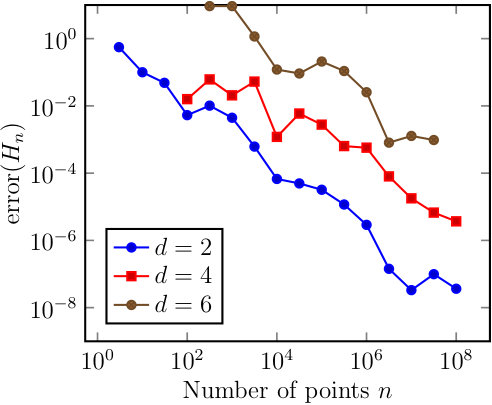 Figure 1
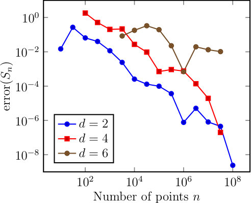 Figure 2
Peer Reviews
No public reviews on file for this paper yet. If you reviewed it on a platform where reviews are public (OpenReview, ICLR, NeurIPS, ICML), you can paste yours below so the community can read it here.
Videos
No videos yet. Explain this paper in a talk, walkthrough, or lecture? Add one.
Taxonomy
TopicsMathematical Approximation and Integration · Probabilistic and Robust Engineering Design · Statistical Methods and Inference
A weighted Discrepancy Bound of quasi-Monte Carlo Importance Sampling
Viacheslav Natarovskii, Daniel Rudolf, Björn Sprungk∗ Institute for Mathematical Stochastics, Georg-August-Universität Göttingen, Goldschmidtstraße 7, 37077 Göttingen, Email: [email protected], [email protected], [email protected] for Mathematical Statistics in the Biosciences, Goldschmidtstraße 7, 37077 Göttingen
Josef Dick, Daniel Rudolf, Houying Zhu The University of New South Wales, Sydney, NSW 2052, Australia, Email: [email protected] for Mathematical Stochastics, Universität Göttingen, Goldschmidtstraße 7, 37077 Göttingen, Germany, Email: [email protected] Integrative Genomics & School of Mathematics and Statistics, The University of Melbourne, Parkville, VIC 3010, Australia, Email: [email protected]
Abstract
Importance sampling Monte-Carlo methods are widely used for the approximation of expectations with respect to partially known probability measures. In this paper we study a deterministic version of such an estimator based on quasi-Monte Carlo. We obtain an explicit error bound in terms of the star-discrepancy for this method.
**Keywords: ** Importance sampling, Monte Carlo method, quasi-Monte Carlo
Classification. Primary: 62F15; Secondary: 11K45.
1 Introduction
In statistical physics and Bayesian statistics it is desirable to compute expected values
[TABLE]
with and a partially known probability measure on . Here denotes the Borel -algebra and partially known means that there is an unnormalized density (with respect to the Lebesgue measure) and , such that
[TABLE]
Probability measures of this type are met in numerous applications. For example, for the density of a Boltzmann distribution one has
[TABLE]
with inverse temperature and Hamiltonian . The density of a posterior distribution is also of this form. Given observations , likelihood function and prior probability density , with respect to the Lebesgue measure on ,
[TABLE]
In this setting is considered as parameter- and as observable-space. In both examples, the normalizing constant is in general unknown.
In the present work we only consider unnormalized densities which are zero outside of the unit cube . Hence we restrict ourself to , i.e., is a probability measure on , and . To stress the dependence on the unnormalized density in (1), define
[TABLE]
for and belonging to some class of functions. It is desirable to have algorithms which approximately compute by only having access to function values of and without knowing the normalizing constant a priori. A straightforward strategy to do so provides an importance sampling Monte Carlo approach. It works as follows.
Algorithm 1**.**
Monte Carlo importance sampling:
Generate a sample of an i.i.d. sequence of random variables with 111By we denote the uniform distribution on . and call the result . 2. 2.
Compute
[TABLE]
Under the minimal assumption that is finite, a strong law of large numbers argument guarantees that the importance sampling estimator is well-defined, cf. [16, Chapter 9, Theorem 9.2]. For uniformly bounded and finite an explicit error bound of the mean square error is proven in [14, Theorem 2].
Surprisingly, there is not much known about a deterministic version of this method. The idea is to substitute the uniformly in distributed i.i.d. sequence by a carefully chosen deterministic point set. Carefully chosen in the sense that the point set has “small” star-discrepancy, that is,
[TABLE]
is “small”. Here, the set denotes an anchored box in with and is the -dimensional Lebesgue measure of . This leads to a quasi-Monte Carlo importance sampling method.
Algorithm 2**.**
Quasi-Monte Carlo importance sampling:
Generate a point set with “small” star discrepancy . 2. 2.
Compute
[TABLE]
Our main result, stated in Theorem 3, is an explicit error bound for the estimator of the form
[TABLE]
Here must be differentiable, such that , defined in (7) below, is finite. As a regularity assumption on it is assumed that , defined in (9) below, is also finite.
The estimate of (4) is proven by two results which might be interesting on its own. The first is a Koksma-Hlawka inequality in terms of a weighted star-discrepancy, see Theorem 1. The second is a relation between this quantity and the classical star-discrepancy, see Theorem 2. To illustrate the quasi-Monte Carlo importance sampling procedure and the error bound we provide an example in Section 3 where (4) is applicable.
Related Literature. The Monte Carlo importance sampling procedure from Algorithm 1 is well studied. In [14], Novak and Mathé prove that it is optimal on a certain class of tuples . However, recently this Monte Carlo approach attracted considerable attention, let us mention here [1, 4]. In particular, in [1] upper error bounds not only for bounded functions are provided and the relevance of the method for inverse problems is presented.
Another standard approach the approximation of are Markov chain Monte Carlo methods. For details concerning error bounds we refer to [11, 12, 13, 17, 19, 20, 21] and the references therein. Combinations of importance sampling and Markov chain Monte Carlo are for example analyzed in [18, 24, 22].
The quasi-Monte Carlo importance sampling procedure of Algorithm 2 is, to our knowledge, less well studied. An asymptotic convergence result is stated in [9, Theorem 1] and promising numerical experiments are conducted in [10]. A related method, a randomized deterministic sampling procedure according to the unnormalized distribution , is studied in [23]. Recently, [3] explore the efficiency of using QMC inputs in importance sampling for Archimedean copulas where significant variance reduction is obtained for a case study.
A quasi-Monte Carlo approach to Bayesian inversion was used in [5] and in [6] The latter paper uses a combination of quasi-Monte Carlo and the multi-level method. The computation of the likelihood function involves solving a partial differential equation, but otherwise the problem is of the same form as described in the introduction.
2 Weighted Star-discrepancy and error bound
Recall that for are boxes anchored at [math]. As a measure of “closeness” between the empirical distribution of a point set to we consider the star-discrepancy . A straightforward extension of this quantity taking the probability measure on into account is the following weighted discrepancy.
Definition 1** (Weighted Star-discrepancy).**
For a given point set and weight vector , which might depend on and satisfies , define the weighted star-discrepancy by
[TABLE]
Remark 1**.**
If is the Lebesgue measure on and the weight vector is , then for any point set . For general with unnormalized density , allowing the representation (2), we focus on the weight vector
[TABLE]
Here let us emphasize that depends on and .
2.1 Integration Error and weighted Star-discrepancy
With standard techniques one can prove a Koksma-Hlawka inequality according to . For details we refer to [7], [8, Section 2.3] and [15, Chapter 9]. A similar inequality of a quasi-Monte Carlo importance sampler can be found in [2, Corollary 1].
Let and be the space of square integrable functions with respect to the Lebesgue measure. Define the reproducing kernel by By we denote the corresponding reproducing kernel Hilbert space, which consists of differentiable functions with respect to all variables with first partial derivatives being in . For the inner product is given by
[TABLE]
where for and we write and with if and if . Thus, consists of functions which are differentiable according to all variables with first partial derivatives being in . Note that, for holds
[TABLE]
where with . Thus, the reproducing property of the reproducing kernel Hilbert space can be rewritten as
[TABLE]
Further, we define the space of differentiable functions with finite norm
[TABLE]
where for we have . We also define the semi-norm
[TABLE]
It is obvious that .
We have the following relation between the integration error in and the weighted discrepancy.
Theorem 1** (Koskma-Hlawka inequality).**
Let be a probability measure of the form (2) with unnormalized density . Then, for , arbitrary weight vector with , and for all we have
[TABLE]
Proof.
Define the quadrature error of the approximation of by . Define the function . Then , and .
For
[TABLE]
and we have A straightforward calculation, see also for instance [7, formula (3)], shows by using (6) that
[TABLE]
Finally, by we have
[TABLE]
which finishes the proof. ∎
An immediate consequence of the theorem with from (5) and from (3) is the error bound
[TABLE]
Here the dependence on on the right-hand side is hidden in through and . The intuition is, that under suitable assumptions on the weighted star-discrepancy can be bounded by the classical star-discrepancy of .
2.2 Weighted and classical Star-discrepancy
In this section we provide a relation between the classical star-discrepancy and the weighted star-discrepancy .
Theorem 2**.**
Let be a probability measure of the form (2) with unnormalized density function . Then, for any point set in , we have
[TABLE]
where
[TABLE]
with and for .
Proof.
For the given point set and unnormalized density recall that is defined in (5). To shorten the notation define . Then, for we have
[TABLE]
For denote and let be the cardinality of . Define
[TABLE]
and note that
[TABLE]
Estimation of : An immediate consequence of the definition of is
[TABLE]
Estimation of : With the transformation defined in the theorem one has Let
[TABLE]
and observe that . Then
[TABLE]
where the last inequality follows from Theorem 1 with and constant unnormalized density. Further,
[TABLE]
By the fact that is again a box anchored at [math] and
[TABLE]
we have
[TABLE]
Hence we have
[TABLE]
which implies the result. ∎
In particular, the theorem implies that whenever is finite and goes to zero as goes to infinity, also goes to zero for increasing with the same rate of convergence.
2.3 Explicit error bound
An immediate consequence of the results of the previous two sections is the following explicit error bound of the quasi-Monte Carlo importance sampling method of Algorithm 2.
Theorem 3**.**
Let be a probability measure of the form (2) with unnormalized density . Then, for any point set in , and from (3) we obtain
[TABLE]
with from Theorem 2.
Under the regularity assumption that is finite, the error bound tells us that the classical star-discrepancy determines the rate of convergence on how fast goes to .
3 Illustrating Example
Define the -simplex by and consider the (slightly differently formulated) unnormalized density of the Dirichlet distribution with parameter vector given by
[TABLE]
The Dirichlet distribution is the conjugate prior of the multinomial distribution: Assume that we observed some data , which we model as a realization of a multinomial distributed random variable with unknown parameter vector . With this leads to a likelihood function For a prior distribution with unnormalized density and we obtain a posterior measure with unnormalized density .
The normalizing constant of can be computed explicitly, it is known that
[TABLE]
To have a feasible setting for the application of Theorem 1 and Theorem 2 we need to show that is finite. This is not immediately clear, since in we take the supremum over . The following lemma is useful.
Lemma 1**.**
Let and recall that we write . Define with if , if and if . Assume that for and . Then
[TABLE]
with
Proof.
The statement follows by induction over the cardinality of . For , i.e., both sides of (13) are equal to .
Assume , i.e., for some we have . Then
[TABLE]
with where the th entry is “1”. On the other hand
[TABLE]
By the fact that and the claim is proven for .
Now assume that (13) is true for any with . Let with be an arbitrary subset and let with . Then we prove that the result also holds for . We have
[TABLE]
Observe that
[TABLE]
where . Further, note that
[TABLE]
Hence, by using we obtain
[TABLE]
and the proof is finished. ∎
An immediate consequence of the previous lemma and a chain rule argument we have for arbitrary , and , defined as in Theorem 2, that
[TABLE]
For with , and arbitrary , holds , where , and . Then, it follows that with a constant depending on and . Hence, for another constant holds uniformly in . Finally, by the fact that we obtain the following corollary.
Corollary 1**.**
For with and we have for defined in (11) that there is a constant such that
[TABLE]
This verifies that the application of Theorem 1 and Theorem 2 is justified. For given by (5) we obtain
[TABLE]
Consider with given by Then, by (12) we have
[TABLE]
and . Since we know we can run the quasi-Monte Carlo importance sampling algorithm and plot the error for different and fixed and .
Numerical experiments. Let and . Here the true expectation of according to the distribution determined by can be further simplified to Since for large this value is very small we plot the normalized error. For a given point set it is defined by
[TABLE]
and can be computed exactly. Let the first points of the Halton sequence and note that it is known that . By we denote the first points of the Sobol sequence. For details to those standard quasi-Monte Carlo point sets we refer to [8]. We obtain the following plots for .
Acknowledgment
D. Rudolf is supported by the Felix-Bernstein-Institute for Mathematical Statistics in the Biosciences, the Campus laboratory AIMS and the DFG within the project 389483880.
The reference list from the paper itself. Each links out to its DOI / PubMed record.
- 1[1] S. Agapiou, O. Papaspiliopoulos, D. Sanz-Alonso, and A. Stuart, Importance Sampling: Intrinsic Dimension and Computational Cost , Statist. Sci. 32 .
- 2[2] Ch. Aistleitner and J. Dick, Functions of bounded variation, signed measures, and a general Koksma–Hlawka inequality , Acta Arith. 167 (2015), 143–171.
- 3[3] P. Arbenz, M. Cambou, M. Hofert, C. Lemieux, and Y. Taniguchi, Importance sampling and stratification for copula models , Contemporary Computational Mathematics - a celebration of the 80th birthday of Ian Sloan (J. Dick, F. Y. Kuo, H. Woźniakowski, eds.), Springer-Verlag, 2018.
- 4[4] S. Chatterjee and P Diaconis, The sample size required in importance sampling , Ann. Appl. Probab. 28 (2018), 1099–1135.
- 5[5] J. Dick, R. N. Gantner, Q. T. Le Gia, and C. Schwab, Higher order Quasi-Monte Carlo integration for Bayesian Estimation , Ar Xiv e-prints (2016).
- 6[6] , Multilevel higher-order quasi-Monte Carlo Bayesian estimation , Math. Models Methods Appl. Sci. 27 (2017), 953–995.
- 7[7] J. Dick, A. Hinrichs, and F. Pillichshammer, Proof Techniques in Quasi-Monte Carlo Theory , J. Complexity 31 (2015), 327–371.
- 8[8] J. Dick and F. Pillichshammer, Digital nets and sequences: Discrepancy theory and quasi-Monte Carlo integration , Cambridge University Press, Cambridge, 2010.