A general method to obtain the spectrum and local spectra of a graph from its regular partitions
C. Dalf\'o, M. A. Fiol

TL;DR
This paper introduces a comprehensive method to derive the entire spectrum and local spectra of a graph using quotient matrices from regular partitions, applicable to various classes like walk-regular and distance-regular graphs.
Contribution
It presents a new general approach to obtain all spectral information of a graph from its regular partitions, extending previous partial results.
Findings
Method successfully computes full spectra of various graph classes.
Applicable to walk-regular, distance-regular, and distance-biregular graphs.
Provides explicit eigenvalues and multiplicities from quotient matrices.
Abstract
It is well known that, in general, part of the spectrum of a graph can be obtained from the adjacency matrix of its quotient graph given by a regular partition. In this paper, we propose a method to obtain all the spectrum, and also the local spectra, of a graph from the quotient matrices of some of its regular partitions. As examples, it is shown how to find the eigenvalues and (local) multiplicities of walk-regular, distance-regular, and distance-biregular graphs.
Click any figure to enlarge with its caption.
 Figure 1
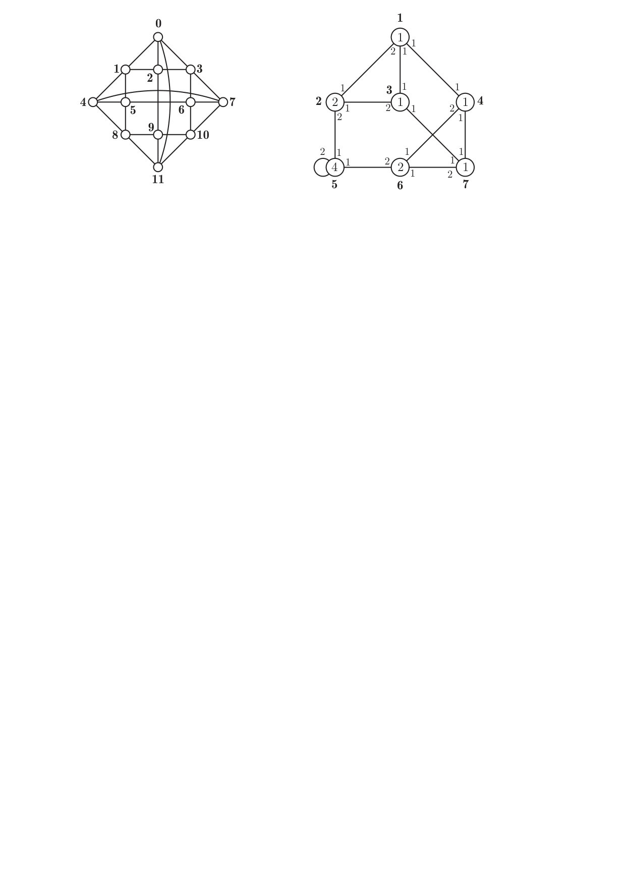 Figure 1
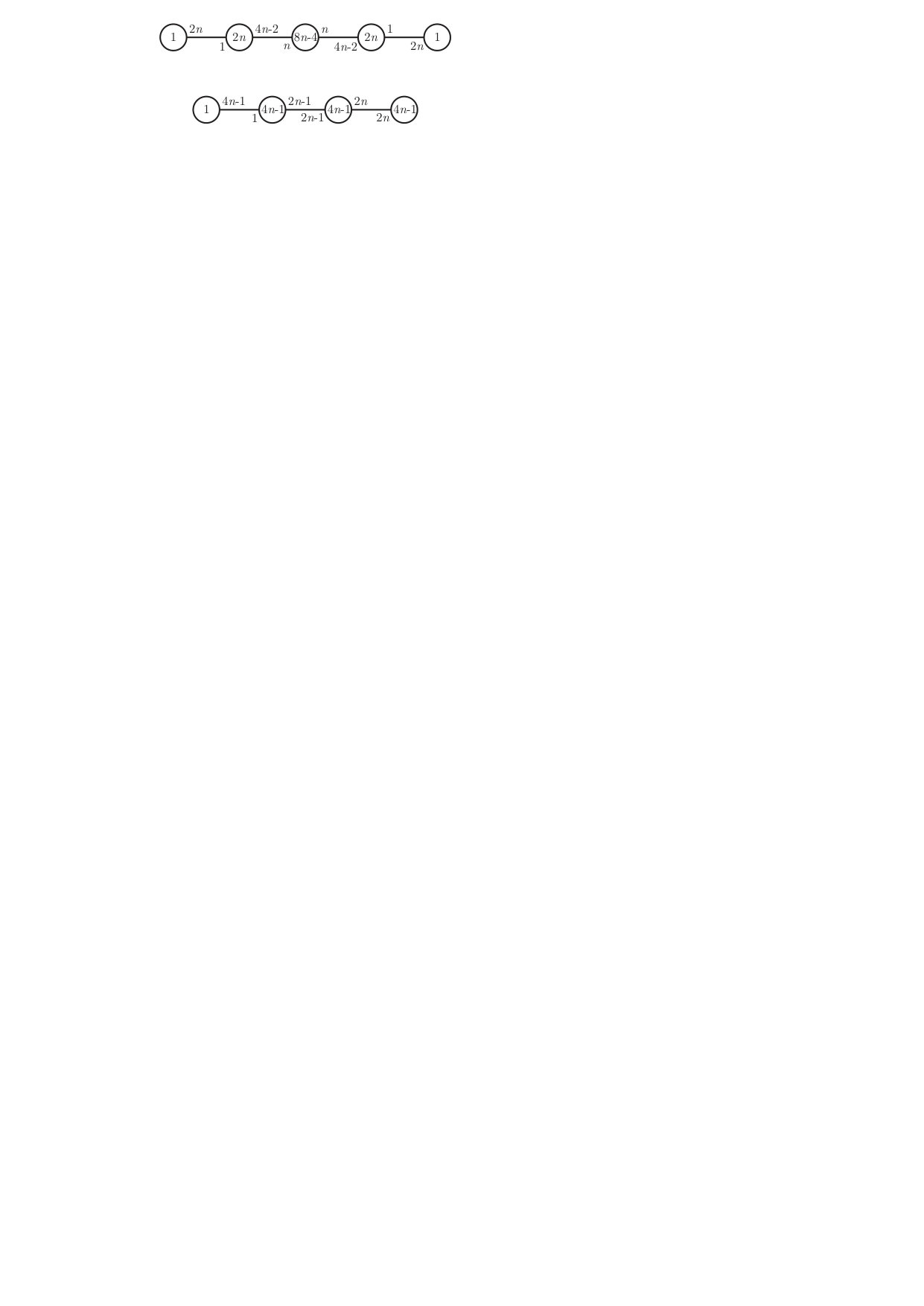 Figure 2
| , | 0 | 1 | 2 | 3 | 4 |
|---|---|---|---|---|---|
| , | 0 | 1 | 2 | 3 |
|---|---|---|---|---|
Peer Reviews
No public reviews on file for this paper yet. If you reviewed it on a platform where reviews are public (OpenReview, ICLR, NeurIPS, ICML), you can paste yours below so the community can read it here.
Videos
No videos yet. Explain this paper in a talk, walkthrough, or lecture? Add one.
Taxonomy
TopicsGraph theory and applications · Finite Group Theory Research · graph theory and CDMA systems
A general method to obtain the spectrum and
local spectra of a graph from its regular partitions ††thanks: This research is partially supported by the project 2017SGR1087 of the Agency for the Management of University and Research Grants (AGAUR) of the Government of Catalonia.
C. Dalfó
Departament de Matemàtica
Universitat de Lleida, Igualada (Barcelona), Catalonia
M. A. Fiol
Deptartament de Matemàtiques
Barcelona Graduate School of Mathematics,
Universitat Politècnica de Catalunya, Barcelona, Catalonia
Abstract
It is well known that, in general, part of the spectrum of a graph can be obtained from the adjacency matrix of its quotient graph given by a regular partition. In this paper, we propose a method to obtain all the spectrum, and also the local spectra, of a graph from the quotient matrices of some of its regular partitions. As examples, it is shown how to find the eigenvalues and (local) multiplicities of walk-regular, distance-regular, and distance-biregular graphs.
Keywords: Graph; Adjacency matrix; Spectrum; Eigenvalues; Local multiplicities; Walk-regular graph.
2010 Mathematics Subject Classification: 05E30, 05C50.
††
The first author has also received funding from the European Union’s Horizon 2020 research and innovation programme under the Marie Skłodowska-Curie grant agreement No 734922.
1 Preliminaries
First, let us recall some basic concepts and define our generic notation for graphs.
1.1 Some notions on graphs and their spectra
Throughout this paper, denotes a simple and connected graph with order , size , and adjacency matrix . The distance between two vertices and is denoted by , so that the eccentricity of a vertex is , and the diameter of the graph is . The set of vertices at distance , from a given vertex is denoted by , for , and we write for short. The degree of a vertex is denoted by . The distance- graph is the graph with vertex set , and where two vertices and are adjacent if and only if in . Its adjacency matrix {\mbox{\boldmathA}}_{i} is usually referred to as the distance- matrix of . The spectrum of a graph of its adjacency matrix {\mbox{\boldmathA}}(={\mbox{\boldmathA}}_{1}) is denoted by
[TABLE]
where the different eigenvalues of , whose set is denoted by , are in decreasing order, , and the superscripts stand for their multiplicities for . In particular, note that , since is connected, and . Alternatively, if we include repetitions, the eigenvalues of are denoted as
1.2 Projections and local spectra
For any graph with eigenvalue having multiplicity , its corresponding principal idempotent can be computed as {\mbox{\boldmathE}}_{i}=\mbox{\boldmathV}_{i}\mbox{\boldmathV}_{i}^{\top}, where \mbox{\boldmathV}_{i} is the matrix whose columns form an orthonormal basis of the eigenspace {\cal E}_{i}=\mathop{\rm Ker}\nolimits({\mbox{\boldmathA}}-\theta_{i}{\mbox{\boldmathI}}). For instance, when is a -regular graph on vertices, its largest eigenvalue has eigenvector , the all- (column) vector, and corresponding idempotent {\mbox{\boldmathE}}_{0}=\frac{1}{n}{\mbox{\boldmathj}}{\mbox{\boldmathj}}^{\top}=\frac{1}{n}{\mbox{\boldmathJ}}, where is the all- matrix.
Alternatively, for every , the orthogonal projection of onto the eigenspace is given by the Lagrange interpolating polynomial
[TABLE]
of degree , where . These polynomials satisfy and for . The idempotents are, then,
[TABLE]
and they are known to satisfy the following properties (see, for instance, Godsil [9, p. 28]):
{\mbox{\boldmathE}}_{i}{\mbox{\boldmathE}}_{j}=\delta_{ij}{\mbox{\boldmathE}}_{i};
{\mbox{\boldmathA}}{\mbox{\boldmathE}}_{i}=\theta_{i}{\mbox{\boldmathE}}_{i};
p({\mbox{\boldmathA}})=\displaystyle\sum_{i=0}^{d}p(\theta_{i}){\mbox{\boldmathE}}_{i}, for any polynomial .
In particular, when in , we have the so-called spectral decomposition theorem: {\mbox{\boldmathA}}=\sum_{i=0}^{d}\theta_{i}{\mbox{\boldmathE}}_{i}. The -local multiplicities of the eigenvalue , introduced by Fiol and Garriga in [7], were defined as the square norm of the projection of {\mbox{\boldmathe}}_{u} onto the eigenspace , where {\mbox{\boldmathe}}_{u} is the unitary characteristic vector of a vertex . That is,
[TABLE]
Notice that, in fact, , where is the angle between {\mbox{\boldmathe}}_{u} and {\mbox{\boldmathE}}_{i}{\mbox{\boldmathe}}_{u}. The values , for and , were formally introduced by Cvetković as the ‘angles’ of (see, for instance, Cvetković and Doob [2]).
The local multiplicities can be seen as a generalization of the (standard) multiplicities when the graph is ‘seen’ from the ‘base vertex’ . Indeed, they satisfy the following properties (see Fiol and Garriga [7]):
[TABLE]
If represent the eigenvalues of with non-null -local multiplicity, we define the -local spectrum of as
[TABLE]
By analogy with the local multiplicities, which correspond to the diagonal entries of the idempotents, Fiol, Garriga, and Yebra [8] defined the crossed -local multiplicities of the eigenvalue , denoted by , as
[TABLE]
(Thus, in particular, .) These parameters allow us to compute the number of walks of length between two vertices in the following way:
[TABLE]
Conversely, the values , for , determine the crossed local multiplicities . (Indeed, notice that the coefficients of the system in (4) are the entries of a Vandermonde matrix).
2 Regular partitions and local spectra
Let be a graph with adjacency matrix . A partition of its vertex set is called regular (or equitable) whenever, for any , the intersection numbers , where , do not depend on the vertex but only on the subsets (usually called classes or cells) and . In this case, such numbers are simply written as , and the matrix {\mbox{\boldmathB}}=(b_{ij}) is referred to as the quotient matrix of with respect to . This is also represented by the quotient (weighted) graph (associated to the partition ), with vertices representing the cells, and there is an edge with weight between vertex and vertex if and only if . Of course, if , for some , the quotient graph has loops.
The characteristic matrix of (any) partition is the matrix \mbox{\boldmathS}=(s_{ui}) whose -th column is the characteristic vector of , that is, if , and otherwise. In terms of this matrix, we have the following characterization of regular partitions (see Godsil [9]).
Lemma 2.1** ([9]).**
Let be a graph with adjacency matrix , and vertex partition with characteristic matrix . Then, is regular if and only if there exists an matrix such that \mbox{\boldmathS}{\mbox{\boldmathC}}={\mbox{\boldmathA}}\mbox{\boldmathS}. Moreover, {\mbox{\boldmathC}}={\mbox{\boldmathB}}, the quotient matrix of with respect to .
Using the above lemma, it can be proved that \mathop{\rm sp}\nolimits{\mbox{\boldmathB}}\subseteq\mathop{\rm sp}\nolimits{\mbox{\boldmathA}}. Moreover, we have the following result by the authors [3].
Lemma 2.2** ([3]).**
Let be a graph with adjacency matrix . Let be a regular partition of , with quotient matrix . Then, the number of -walks from any vertex to all vertices of is the -entry of {\mbox{\boldmathB}}^{\ell}.
By using the last lemma, now we have the next result.
Lemma 2.3**.**
Let be a graph with adjacency matrix , and a regular partition of with quotient matrix . If , then the number of -walks from vertex to a vertex , for , only depends on :
[TABLE]
Proof.
To prove that the number of -walks between and is a constant, we use induction on . The result is clearly true for , since {\mbox{\boldmathB}}^{0}={\mbox{\boldmathI}}, and for because of the definition of . Suppose that the result holds for some . Then, the set of walks of length from to is obtained from the set of -walks from to vertices adjacent to . Then, the number of these walks is
[TABLE]
as claimed. ∎
Let be a quotient (diagonalizable) matrix as above, with \mathop{\rm sp}\nolimits{\mbox{\boldmathB}}=\{\tau_{0}^{m(\tau_{0})},\tau_{1}^{m(\tau_{1})}, , and let {\mbox{\boldmathD}}=\mathop{\rm diag}\nolimits(\tau_{0},\tau_{1},\ldots,\tau_{e}). Let be the matrix that diagonalizes , that is, \mbox{\boldmathQ}^{-1}{\mbox{\boldmathB}}\mbox{\boldmathQ}={\mbox{\boldmathD}}. For , let \mbox{\boldmathV}_{i} be the matrix formed by the columns of corresponding to the right -eigenvectors of . Let \mbox{\boldmathU}_{i} be the matrix formed by the corresponding rows of \mbox{\boldmathQ}^{-1}, which are the left -eigenvectors of . Then, the -th idempotent of is \overline{{\mbox{\boldmathE}}}_{i}=\mbox{\boldmathV}_{i}\mbox{\boldmathU}_{i}. Moreover, \overline{{\mbox{\boldmathE}}}_{i} can be computed as in the case of the (symmetric) adjacency matrix by using the Lagrange interpolating polynomial satisfying :
[TABLE]
The above results yield a simple method to compute the local spectra of a vertex in a given regular partition or, more generally, the crossed multiplicities between and any other vertex . Besides, with the union of the local spectra (applying (3)) of the different classes of vertices according to their corresponding regular partitions (that is, we ‘hung’ the quotient graph from every one of the different classes of vertices), we obtain all the spectrum of the original graph. Thus, the main result is the following.
Theorem 2.4**.**
Let be a graph with adjacency matrix and set of different eigenvalues . Let be a regular partition of , with . Let be the quotient matrix of , with set of different eigenvalues \mathop{\rm ev}\nolimits{\mbox{\boldmathB}}=\{\tau_{0},\tau_{1},\ldots,\tau_{e}\}\subseteq\mathop{\rm ev}\nolimits\Gamma. Let and be the Lagrange interpolating polynomials satisfying for , and for , respectively. Let {\mbox{\boldmathE}}_{i}=L_{i}({\mbox{\boldmathA}}) and \overline{{\mbox{\boldmathE}}}_{i}=\overline{L}_{i}({\mbox{\boldmathB}}) be the corresponding idempotents. Then, for every vertex , the crossed -local multiplicity of is
[TABLE]
or, alternatively,
[TABLE]
Proof.
Let . Then, for every and , and using Lemma 2.3, we have
[TABLE]
which proves (6). To prove (9), note first that, by the spectral decomposition theorem, {\mbox{\boldmathB}}^{r}=\sum_{i=0}^{e}\tau_{i}^{r}\overline{{\mbox{\boldmathE}}}_{i}. Then, by Lemma 2.3, the numbers of -walks from to are
[TABLE]
which, as already commented, determine the local multiplicities because of the system of equations
[TABLE]
But a (the) solution of this system is obtained when the multiplicities , for , are given by (9), as claimed. ∎
In particular, notice that this result allows us to compute the -local spectrum of as
[TABLE]
where \tau_{i}\in\mathop{\rm ev}\nolimits{\mbox{\boldmathB}} and m_{u}(\tau_{i})=(\overline{{\mbox{\boldmathE}}}_{i})_{11}, for .
Let us show an example.
Example 1**.**
Let be the cone of a -regular graph on vertices, where the ‘new’ vertex is joined to all vertices of . Then, has a regular partition with quotient matrix
[TABLE]
and eigenvalues and . (Notice that the first expression can be rewritten as , in agreement with the results of Dalfó, Fiol, and Garriga [4].) Thus, the idempotents of turn out to be \overline{{\mbox{\boldmathE}}}_{0}=({\mbox{\boldmathB}}-\theta_{1}{\mbox{\boldmathI}})/(\theta_{0}-\theta_{1}) and \overline{{\mbox{\boldmathE}}}_{1}=({\mbox{\boldmathB}}-\theta_{0}{\mbox{\boldmathI}})/(\theta_{1}-\theta_{0}). Consequently, Theorem 2.4 implies that the local -spectrum of is
[TABLE]
where and .
Another simple consequence of our main result is obtained for simple eigenvalues of .
Corollary 2.5**.**
Let be a graph with adjacency matrix and a set of different eigenvalues , a regular partition of with , the quotient matrix of with a set of different eigenvalues \mathop{\rm ev}\nolimits{\mbox{\boldmathB}}=\{\tau_{0},\tau_{1},\ldots,\tau_{e}\}\subseteq\mathop{\rm ev}\nolimits\Gamma, and {\mbox{\boldmathE}}_{i} and \overline{{\mbox{\boldmathE}}}_{i} the corresponding idempotents. Suppose that, for some , \theta_{i}\in\mathop{\rm ev}\nolimits{\mbox{\boldmathA}}\cap\mathop{\rm ev}\nolimits{\mbox{\boldmathB}} has multiplicity . Let {\mbox{\boldmathu}}_{i}=(u_{i1},\ldots,u_{im}) and {\mbox{\boldmathv}}_{i}=(v_{1i},\ldots,v_{im})^{\top} be the left and right eigenvectors of , respectively, corresponding to the eigenvalue . Then, for every vertex , the crossed -local multiplicity of in is
[TABLE]
Proof.
Let be a matrix that diagonalizes . If, for some constants and , we have that \alpha{\mbox{\boldmathu}}_{i} and \beta{\mbox{\boldmathv}}_{i} are the corresponding row of \mbox{\boldmathQ}^{-1} and column of , respectively, then (\mbox{\boldmathQ}^{-1}\mbox{\boldmathQ})_{ii}=1 implies that \alpha\beta=\langle{\mbox{\boldmathu}}_{i},{\mbox{\boldmathv}}_{i}\rangle^{-1}. Thus, (\overline{{\mbox{\boldmathE}}}_{i})_{1j}=(\alpha{\mbox{\boldmathv}}_{i}\cdot\beta{\mbox{\boldmathu}}_{i})_{1j}=\frac{v_{1i}u_{ij}}{\langle{\mbox{\boldmathu}}_{i},{\mbox{\boldmathv}}_{i}\rangle} (where ‘’ stands for the matrix product), and the result follows from (9). ∎
Alternatively, if {\mbox{\boldmathu}}_{i} and {\mbox{\boldmathv}}_{i} are already taken from the corresponding row and column of \mbox{\boldmathQ}^{-1} and , respectively, then , and (11) can be simply written as
[TABLE]
3 The local spectra of some families of graphs
In this last section, we show the application of our method to obtain the local spectra and the complete spectrum of different well-known families of graphs.
3.1 Walk-regular graphs
Let be a graph with spectrum as above. If the number of closed walks of length rooted at vertex , that is, only depends on , for each , then is called walk-regular (a concept introduced by Godsil and McKay [10]). In this case, we write . Note that, since , the degree of vertex , a walk-regular graph is necessarily regular. Moreover, we say that is spectrum-regular if, for any , the -local multiplicity of does not depend on the vertex . By (4) and the subsequent comment, it follows that spectrum-regularity and walk-regularity are equivalent concepts. Equation (4) also shows that the existence of the constants suffices to assure walk-regularity. It is well known that any distance-regular graph, as well as any vertex-transitive graph, is walk-regular, but the converse is not true.
Proposition 3.1**.**
Let be a walk-regular graph with vertices, having a regular partition with and quotient matrix . Then, the spectrum of is
[TABLE]
where, for every , also is an eigenvalue of , with multiplicity
[TABLE]
Proof.
Since , the (standard) multiplicity ‘splits’ equitably among the vertices, giving . Therefore, the different eigenvalues of coincide with those of , and Theorem 2.4 yields (13). ∎
Let us see an example.
Example 2**.**
Consider the walk-regular graph , that is not distance-regular, given by Godsil [9]. This graph and its quotient are represented in Figure 1. The spectrum of is . Since is walk-regular, the spectrum of its quotient from a regular partition has all the different eigenvalues of the spectrum of . Now we compute the multiplicities , for .
[TABLE]
This gives that the spectrum of is , as it is known to be. Note that, in this example, we need to ‘hang’ the graph from only one of its vertices.
3.2 Distance-regular graphs
In particular, when is distance-regular, the distance-partition with respect to any vertex is regular with the same quotient matrix (see, for instance, Biggs [1] or Fiol [6]). Moreover, since is tridiagonal, all its eigenvalues are simple and (13), together with (11), leads to the known formula (see Biggs [1])
[TABLE]
where the eigenvectors {\mbox{\boldmathu}}_{i} and {\mbox{\boldmathv}}_{i} have been chosen to have the first entry .
3.3 Distance-biregular graphs
Distance-biregular graphs are defined in a similar way as distance-regular graphs. They are connected bipartite graphs in which each of the two classes of vertices has its own intersection array. It was proved by Godsil and Shawe-Taylor [11] that all vertices in the same bipartition class have the same intersection array. Delorme [5] gave the basic properties and some new examples of distance-biregular graphs.
Let us give an example.
Example 3**.**
A Hadamard matrix (with entries and mutually orthogonal rows) with size gives a bipartite distance-biregular graph on vertices (see, for instance, Wallis [12, p. 426]). Its stable sets and have and vertices, respectively. For instance, is the subdivided complete graph . The quotient graphs corresponding to the regular distance-partitions with respect to vertices in and are shown in Figure 2. Thus, the respective quotient matrices are
[TABLE]
with (simple) eigenvalues \mathop{\rm ev}\nolimits{\mbox{\boldmathB}}_{1}=\{\sqrt{8n^{2}-1},\sqrt{2n},0,-\sqrt{2n},-\sqrt{8n^{2}-1}\} and \mathop{\rm ev}\nolimits{\mbox{\boldmathB}}_{2}=\mathop{\rm ev}\nolimits{\mbox{\boldmathB}}_{1}\setminus\{0\}. Then, according to Theorem 2.4, we can compute all the local (crossed) multiplicities of vertices in each stable set from the idempotents of {\mbox{\boldmathB}}_{1} and {\mbox{\boldmathB}}_{2}. The results obtained are shown in Table 1 (for ) and Table 2 (for ), where the last row in both tables corresponds to the sums in (4) for (or, for the case , to (2)). Moreover, from the columns of local multiplicities (), we can find the (global) multiplicities by using (3), which in our case becomes
[TABLE]
Then, the complete spectrum of the Hadamard distance-biregular graph turns out to be
[TABLE]
The reference list from the paper itself. Each links out to its DOI / PubMed record.
- 1[1] N. Biggs, Algebraic Graph Theory , Cambridge University Press, Cambridge, 1974, second edition, 1993.
- 2[2] D. M. Cvetković and M. Doob, Developments in the theory of graph spectra, Linear Multilinear Algebra 18 (1985) 153–181.
- 3[3] C. Dalfó and M. A. Fiol, A note on the order of iterated line digraphs, J. Graph Theory 85 (2017), no. 2, 395–399.
- 4[4] C. Dalfó, M. A. Fiol, and E. Garriga, A differential approach for bounding the index of graphs under perturbations, Electron. J. Combin. 18 (2011) #P 172.
- 5[5] C. Delorme, Distance biregular bipartite graphs, European J. Combin. 15 (1994) 223–238.
- 6[6] M. A. Fiol, Algebraic characterizations of distance-regular graphs, Discrete Math. 246 (2002) 111–129.
- 7[7] M. A. Fiol and E. Garriga, From local adjacency polynomials to locally pseudo-distance-regular graphs, J. Combin. Theory Ser. B 71 (1997) 162–183.
- 8[8] M. A. Fiol, E. Garriga, and J. L. A. Yebra, Boundary graphs: The limit case of a spectral property, Discrete Math. 226 (2001) 155–173.