Incremental Principal Component Analysis Exact implementation and continuity corrections
Vittorio Lippi, Giacomo Ceccarelli

TL;DR
This paper presents an exact incremental PCA algorithm that updates transformation coefficients in real-time without storing all data, ensuring continuity of principal components during online analysis.
Contribution
It introduces a formally equivalent incremental PCA method with continuity corrections, enabling real-time data analysis without batch processing.
Findings
The incremental PCA produces identical results to batch PCA.
The method maintains PC continuity during online updates.
Applications demonstrate real-time data analysis benefits.
Abstract
This paper describes some applications of an incremental implementation of the principal component analysis (PCA). The algorithm updates the transformation coefficients matrix on-line for each new sample, without the need to keep all the samples in memory. The algorithm is formally equivalent to the usual batch version, in the sense that given a sample set the transformation coefficients at the end of the process are the same. The implications of applying the PCA in real time are discussed with the help of data analysis examples. In particular we focus on the problem of the continuity of the PCs during an on-line analysis.
Click any figure to enlarge with its caption.
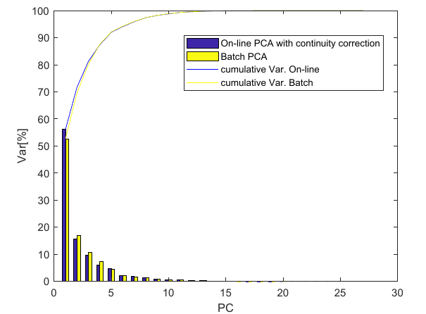 Figure 1
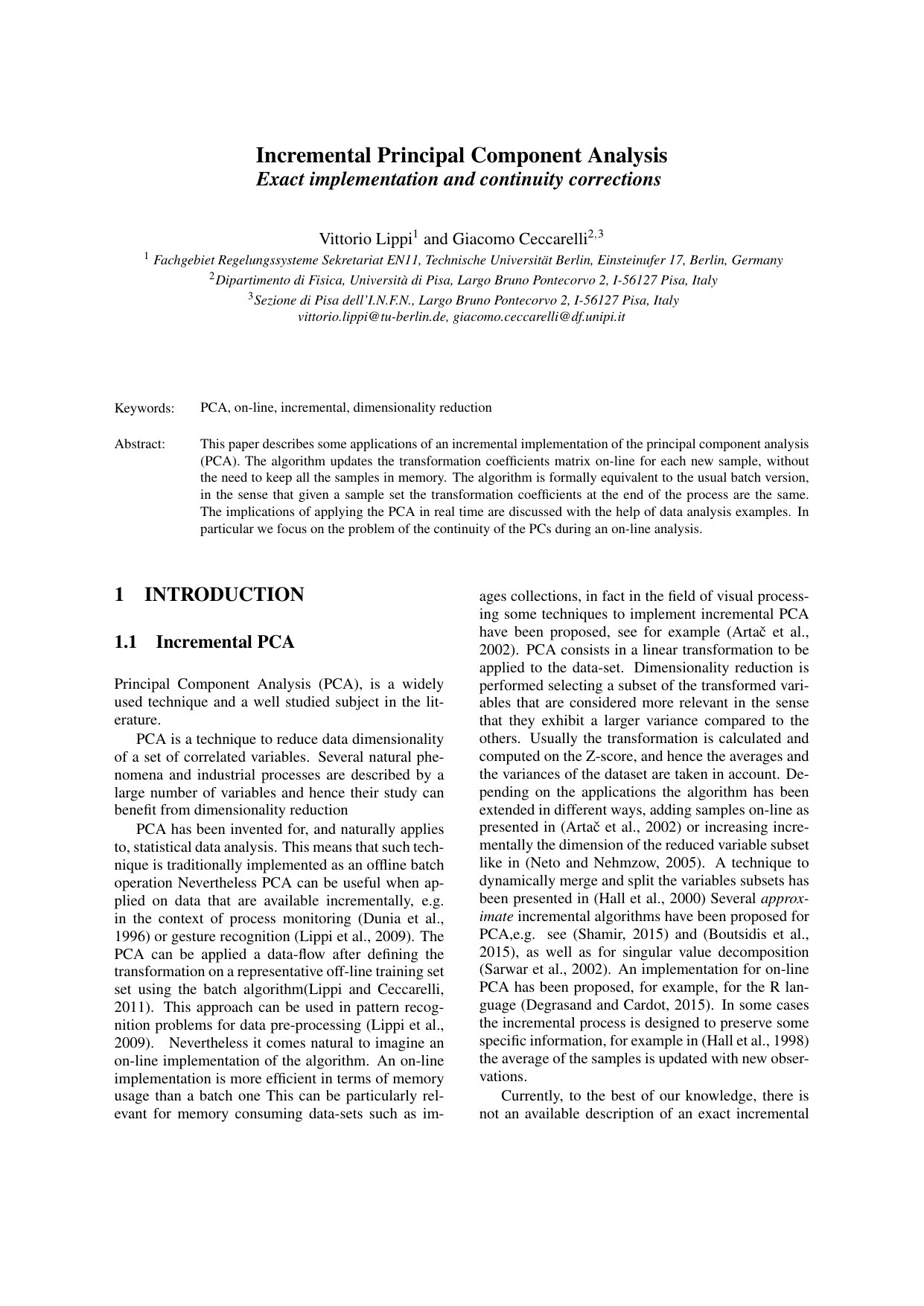 Figure 2
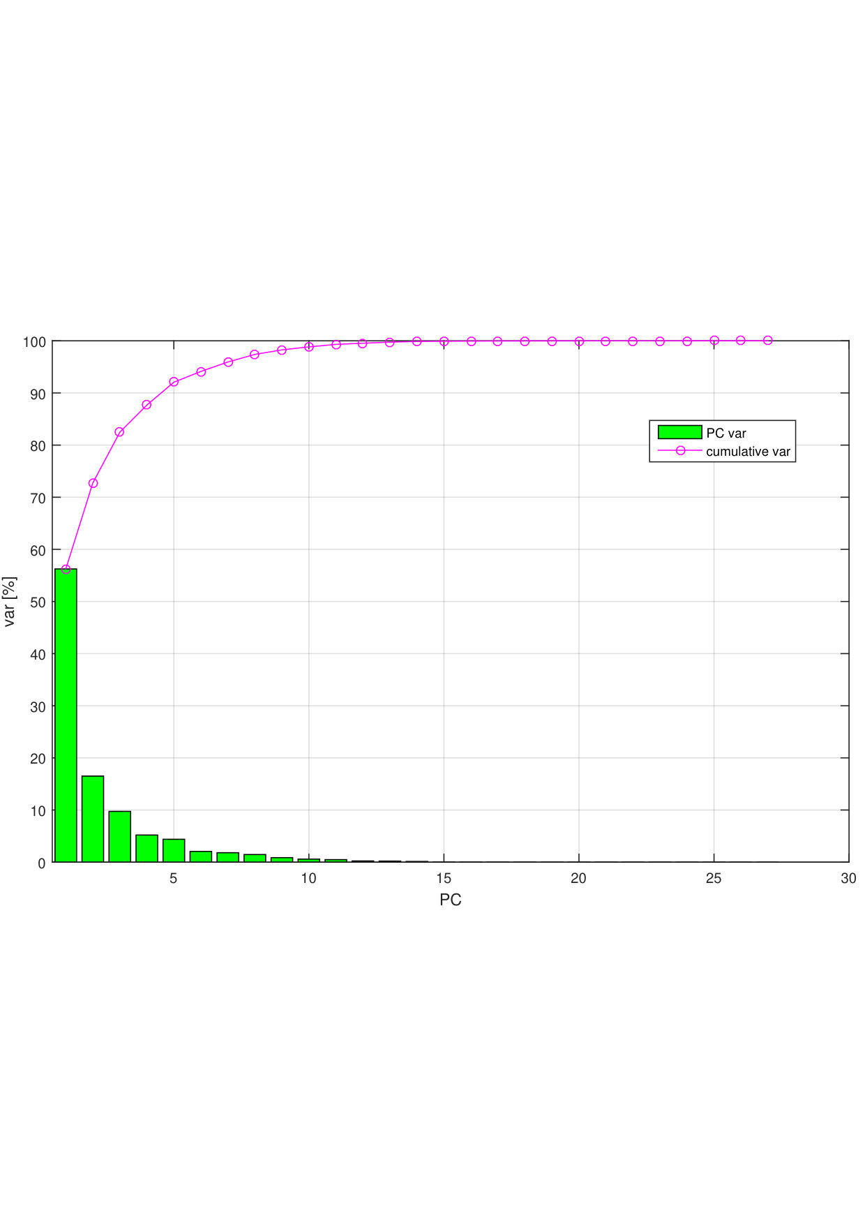 Figure 3
 Figure 4
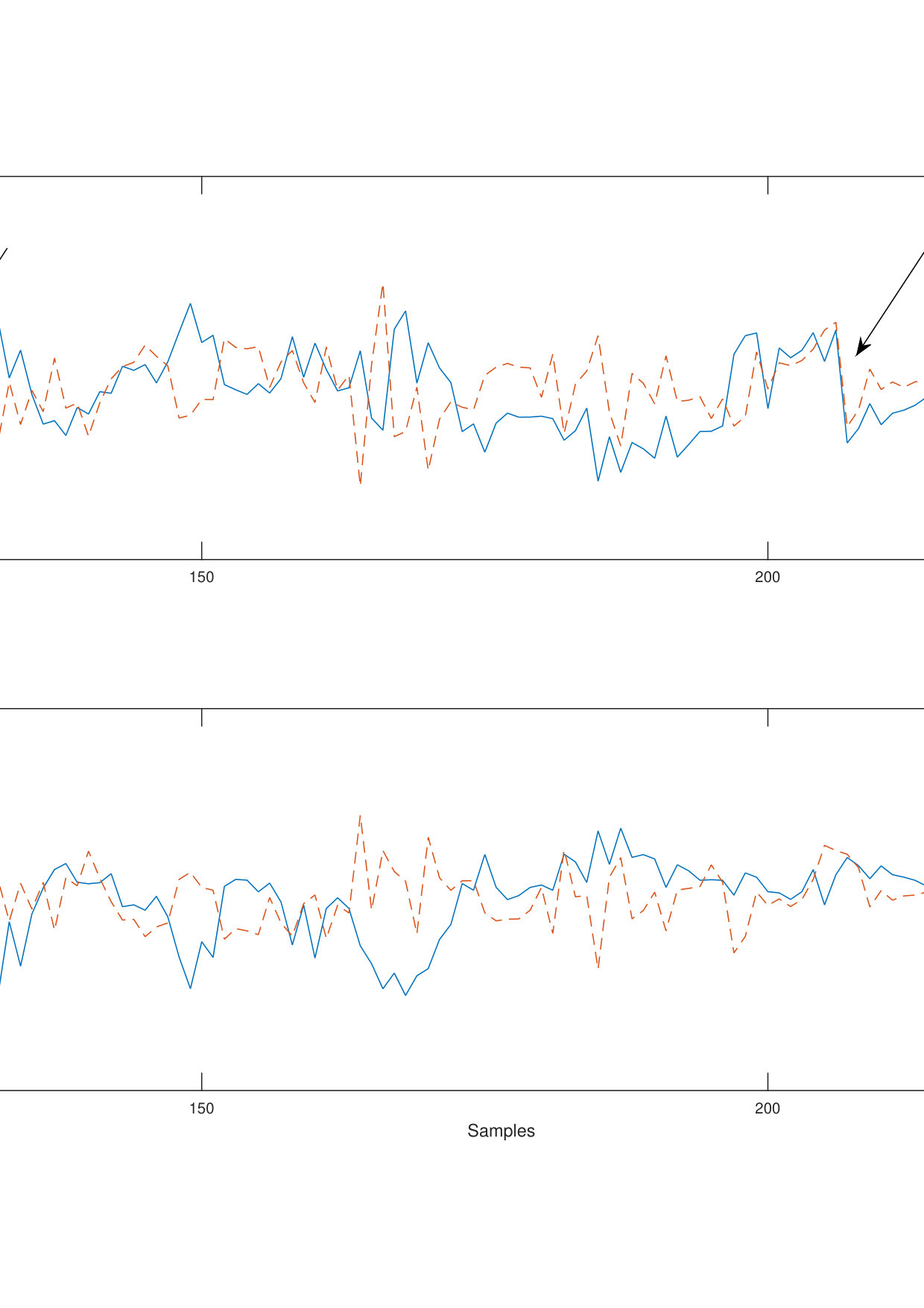 Figure 5
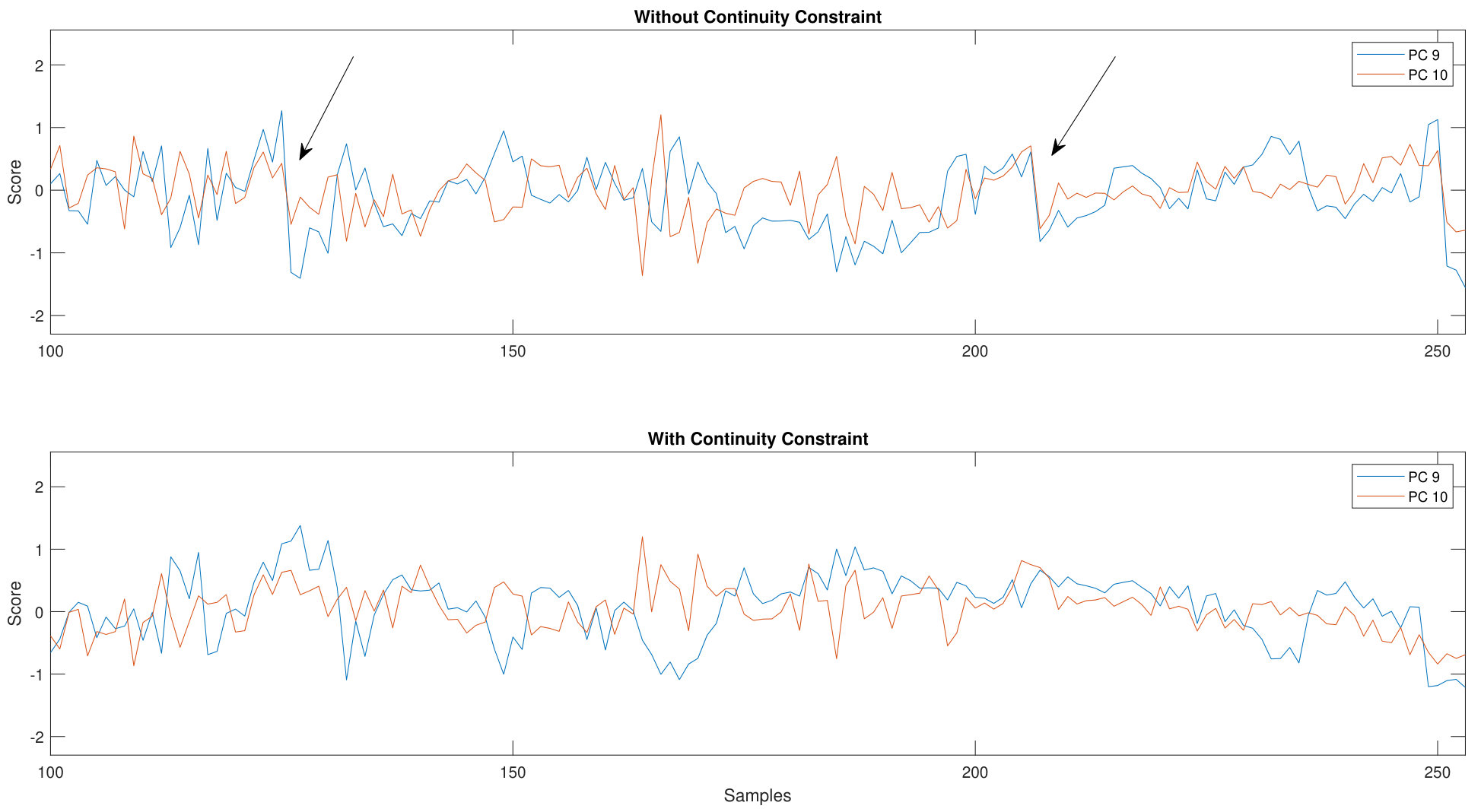 Figure 6
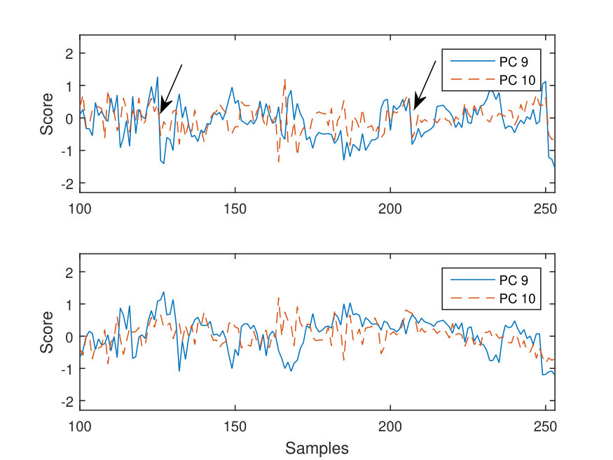 Figure 7
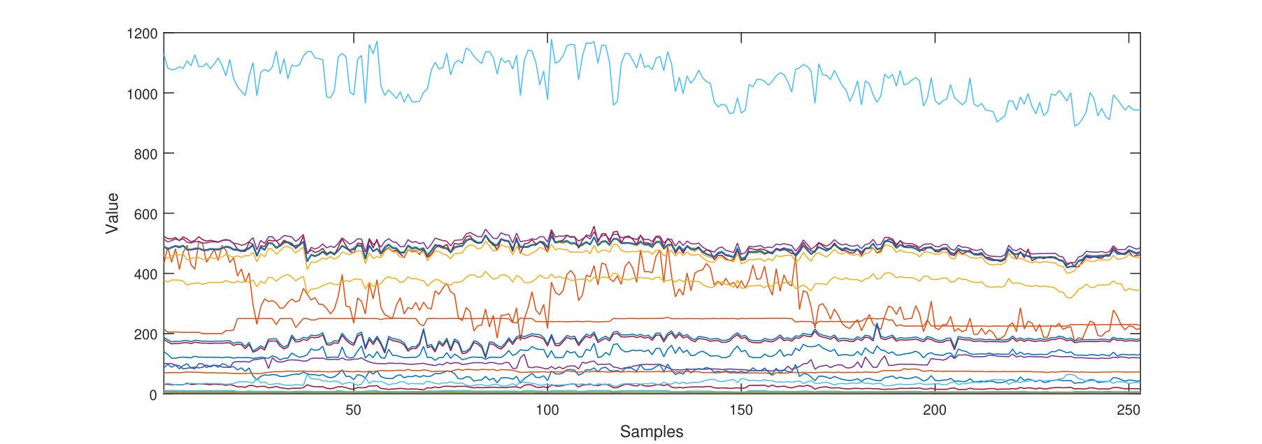 Figure 8
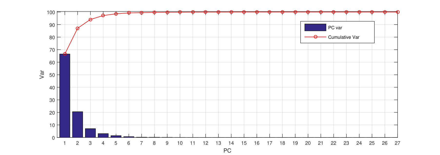 Figure 9
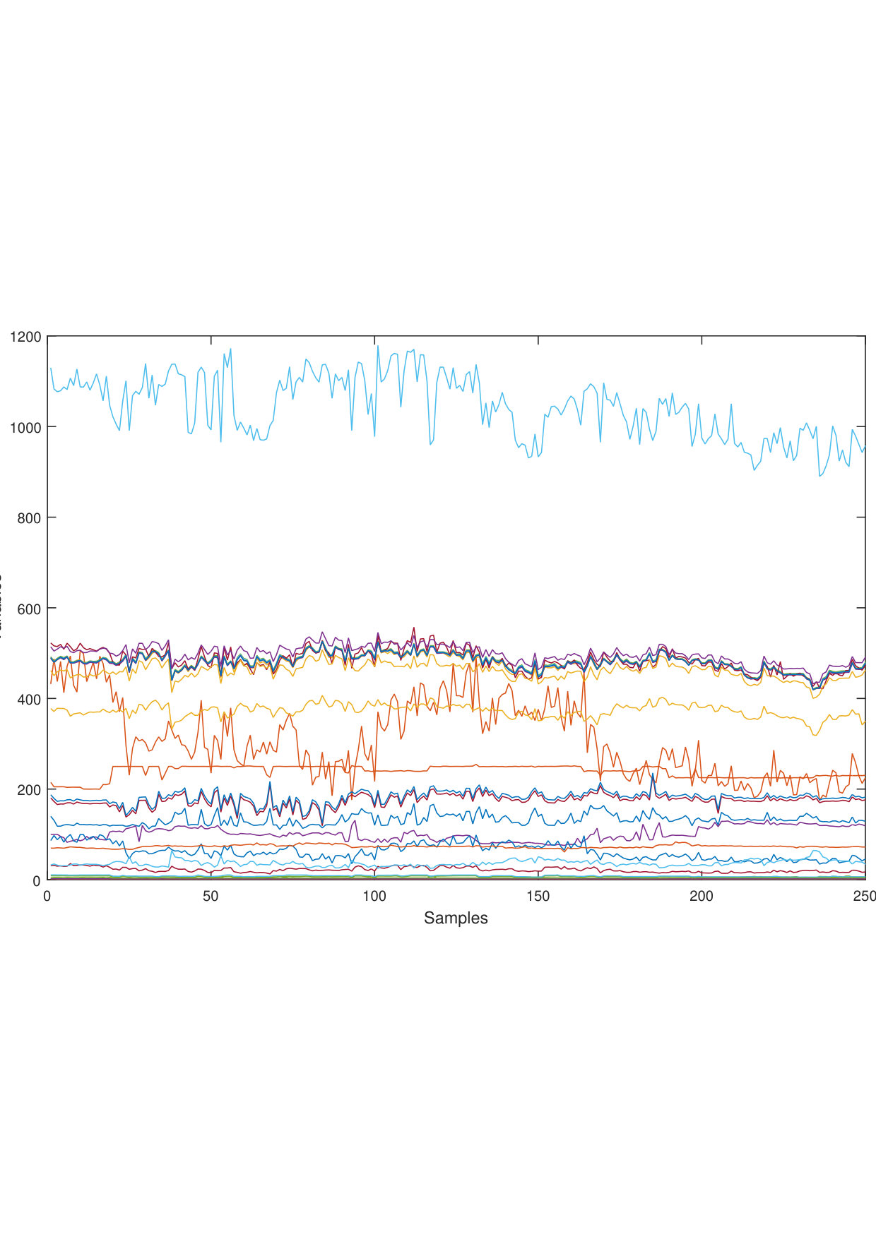 Figure 10
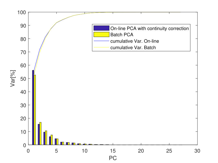 Figure 11
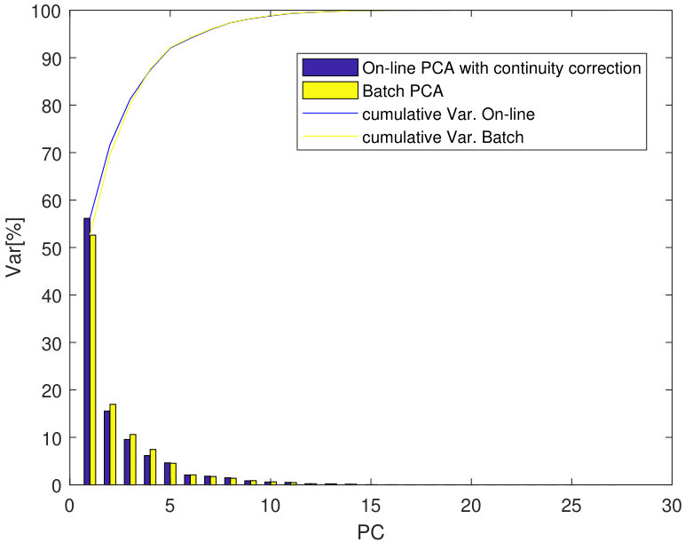 Figure 12
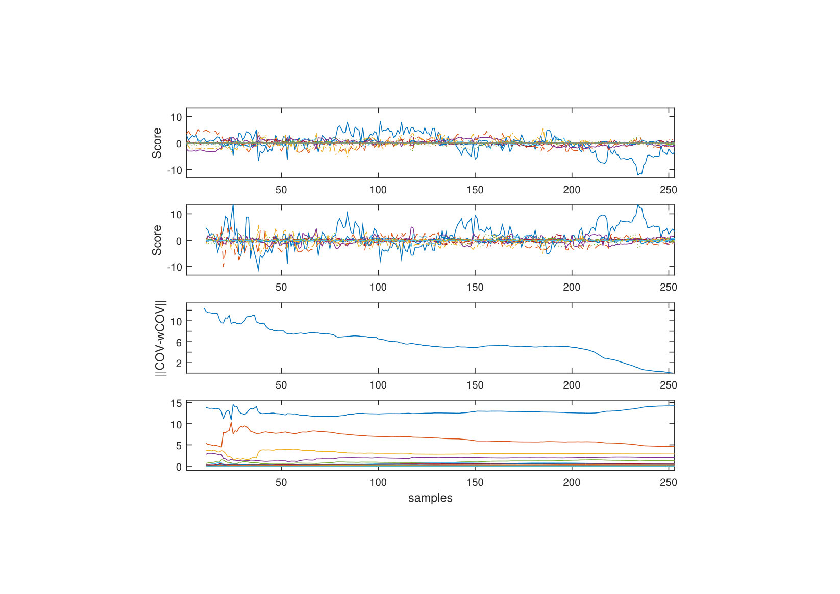 Figure 13
Peer Reviews
No public reviews on file for this paper yet. If you reviewed it on a platform where reviews are public (OpenReview, ICLR, NeurIPS, ICML), you can paste yours below so the community can read it here.
Videos
No videos yet. Explain this paper in a talk, walkthrough, or lecture? Add one.
Taxonomy
MethodsPrincipal Components Analysis
Incremental Principal Component Analysis
*Exact implementation and continuity corrections *
Vittorio Lippi1 and Giacomo Ceccarelli2
1* Fachgebiet Regelungssysteme Sekretariat EN11, Technische Universität Berlin, Einsteinufer 17, Berlin, Germany*
2**Dipartimento di Fisica, Università di Pisa, Largo Bruno Pontecorvo 2, I-56127 Pisa, Italy
[email protected], [email protected]
Abstract
This paper describes some applications of an incremental implementation of the principal component analysis (PCA). The algorithm updates the transformation coefficients matrix on-line for each new sample, without the need to keep all the samples in memory. The algorithm is formally equivalent to the usual batch version, in the sense that given a sample set the transformation coefficients at the end of the process are the same. The implications of applying the PCA in real time are discussed with the help of data analysis examples. In particular we focus on the problem of the continuity of the PCs during an on-line analysis.
1 INTRODUCTION
1.1 Incremental PCA
Principal Component Analysis (PCA) is a widely used technique and a well-studied subject in the literature. PCA is a technique to reduce data dimensionality of a set of correlated variables. Several natural phenomena and industrial processes are described by a large number of variables and hence their study can benefit from the dimensionality reduction PCA has been invented for. As such PCA naturally applies to statistical data analysis. This means that such technique is traditionally implemented as an offline batch operation. Nevertheless, PCA can be useful when applied to data that are available incrementally, e.g. in the context of process monitoring [Dunia et al., 1996] or gesture recognition [Lippi et al., 2009]. The PCA can be applied to a data-flow after defining the transformation on a representative off-line training set set using the batch algorithm [Lippi and Ceccarelli, 2011]. This approach can be used in pattern recognition problems for data pre-processing [Lippi et al., 2009]. Nevertheless one can imagine an on-line implementation of the algorithm. An on-line implementation is more efficient in terms of memory usage than a batch one. This can be particularly relevant for memory consuming data-sets such as image collections; in fact in the field of visual processing some techniques to implement incremental PCA have been proposed, see for example [Artač et al., 2002]. PCA consists of a linear transformation to be applied to the data-set. Dimensionality reduction is performed by selecting a subset of the transformed variables that are considered more relevant in the sense that they exhibit a larger variance compared to the others. Usually the transformation is calculated and computed on the Z-score, and hence the averages and the variances of the dataset are taken into account. Depending on the applications the algorithm has been extended in different ways, adding samples on-line as presented in [Artač et al., 2002] or incrementally increasing the dimension of the reduced variable subset as seen in [Neto and Nehmzow, 2005]. A technique to dynamically merge and split the variable subsets has been presented in [Hall et al., 2000] Several approximate incremental algorithms have been proposed for PCA, e.g. see [Shamir, 2015] and [Boutsidis et al., 2015], as well as for singular value decomposition [Sarwar et al., 2002]. An implementation for on-line PCA has been proposed, for example, for the R language [Degrasand and Cardot, 2015]. In some cases the incremental process is designed to preserve some specific information; for example in [Hall et al., 1998] the average of the samples is updated with new observations.
Currently, to the best of our knowledge, there is no available description of an exact incremental implementation of PCA, where exact means that the transformation obtained given samples is exactly the same as would have been produced by the batch algorithm, including the z-score normalization, a step that is not included in previous works presenting a similar approach like[Artač et al., 2002]. We decided in light of this to describe the algorithm in detail in this paper. The incremental techniques cited above [Hall et al., 1998, Artač et al., 2002, Hall et al., 2000] are designed to update the reduced set of variables and change its dimensionality when it is convenient for data representation. In the present work, no indication is provided for which subset of variables should be used , i.e. how many principal components to consider. All the components are used during the algorithm to ensure the exact solution. After describing the exact algorithm some implication of using this incremental analysis are discussed. In particular, we provide an intuitive definition of continuity for the obtained transformation and then we propose a modified version designed to avoid discontinuities.
The concept of continuity is strictly related to the incremental nature of the proposed algorithm: in standard PCA the batch analysis implies that the notion of time does not exist, e.g. the order of the elements in the sample set is not relevant for the batch algorithm. In our treatment we instead want to follow the time evolution of variances and eigenvectors. We are thus lead to consider a dynamical evolution.
The paper is organized as follows. In the remaining part of the Introduction we recall the PCA algorithm and we introduce the notation used. In Section 2.1 we give a detailed account of the incremental algorithm for an on-line use of PCA. In Section 2.2 we address the problems related to the data reconstruction, in particular those connected with the signal continuity. In Sections 3, 4 we then present the results of some applications to an industrial data set and draw our conclusions.
1.2 The principal component analysis
The computation for the PCA starts considering a set of observed data. We suppose we have sensors which sample some physical observables at constant rate. After observations we can construct the matrix
[TABLE]
where is a row vector of length representing the measurements of the time step so that is a real matrix whose columns represent all the values of a given observable.
The next step is to define the sample means and standard deviations with respect to the columns (i.e. for the observables) in the usual way as
[TABLE]
where in parentheses we write the matrix and vector indices explicitly. In this way we can define the standardized matrix for the data as
[TABLE]
where is a matrix. The covariance matrix of the data matrix is then defined as
[TABLE]
We see that is for any a symmetric matrix and it is positive definite.
Finally we make a standard diagonalization so that we can write
[TABLE]
where the (positive) eigenvalues are in descending order: . The transformation matrix is the eigenvectors matrix and it is orthogonal, . Its rows are the principal components of the matrix and the value of represents the variance associated to the principal component. Setting , we have a time evolution for the values of the PCs until time step .
We recall that the diagonalization procedure is not uniquely defined: once the order of the eigenvalues is chosen, one can still choose the “sign” of the eigenvector for one-dimensional eigenspaces and a suitable orthonormal basis for degenerate ones (in Section 2.2 we will see some consequences of this fact). We stress that, since only the eigenspace structure is an intrinsic property of the data, the PCs are quantity useful for their interpretation but they are not uniquely defined.
2 On-line analysis
2.1 Incremental algorithm
The aim of the algorithm is to construct the covariance matrix starting from the old matrix and the new observed data . To do this, at the beginning of step , we consider the sums of the observables and their squares after step :
[TABLE]
[TABLE]
These sums are updated on-line at every step. From these quantities we can recover the starting means and standard deviations: and . Similarly the current means and standard deviations are also simply obtained.
The key observation to get an incremental algorithm is the following identity:
[TABLE]
where is a row vector and is a matrix built repeating times the row vector . By definition and, expanding the preceding identity, we get
[TABLE]
where and we used the fact that the s are diagonal.
Recalling that by hypothesis all the columns of the matrix have zero mean and that the columns of the matrix have the same number, we see that terms in parentheses are zero. Thus
[TABLE]
where , and are three matrices. We now see that we can compute by making operations only on matrices and with the sole knowledge of and .
The computational advantage of this strategy is that we do not need to save in the memory all the sampled data and moreover we do not need to perform the explicit matrix product in eq. (5), which would require a great amount of memory and time for . Consequently this algorithm can be fruitfully applied in situations where the sensors number is small (e.g. of the order of tens) but the data stream is expected to grow quickly.
The meaning of the normalization procedure depends on the process under analysis and the meaning that is associated to the data within the current study: both centering around the empirical mean and dividing by the empirical variance can be avoided by respectively setting or .
In practice, one keeps observations and compute as given by eq. (5) and the relative (and hence ). Then the updated s are used, step by step, to compute the values for the evolving PCs in the standard way as . In this way the last sample is equal for any to the one that would result from a batch analysis until time step . Instead the whole sequence of the values with would not coincide with those from , since the s matrices change every time a sample is added, and likewise for the s matrices. The most relevant implications of this fact will be considered in the next subsection.
The library for the present implementation of the algorithm is available on the Mathworks website under the name incremental PCA.
2.2 Continuity issues
We now consider the problem of the continuity for the PCs during the on-line analysis. In a batch analysis, one computes the PCs using all the data at the end of the sampling, obtaining the matrix , and then, by applying this transformation and its inverse, one can pass from the original data set to the set PCs values. Of course, since we are considering sampled data, we cannot speak of continuity in a strict sense. As previously stated, the temporal evolution of the data is not something relevant for the batch PCA. Regardless, we may intuitively expect to use a sampling rate of at least two times the signal bandwidth (for the sampling theorem) usually even more, i.e. ten times. We hence expect a limited difference between two samples in proportion to the overall signal amplitude. For sampled data we can then define continuity in a intuitive sense as a condition where the difference between two consecutive samples is smaller than a given threshold. A discontinuity in the original samples may be reflected in the principal components depending on the transformation coefficients, in detail
[TABLE]
that is equal to
[TABLE]
The first term would be the same for the batch procedure (in that case with constant ) and the second term shows how is changing due to the change in coefficients . We can regard this term as the source of discontinuities due to the incremental algorithm.
To understand the problems that could arise, from the point of view of the continuity of the PCs values, let us consider the on-line procedure more closely.
We start with some the matrices and . At a numerical level the eigenvalues are all different (since the machine precision is at least of order ), so that we have a set of formally one-dimensional eigenspaces, from which the eigenvectors are taken. Going on in the time sampling, we naturally create different time series of eigenvectors.
We could expect that the difference of two subsequent eigenvectors of a given series be slowly varying (in the sense of the standard euclidean norm), since they come from different s that are obtained from different which differ only slightly (i.e. for the last ). But this is not fully justified, since the PCs are not uniquely defined and in some case two subsequent vectors of and can differ considerably, as shown in the exaple in Figure 4. There are three ways in which one or more eigenvector series could exhibit a discontinuity (in the general sense discussed above).
- •
Consider the case of a given eigenvalue associated with two eigenspaces at two subsequent time steps, spanned by the vectors and . They belong by hypothesis to two close “lines” but the algorithm can choose in the “wrong” direction. In this case, to preserve the on-line continuity as much as possible, we take the new PC to be , i.e. minus the eigenvector given by the diagonalization process at step . The “right” orientation can be identified with simple considerations on the scalar product of with . Recalling the considerations at the end of Section 1.2, this substitution does not change the meaning of our analysis.
- •
Consider the case where the differences of a group of contiguous eigenvalues are much smaller than the others: we can say that these eigenvalues correspond in fact to a degenerate eigenspace. In this case we can choose an infinite number of orthonormal vectors that can be legitimately considered our PCs, but the incremental algorithm can choose, at subsequent time steps, two basis which considerably differ. To overcome this problem, we must apply to the new transformation a change of basis in such a way not to modify the eigenspaces structure and to “minimize” the distance with the old basis. Although the case of a proper degenerated space on real data is virtually impossible, as the difference between two or more eigenvalues of is approaching zero, the numerical values of the associated PCs can become discontinuous in a real time analysis. This by itself does not represent an error in an absolute sense in computing , as the specific is the same as that which would be computed off-line.
- •
In the two previous cases the discontinuity was due to an ambiguity of the diagonalization matrix. A third source of discontinuity can consist into the temporal evolution of the eigenvalues. Consider two one-dimensional eigenspaces associated, one with a variance that is increasing in time, the other with a variance that is decreasing: there will be a time step the two eigenspaces are degenerate. This is called a “level crossing” and corresponds in the algorithm to an effective swap in the “ correct” order of the eigenvectors. To restore continuity, the two components must me swapped.
3 Examples and Results
A publicly available data-set was used for this example: it consists of snapshot measurements on variables from a distillation column, with a sampling rate of one every three days, measured over years. Sampling rate and time in general are not relevant per se for PCA. Nevertheless, as we discussed the continuity issue it is interesting to see how the algorithm behaves on physical variables representing the continuous evolution of a physical system.
Variables represent temperatures, pressures, flows and other kind of measures (the database is of industrial origin and the exact meaning of all the variables is not specified). Details are available on-line [Dunn, 2011].
This kind of data set includes variables that are strongly correlated amongst each other, variables with a large variance and variables almost constant during a time of several samples. In Figure 1 we display the time evolution of the variables and the standard batch PCA. In Figure 3 the evolution of the covariance matrix and the incremental PCs are shown. Notice that the values are obviously not equal to the ones computed with the batch method until the last sample. The matrix almost constantly converges to the covariance matrix computed with the batch method. Note that at the beginning the Frobenius norm of the difference between the two matrices sometimes grows with the addition of some samples, the number of samples needed for to settle to the final value depends on the regularity of the data and the variations in may represent an interesting description of the analyzed process. This is expected for the estimator of the covariance matrix until . While the sample covariance matrix is an unbiased estimator for , it is known to converge inefficiently [Smith, 2005].
In order to quantify the efficiency of the algorithm the computational of the proposed incremental solution has been compared with the batch implementation provided by the Matlab built-in function PCA on a Intel Core i7-7700HQ CPU running at 2.81 GHz, with windows 10 operative system. The results are shown in Figure 2. The time required to execute the incremental algorithm grows linearly with the number of samples while the batch presents an increase of the execution time associated with the size of the dataset. As reasonably expected, the batch implementation is more efficient than the incremental one when the PCA is computed on the whole dataset, while the incremental implementation is more efficient when samples are added incrementally.
In Figure 5 the variance of the whole incremental PCA is shown. Comparing it with Figure 1 (bottom), it is evident that the incremental PCs that are not linearly independent over the whole sampling time have a slightly different distribution of the variance compared to the PCs computed with the batch algorithm. Nevertheless they are a good approximation in that they are still ordered by variance and most of the variance is in the first components (i.e. more than is in the first 5 PCs).
4 Discussion and Conclusions
The continuity issues arise for principal components with similar variances. When working with real data this issue often affects the components with smaller variance which are usually dropped and hence it can be reasonable to execute the algorithm without taking measures to preserve the continuity.
Nevertheless it should be noticed that, in some process analysis, the components with a smaller variance identify the stable part of the analyzed data, and hence the one identifying the process, e.g. the controlled variables in a human movement [Lippi et al., 2011] or the response of a dynamic system known through the input-output samples [Huang, 2001].
In Figure 4 the effects of discontinuities are shown: two discontinuities present into the values of one of the principal components are fixed according to Section 2.2. In case the continuity is imposed the phenomenon is limited, but this comes at the price of modifying the exact computation of the eigenvectors for at a given step, in case of a degenerate eigenspace. Anyway the error introduced on the eigenvectors depends on the threshold used to establish that two slightly different eigenvalues are degenerate and so we can still consider the transformation to be “exact”, but not at machine precision. In the reported example, the two big discontinuities highlighted by arrows disappear when the continuity is imposed. Notice that the two PCs have different values in the corrected version also before the two big discontinuities because of previous corrections on . The choice as to whether or not the continuity is imposed depends on the application, on the data-set and on the meaning associated with the analysis.
4.1 Software
The Matlab software implementing the function and the examples shown in the figures is available at the URL: https://it.mathworks.com/matlabcentral/fileexchange/ 69844-incremental-principal-component-analysis
Acknowledgments
The authors thank Prof. Thomas Mergner for the support to this work.
The financial support from the European project H2R
(http://www.h2rproject.eu/) is appreciated.
We gratefully acknowledge financial support for the project MTI-engAge (16SV7109) by BMBF
G.C. has been supported by I.N.F.N.
The reference list from the paper itself. Each links out to its DOI / PubMed record.
- 1Artač et al., 2002 Artač, M., Jogan, M., and Leonardis, A. (2002). Incremental pca for on-line visual learning and recognition. In Pattern Recognition, 2002. Proceedings. 16th International Conference on , volume 3, pages 781–784. IEEE.
- 2Boutsidis et al., 2015 Boutsidis, C., Garber, D., Karnin, Z., and Liberty, E. (2015). Online principal components analysis. In Proceedings of the Twenty-Sixth Annual ACM-SIAM Symposium on Discrete Algorithms , pages 887–901. SIAM.
- 3Degrasand and Cardot, 2015 Degrasand, D. and Cardot, H. (2015). online PCA: Online Principal Component Analysis .
- 4Dunia et al., 1996 Dunia, R., Qin, S. J., Edgar, T. F., and Mc Avoy, T. J. (1996). Identification of faulty sensors using principal component analysis. AI Ch E Journal , 42(10):2797–2812.
- 5Dunn, 2011 Dunn, K. (2011). http://openmv.net/info/distillation-tower.
- 6Hall et al., 2000 Hall, P., Marshall, D., and Martin, R. (2000). Merging and splitting eigenspace models. Pattern analysis and machine intelligence, IEEE transactions on , 22(9):1042–1049.
- 7Hall et al., 1998 Hall, P. M., Marshall, A. D., and Martin, R. R. (1998). Incremental eigenanalysis for classification. In BMVC , volume 98, pages 286–295.
- 8Huang, 2001 Huang, B. (2001). Process identification based on last principal component analysis. Journal of Process Control , 11(1):19–33.