Phase Retrieval: Uniqueness and Stability
Philipp Grohs, Sarah Koppensteiner, Martin Rathmair

TL;DR
This paper reviews mathematical results on phase retrieval, focusing on the conditions for unique and stable recovery of functions from Fourier magnitude data across various scientific fields.
Contribution
It summarizes recent advances in understanding the uniqueness and stability of phase retrieval problems, integrating results from harmonic analysis, complex analysis, and geometry.
Findings
Conditions for uniqueness in phase retrieval
Stability properties of phase retrieval solutions
Connections to applications in physics and imaging
Abstract
The problem of phase retrieval, i.e., the problem of recovering a function from the magnitudes of its Fourier transform, naturally arises in various fields of physics, such as astronomy, radar, speech recognition, quantum mechanics and, perhaps most prominently, diffraction imaging. The mathematical study of phase retrieval problems possesses a long history with a number of beautiful and deep results drawing from different mathematical fields, such as harmonic analyis, complex analysis, or Riemannian geometry. The present paper aims to present a summary of some of these results with an emphasis on recent activities. In particular we aim to summarize our current understanding of uniqueness and stability properties of phase retrieval problems.
Click any figure to enlarge with its caption.
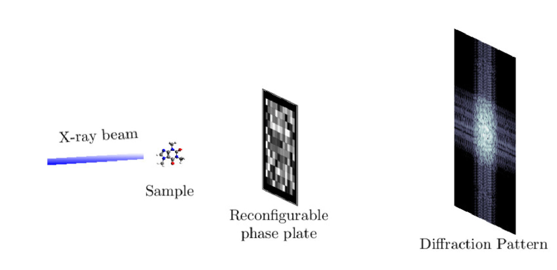 Figure 1
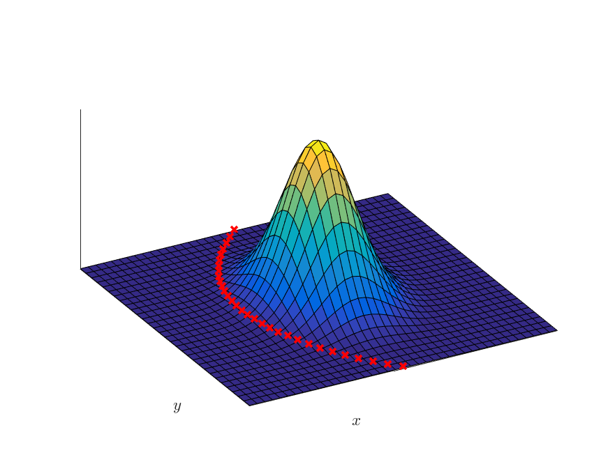 Figure 2
 Figure 3
 Figure 4
 Figure 5
 Figure 6
 Figure 7
 Figure 8
 Figure 9
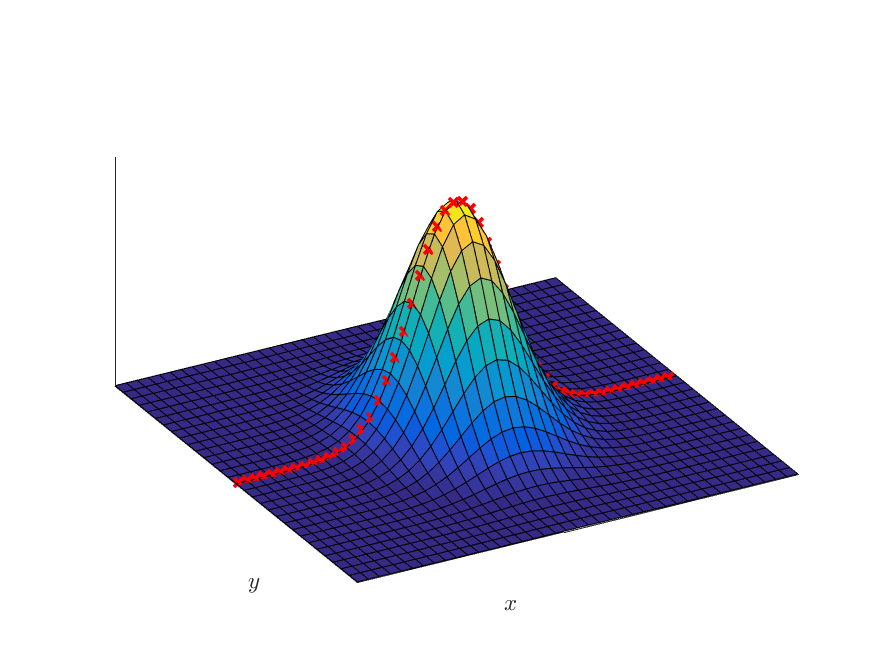 Figure 10
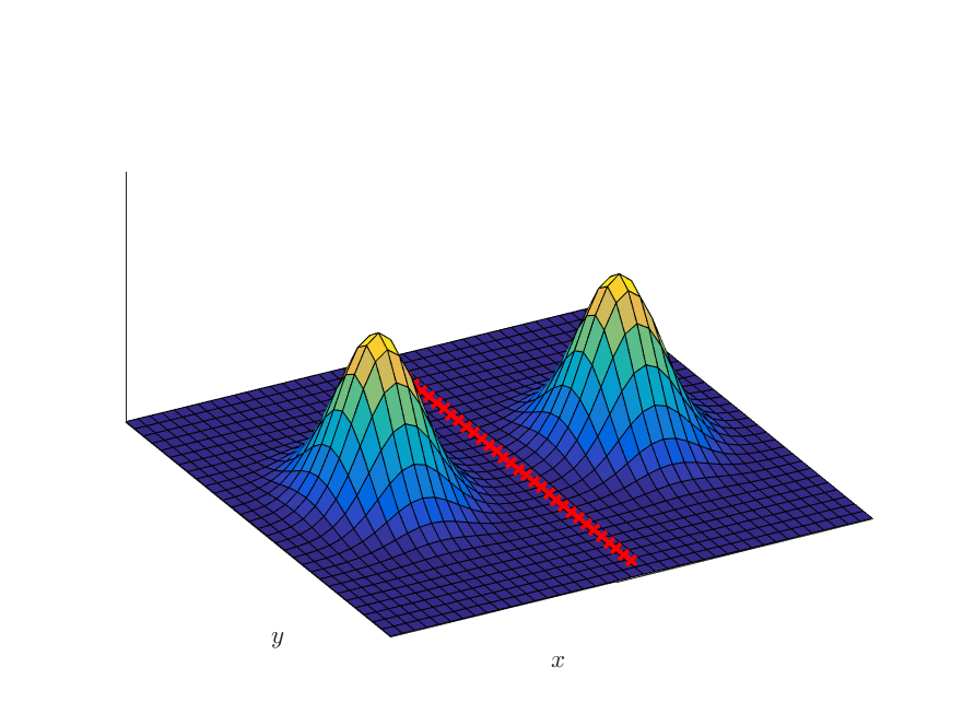 Figure 11
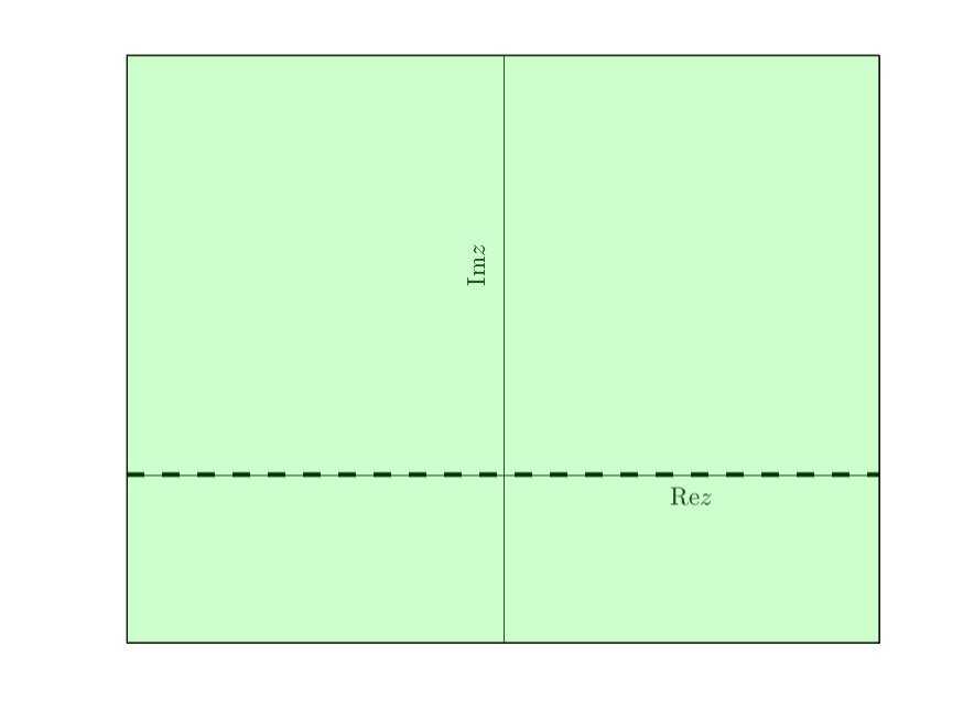 Figure 12
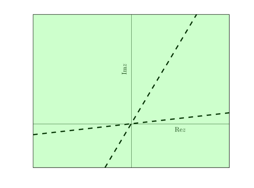 Figure 13
 Figure 14
Peer Reviews
No public reviews on file for this paper yet. If you reviewed it on a platform where reviews are public (OpenReview, ICLR, NeurIPS, ICML), you can paste yours below so the community can read it here.
Videos
No videos yet. Explain this paper in a talk, walkthrough, or lecture? Add one.
Phase Retrieval: Uniqueness and Stability
Philipp Grohs
Faculty of Mathematics
University of Vienna
Oskar-Morgenstern-Platz 1
A-1090 Vienna, Austria
,
Sarah Koppensteiner
Faculty of Mathematics
University of Vienna
Oskar-Morgenstern-Platz 1
A-1090 Vienna, Austria
and
Martin Rathmair
Faculty of Mathematics
University of Vienna
Oskar-Morgenstern-Platz 1
A-1090 Vienna, Austria
Abstract.
The problem of phase retrieval, i.e., the problem of recovering a function from the magnitudes of its Fourier transform, naturally arises in various fields of physics, such as astronomy, radar, speech recognition, quantum mechanics, and, perhaps most prominently, diffraction imaging. The mathematical study of phase retrieval problems possesses a long history with a number of beautiful and deep results drawing from different mathematical fields, such as harmonic analysis, complex analysis, and Riemannian geometry. The present paper aims to present a summary of some of these results with an emphasis on recent activities. In particular we aim to summarize our current understanding of uniqueness and stability properties of phase retrieval problems.
1. Introduction
The problem of phase retrieval, i.e., the problem of recovering a function from the magnitudes of its Fourier transform, naturally arises in various fields of physics, such as astronomy [40], radar [67], speech recognition [89], and quantum mechanics [85]. The most prominent example, however, is diffraction imaging, where in a basic experiment an object is placed in front of a laser which emits coherent electromagnetic radiation. The object interacts with the incident wave in a diffractive manner, creating a new wave front, which is described by Kirchhoff’s diffraction equation. An adequate approximation of the resulting wave front in the far field is given by the Fraunhofer diffraction equation, which essentially states that the wave front in a plane at a sufficiently large distance from the object is given by the Fourier transform (with appropriate spatial scaling) of the function representing the object; cf. [50] for an introduction to diffraction theory.
The aim in diffractive imaging is to determine the object from measurements of the diffracted wave. This objective is seriously impeded by the fact that measurement devices usually are only capable of capturing the intensities, and a loss of phase information takes place. Reconstructing the object from the far field diffraction intensities, the so-called diffraction pattern, therefore requires one to solve the Fourier phase retrieval problem
Given , find (up to trivial ambiguities).
The name “phase retrieval” accounts for the fact that recovery of the phase of is equivalent to recovering itself.
In microscopy a lens is employed to essentially invert the Fourier transformation and create the image of the object. While this is possible in the case of visible light, which has a wavelength of approximately , lenses which perform this task are not available for waves of much shorter wavelength (e.g. for x-rays with a wavelength in the range between and ). Since the spatial resolution of the optical system is proportional to the wavelength of light the direct approach using lenses can only achieve a certain level of resolution. In order to obtain high resolution it is necessary to compute the image from the diffraction pattern.
Determining objects from diffraction patterns—and therefore the question of phase retrieval—for the first time became relevant when Max von Laue discovered in 1912 that x-rays are diffracted when interacting with crystals, an insight for which he would be awarded the Nobel Prize in Physics two years later. The discovery of this phenomenon launched the field of x-ray crystallography. Crystallography seeks to determine the atomic and molecular structure of a crystal, i.e., a material whose atoms are arranged in a periodic fashion. In the diffraction pattern the periodicity of the crystalline sample manifests itself in the form of strong peaks (Bragg peaks) lying on the so-called reciprocal lattice; cf. [82]. From the position and the intensities of these peaks chrystallographers can deduce the electron density of the crystal. Over the course of the past century the methods of x-ray crystallography have developed into the most powerful tool for analyzing the atomic structure of various materials and have enabled scientists to achieve breakthrough results in different fields such as chemistry, medicine, biology, physics, and the material sciences. This is highlighted by the fact that more than a dozen Nobel Prizes have been awarded for work involving x-ray crystallography, the discovery of the double helix structure of DNA [101] being just one example. For an exhaustive introduction to x-ray crystallography the interested reader may have a look at [57, 76].
In 1980 it was proposed by David Sayre [92] to extend the approach of x-ray crystallography to noncrystalline specimens. Almost twenty years later, facilitated by the development of new powerful x-ray sources, Sayre et al.[80] for the first time successfully reconstructed the image of a sample with resolution at nanometer scale from its x-ray diffraction pattern. This approach is nowadays known as Coherent Diffraction Imaging (CDI). The process consists of two principal steps. First, the acquisition of one or multiple diffraction patterns, and second, processing the diffraction patterns in order to obtain the image of the sample, which is usually done by applying iterative phase retrieval algorithms. Plenty of CDI methods have been developed in recent years and have been employed to great success in physics, biology, and chemistry. See [81, 93] for very recent overviews of CDI methods, for their limitations and their achievements in various applications, and for algorithmic phase retrieval methods in diffraction imaging.
Even though the quest for recovering lost phase information has been omnipresent in physics for more than a century now, the phase retrieval problem has only very recently—with a few exceptions—started receiving great attention by the mathematics community. One notable exception is the work of Herbert Hauptman beginning in the 1950s. The direct methods developed by Hauptman [58], together with Jerome Karle have been applied with great success to determine the structure of many crystals. In 1985 Hauptman and Karle were awarded the Nobel Prize in Chemistry.
As a second significant exception we mention the work of Joseph Rosenblatt from the 1980s [91], where the problem of phase retrieval from Fourier magnitudes is studied in great generality.
Phase retrieval in the most general formulation is concerned with reconstructing a function in a space from the phaseless information of some transform of . The operator describing the transform, which will be denoted by , is mapping elements of into another space of either real- or complex-valued functions and is usually linear, i.e.,
[TABLE]
Furthermore, is usually nicely invertible, which means that has a bounded inverse.
In order to have a concrete example in mind one may think of and , the Fourier transform operator. In this case it is well known that is a unitary map.
Under the above assumptions the linear measurement process does not introduce a loss of information. However, the situation changes significantly if the phase information of the transform is absent. The problem arises of studying the obviously nonlinear mapping
[TABLE]
and its invertibility properties. Well-posedness in the sense of Hadamard of an inverse problem associated with requires
- (1)
existence of a solution, i.e., to be surjective; 2. (2)
uniqueness, i.e., to be injective; and 3. (3)
stability, meaning that the solution continuously depends on the data, i.e., to be continuous.
For the problem of phase retrieval, condition (1) amounts to identifying the image of the operator . The question is often of minor importance compared to (2) and (3) as it is simply assumed that the input data arise from the measurement process described by .
Provided that is a vector space—excluding trivial cases— is not injective due to the simple observation that
[TABLE]
Further ambiguities may occur, such as translations in the Fourier example but also less trivial ones. The first key question in the mathematical analysis of a phase retrieval problem is to identify all ambiguities. Depending on the context a particular source of ambiguities is either classified as trivial or as severe. If there exist severe ambiguities the phase retrieval problem is hopeless as there exist different objects yielding identical measurements. If on the other hand all occurring ambiguities are considered trivial, and may be identified () whenever . Let denote the quotient set. Then—by definition— is injective as mapping acting on and uniqueness in this new sense is ensured.
In order to study stability, has to be endowed with a reasonable topology first. In the case where is a normed space and the only ambiguities occurring are of the type shown in (1), usually the quotient metric
[TABLE]
is used. If there are other ambiguities, a suitable choice may be less obvious.
Beyond determining whether the mapping on is continuously invertible further continuity properties of the inverse are often studied such as (local) Lipschitz continuity.
If there are nontrivial ambiguities, i.e., if injectivity is not attained after identifying all trivial ambiguities or if the inverse is not continuous, one or both of the following measures may be taken in order to render the phase retrieval problem well-posed:
- (A)
Restriction of : The restriction , where is eventually injective (has a continuous inverse) if is chosen sufficiently small, consisting of a single element being the extremal, trivial example.
Restriction of to a smaller domain can be understood as imposing additional structural assumptions on the function to be reconstructed. In applications of the phase retrieval problem from Fourier measurements, for instance, it is typically sensible to demand that be nonnegative, as other functions do not hold a physical meaning. 2. (B)
Modification of : The idea is to suitably modify in order to soften the setback which is suffered by the subsequent removal of the phase information.
In the case of the Fourier phase retrieval problem this can be achieved by applying several different manipulations of before computation of the Fourier transform, e.g., using
[TABLE]
for known functions instead of . In the context of diffraction imaging this approach is common practice, as a physical system which produces measurements can often be implemented. In ptychography—a concept proposed by Walter Hoppe in the 1960s [61]—different sections of an object are illuminated one after another and the object is to be reconstructed from several diffraction patterns. For suitable, localized window functions , (2) serves as a reasonable mathematical model.
As a second example let us mention holography, invented by Dennis Gabor in 1947 [47]. In holography the diffracted waves interfere with the wave field of a known object. This idea amounts to an additive distortion of the wave field , where is a known reference wave.
To the best of our knowledge, these ideas (the restriction and modification approach that is) have been systematically implemented for the first time in a series of papers by Jaming [67, 68].
When studying a concrete phase retrieval problem with an application in the background it is useful to keep in mind that often there is a certain degree of freedom in the way the measurements are acquired. For instance, in diffraction imaging there is the fundamental observation that the wave in the object plane and the wave in the far field are connected in terms of the Fourier transform. However there are many different options in how to generate one or several diffraction patterns. Instead of viewing a phase retrieval problem as the analysis of a fixed operator one may as well include the question of how to design the measurement process in order to get a well-posed problem.
Beyond the question of well-posedness it is desirable to provide a method that recovers a function (at least the equivalence class ) from the observed measurements . Such a method could be an explicit expression of the inverse of . Mostly the aim of coming up with an explicit expression is rather hopeless. In practice iterative algorithms are employed, which serve as approximate inverses of the measurement mapping . A framework based on iterative projections which is often simple to implement and has proved to be very flexible was introduced by Gerchberg and Saxton [48] and was later extended by Fienup [44]. These methods have been employed to great empirical success, but due to the absence of convexity there is no guarantee of convergence. In recent years Candes, Strohmer, and Voroninski [32] have studied phase retrieval in a random setup and proposed an algorithm which provably recovers with high probability.
Phase retrieval problems have been studied in a rich variety of shapes. They can be distinguished between finite- and infinite-dimensional as well as between discrete and continuous phase retrieval problems. Furthermore phase retrieval problems differ in what kind of measurements are considered, i.e., the choice of the operator . The most common choice is that involves some sort of Fourier transform [2, 99, 60, 4, 78]. Moreover there is a huge body of research in the more abstract setting of frames, where it is assumed that is induced by a frame [14, 16, 28, 5]. Phase retrieval problems where the quantity of interest is assumed to arise as the solution of certain differential equations have also been studied [70, 69].
It is the aim of the present paper to present an overview of a selection of the aforementioned developments. In Section 2 we summarize our current understanding of abstract phase retrieval problems, that is, without precisely specifying the nature of the observed measurements.
Then we specialize to phase retrieval problems arising from (masked or windowed) Fourier transform measurements. The finite-dimensional case is considered in section 3, and the continuous infinite-dimensional setting in section 4. We present several (well-known and also new) results on uniqueness and stability of the corresponding phase retrieval problems.
Finally, we believe that phase retrieval offers researchers a unique combination of beautiful and deep mathematics as well as very concrete physical applications. It is our hope to convey some of our enthusiasm for this topic to the reader.
2. Abstract Phase Retrieval
From an abstract point of view, Fourier phase retrieval lends itself to the following interpretation: Of a function , we are given the absolute values of measurements given by bounded linear functionals. In the case of Fourier phase retrieval, the family of linear functionals are just the pointwise evaluation of the Fourier transform .
With this interpretation in mind, we can phrase the phase retrieval problem in a more abstract way. Throughout this section let denote a Banach space over and its topological dual space. Furthermore, let be a not necessarily countable index set. For a family of bounded linear functionals , we define the operator of phaseless measurements by
[TABLE]
where denotes the dual pairing. Due to the linearity, it is clear that for phase factors . We therefore introduce the equivalence relation and say does phase retrieval if the mapping
[TABLE]
is injective.
2.1. Injectivity
Suppose is a family of bounded linear functionals and . We then write . For a linear subspace of , let denote the annihilator of in .
Definition 2.1**.**
The family satisfies the complement property in if we have or for every .
Then the complement property is necessary for to be injective. In the real case, it is even sufficient.
Theorem 2.2**.**
Let be a Banach space over and a family of bounded linear functionals. Then the following hold:
- (i)
If is injective, then satisfies the complement property. 2. (ii)
If and satisfies the complement property, then is injective.
Theorem 2.2 has quite a history. It was first stated for finite dimensions in Balan, Casazza, and Edidin [14]. The arguments for the complex case should have been given more care. Bandeira et al. [16] spotted this oversight and gave an alternative proof for the complex case in finite dimensions. In doing so, they produced a series of characterizations for injectivity in finite dimensions. Moreover, they had the crucial insight for stability of phase retrieval by introducing a “numerical version” of the complement property (see section 2.2).
Ultimately, only a minor correction was necessary to repair Balan et al.’s proof and the same arguments also work in infinite dimensions. This is the proof we present below, which can also be found in [5, 24, 28].
Proof.
(i) Let be injective for and arbitrary. Assume that there is a nonzero and let . We have to show that . First note that
[TABLE]
Hence . As is assumed to be injective, there exists a phase factor such that . Since we have and then
[TABLE]
which implies that . Now the injectivity of implies as expected.
(ii) Suppose is not injective, this means that there exist such that . Since consists of real-valued linear functionals, the signed measurements of and with respect to can only differ by a factor of . We therefore consider the following partition of the index set : Let ; then .
Consequently, and . But by assumption at least one of those annihilators consists only of [math]. Hence or and therefore is injective. ∎
For the Paley–Wiener space () of real-valued band-limited functions, one can show that the complement property holds for families of point-evaluations if the sampling rate exceeds twice the critical density [5]. Since is a real-valued Banach space, this implies that phase retrieval is possible.
For complex Banach spaces, the complement property is not sufficient. Hence other methods need to be employed to study injectivity. For Fourier-type measurements, these tools often come from complex analysis (see sections 3 and 4).
We now turn to the finite-dimensional case. The complement property implies that needs to span the whole space and must be overcomplete for phase retrieval to be possible. In other words, must be a frame.
In the remainder of this section, we state necessary and sufficient conditions on the number of frame elements of to do phase retrieval. The first result is an easy consequence of the complement property.
Corollary 2.3**.**
If , then cannot be injective for any family with elements.
Proof.
We partition into two sets with at most elements. This yields and , clearly violating the complement property. ∎
For , the converse statement also holds for “almost all” frames. To make this more precise, we need some terminology of algebraic geometry.
An algebraic variety in is the common zero set of finitely many polynomials in . By defining algebraic varieties in as closed, we obtain the Zariski topology. Note that this topology is coarser than the Euclidean topology on , meaning that every Zariski-open set is also open with respect to the Euclidean topology. Furthermore, nonempty Zariski-open sets are dense with respect to the Euclidean topology and have full Lebesgue measure in [16, 34].
We say a generic point in satisfies a certain property, if there exists a nonempty Zariski-open set with this property. By the above, this means that if a certain property holds for a generic point, it holds for almost all points in .
Now we identify a frame of elements with a matrix of full rank. Hence the set of frames with elements in , i.e., the set of matrices of full rank in , is a nonempty Zariski-open set and it makes sense to study generic points within the set of frames. We call those generic points generic frames.
The following theorem is due to Balan, Casazza, and Edidin [14]. Together with Corollary 2.3, it (almost) characterizes the injectivity of phase retrieval in .
Theorem 2.4**.**
If , then is injective for a generic frame with elements.
For phase retrieval in , Bandeira et al. [16] conjectured an analogous characterization with being the critical number of frame elements. They also gave a proof in dimensions . Conca et al. [34] (see also [73]) proved the following theorem, confirming the sufficient part of the -Conjecture.
Theorem 2.5**.**
Let . If , then is injective for a generic frame with elements.
Conversely, a frame in with elements does not allow phase retrieval in dimensions [34]. But the -Conjecture does not hold in general: Vinzant [97] gave an example of a frame with elements in which does phase retrieval. For necessary lower bounds in general dimension, we refer the interested reader to Wang and Xu [100]. A more in-depth account of the history of necessary and sufficient bounds for phase retrieval in can be found in [24]. Furthermore, Bodmann and Hammen [20, 21] developed concrete algorithms and error bounds for phase retrieval with low-redundancy frames.
2.2. Stability
Once the question of injectivity is answered positively, the question of stability arises. Stability refers to the continuity of the operator . To this end, we need to introduce a topology on and find a suitable Banach space with . The natural choice for is the quotient metric
[TABLE]
The analysis space for frames in separable Hilbert spaces is the sequence space . We will consider the stability of phase retrieval for continuous Banach frames in this section. There, the appropriate generalization of is an “admissible” Banach space such that the range of the coefficient operator
[TABLE]
is contained in .
Definition 2.6**.**
Let be a -compact topological space. A Banach space is called admissible if it satisfies the following properties:
- (i)
The indicator function of every compact set satisfies . 2. (ii)
The Banach space is solid; this means that whenever for all . 3. (iii)
The elements of with compact support are dense in .
These properties are quite reasonable. Indeed, all -spaces for are admissible Banach spaces and violates only the last point unless is already compact.
Now we are in a position to define stability of phase retrieval precisely.
Definition 2.7**.**
Let be a family of bounded linear functionals and and admissible Banach space such that . We say that the phase retrieval of is stable (with respect to ) if there exist constants such that
[TABLE]
Moreover, let denote the optimal lower and upper Lipschitz bound respectively.
Definition 2.8**.**
Suppose that is a family of bounded linear functionals such that is continuous. We call a continuous Banach frame if there exists an admissible Banach space such that the following is satisfied:
- (i)
There exist positive constants such that
[TABLE]
Moreover, let denote the optimal constants satisfying (4). 2. (ii)
There exists a continuous operator , the so-called reconstruction operator, satisfying
[TABLE]
The requirement for to be a frame is a natural one. In fact, if maps into an admissible Banach space, the solidity implies . Hence, stability in the sense of (3) implies the frame inequality (4) by taking . For the upper inequalities, we even have equivalence.
Proposition 2.9**.**
If is a family of continuous linear functionals such that maps into an admissible Banach space, then .
Again the solidity of the admissible Banach space plays an integral role in the proof. As the rest follows from straightforward estimates, we omit the proof and refer the interested reader to [5, 28].
The remainder of the section deals with the lower inequality in (3). We start by mentioning an interesting result about the continuity of the inverse operator , which can be regarded as a weaker form of stability.
Theorem 2.10**.**
Let be a continuous Banach frame and injective. Then is continuous on the range of .
Proof idea.
We need to show that the convergence of the image sequence in implies the convergence of in . The idea is to link the convergence of to the convergence of the signed measurements . This is the technical and lengthy part of the proof, and we refer the interested reader to [5] for the details. Once this relation is established, one can use the continuous reconstruction operator to obtain . ∎
As an easy consequence of Theorem 2.10, we obtain stability of phase retrieval in finite-dimensional Banach spaces.
Theorem 2.11**.**
Let be a finite-dimensional Banach space. If is a frame that does phase retrieval, then has a lower Lipschitz bound .
Proof.
Note that the existence of a positive lower Lipschitz bound in (3) is equivalent to being Lipschitz continuous with constant .
By Theorem 2.10, the inverse is continuous on . Since is finite-dimensional, the closed unit ball is compact, and therefore is uniformly continuous on . By using the scaling invariance of and playing everything back into the unit ball , the Lipschitz continuity follows in a series of straightforward estimates. ∎
The result of Theorem 2.11 was proved first for the real case in [15, 16]. Cahill, Casazza, and Daubechies [28] gave a proof for the complex case. The proof above is from [5].
For their proof of stability in finite dimensions, Bandeira et al. [16] introduced the following “numerical” version of the complement property, which relates to stability as the complement property relates to injectivity.
Definition 2.12**.**
The family satisfies the -strong complement property in if there exists a such that
[TABLE]
Moreover, let denote the supremum over all satisfying (5).
Theorem 2.13**.**
Let be a Banach space over and a continuous Banach frame. Then there exists a constant such that
[TABLE]
In the real case, the constant is . For the complex case, the constant can be chosen .
Remark 2.14**.**
For the real case, one can also show that for some . This implies that the -strong complement property is not only necessary, but also sufficient for stability in real Banach spaces. In this sense, it mirrors the behavior of the complement property.
Unfortunately, the sufficiency cannot be exploited for (global) stability: On one hand, phase retrieval is always stable in finite dimensions by Theorem 2.11 and on the other hand, we will see that the -strong complement property can never hold in infinite dimensions.
Proof.
Let . Then there exist a subset and with such that
[TABLE]
Now set and . Due to the solidity of , we obtain
[TABLE]
where we used the reverse triangle inequality in the second line.
By definition of , we conclude
[TABLE]
In the real case, we are done since
[TABLE]
The complex case proves to be more difficult. A series of elementary estimates are necessary to bound away from zero. We refer the interested reader to the original article [5]. ∎
Remark 2.15**.**
The computations in the proof of Theorem 2.13 also yield an estimate on local stability constants. More precisely, suppose a fixed can be decomposed according to such that , and that (6) holds for . Then there exists such that
[TABLE]
Thus, and yield similar measurements even though they are very different from each other.
Theorem 2.13 implies that the -strong complement property is necessary for stability. Bandeira et al. [16] gave a proof of this for the real case and conjectured the complex case, which was proved in [5].
For finite dimensions, phase retrieval is always stable by Theorem 2.11. In particular, the -strong complement property is satisfied. In infinite dimensions, we will see that continuous Banach frames cannot satisfy the -strong complement property, hence phase retrieval is always unstable in this case. To show this, we follow [5] and prove an intermediate result, which is interesting in its own right. It states that there cannot exist continuous Banach frames in infinite dimensions with compact index set .
Proposition 2.16**.**
Suppose is an infinite-dimensional Banach space and a compact index set. Then any family with continuous mapping fails to satisfy the lower frame inequality. This means that for every there exists an such that
[TABLE]
Proof.
Let . By continuity of the mapping , there exists for every an open neighborhood such that
[TABLE]
Since is compact, the open covering admits a finite subcover . Now set and for to obtain a partition of which satisfies the following for all :
[TABLE]
Clearly, we have
[TABLE]
for all . After multiplication with the characteristic function and summing over , we obtain
[TABLE]
Now the solidity of implies
[TABLE]
for all . Since is infinite-dimensional, there exists a nonzero such that for all . Consequently, the sum on the right-hand side vanishes for and we obtain the claim. ∎
Theorem 2.17**.**
Let be an infinite-dimensional Banach space over and a continuous Banach frame. Then does not satisfy the -strong complement property.
Proof.
We need to show that the -strong complement property is not satisfied. This means that for every we can find a subset and such that
[TABLE]
We start with an arbitrary with . Since is an admissible Banach space where compact elements are dense, there exists a nested sequence of compact subsets with such that
[TABLE]
Hence, there exists a such that
[TABLE]
Setting , we obtain .
On the other hand, we can use Theorem 2.16 for the compact set to find an such that
[TABLE]
∎
Corollary 2.18**.**
Let be an infinite-dimensional Banach space over and a continuous Banach frame. Then cannot do stable phase retrieval. This means that for every , there exist with but .
Proof.
This is an immediate consequence of the fact that the -strong complement property is necessary for stability by Theorem 2.13, but continuous Banach frames in infinite dimensions cannot satisfy it by Theorem 2.17. ∎
Remark 2.19**.**
Phase retrieval in infinite dimensions cannot be stable for continuous Banach frames by Corollary 2.18. On the other hand, Theorem 2.11 states that it is always stable in finite dimensions. The natural question that arises is the following: Suppose is a sequence of finite-dimensional subspaces and let denote the stability constant for the subspace in (3). How fast does the stability constant degenerate as the dimension increases?
It turns out, this can be rather rapidly: Cahill, Casazza, and Daubechies [28] considered subspaces of increasing dimension in the Paley–Wiener space and showed that the stability constant degrades exponentially fast in the dimension. Even worse degeneration can be observed for the short-time Fourier transform with Gaussian window on : Alaifari and one of the authors [6] constructed a sequence of subspaces whose stability constant degrades quadratically exponentially in the dimension.
3. Finite Dimensional Phase Retrieval
This section is devoted to phase retrieval from Fourier measurements in the finite-dimensional setting. The first emphasis lies on identifying ambiguities for phase retrieval from phaseless discrete time Fourier transform (DTFT) measurements. The second main focus lies on discussing various strategies to remove ambiguities, and yield well-posed reconstruction problems. These strategies include priors such as assuming sparsity of the signals to be reconstructed or tweaking of the measurement process, for example by increasing the number of measurements and/or by introducing randomness.
3.1. The classical Fourier Phase Retrieval Problem
In the following we will discuss the problem of recovering a signal from its phaseless Fourier transform. We consider multidimensional discrete signals. This means that for , a discrete signal is a complex-valued function on
[TABLE]
Definition 3.1**.**
The discrete-time Fourier transform of a discrete signal is defined by
[TABLE]
where the normalization is understood componentwise and denotes the inner product on .
The problem of Fourier phase retrieval can now be stated as follows.
Problem 1** (Fourier phase retrieval, discrete).**
Recover from .
Remark 3.2**.**
For the squared modulus of its DTFT is a trigonometric polynomial and is uniquely defined by its values on a suitable, finite sampling set . The problem of recovering from the full Fourier magnitude is therefore equivalent to the problem of recovering from finitely many samples of the Fourier magnitude .
The goal is to characterize all ambiguous solutions of Problem 1 for a given signal . Before we do so let us draw the attention of the reader to Fienup’s paper [45] from the 1970s where the following observation is made:
Experimental results suggest that the uniqueness problem is severe for one-dimensional objects but may not be severe for complicated two-dimensional objects.
Within this section we will give a rigorous explanation of this phenomenon.
Before we identify ambiguities, we have to explain what it means to reflect and translate a signal . We define the reflection operator on by
[TABLE]
and the translation operator for by
[TABLE]
where the modulo operation is to be understood componentwise. Similarly the conjugation operation will be understood componentwise. For and we will write and for short.
Proposition 3.3**.**
Let . Then each of the following choices of yields the same Fourier magnitudes as , i.e., :
- (i)
* for ;* 2. (ii)
* for ;* 3. (iii)
.
Proof.
The statement follows from (i) linearity of the Fourier transform, (ii) translation amounts to modulation in the Fourier domain and (iii) reflection and conjugation amounts to conjugation in the Fourier domain. ∎
The ambiguities described in Proposition 3.3, as well as combinations thereof, are considered trivial. By identifying trivial ambiguities an equivalence relation is introduced on , i.e.,
[TABLE]
To determine all ambiguities we will study the so-called -transform.
Definition 3.4**.**
For the -transform is defined by
[TABLE]
The question of uniqueness of Problem 1 is closely connected to whether the -transform has a nontrivial factorization, as we shall see.
Definition 3.5**.**
A polynomial of one or several variables is called reducible if there exist nonconstant polynomials and such that . Otherwise is called irreducible.
In what follows, let denote a multivariate polynomial. Its degree is defined with respect to each coordinate, i.e.,
[TABLE]
Later we will need to consider the mapping . Clearly, its singularities can be removed by multiplication with a suitable monomial. Indeed,
[TABLE]
is again a polynomial. Finally, let denote the largest exponent (component-wise) such that is a divisor of . Thus there exists a unique polynomial such that
[TABLE]
To shed some more light onto these concepts we consider a concrete example.
Example 3.6**.**
Let us consider the polynomial on defined by
[TABLE]
We see that and that . Moreover,
[TABLE]
and
[TABLE]
It is not difficult to verify that for any polynomial it holds that
[TABLE]
and that
[TABLE]
The following theorem characterizes all ambiguities of the discrete Fourier phase retrieval problem.
Note that multiplication of the Z-transform of by a unimodular factor by linearity corresponds to multiplication of the itself. Multiplication of for corresponds to translation in the signal domain, and flipping the -transform, i.e., passing over to , amounts to reflection and conjugation in the signal domain.
Theorem 3.7**.**
Let and let denote their respective -transforms. Then if and only if there exist a factorization , a constant with , and such that
[TABLE]
Proof.
First we show the necessity of the statement. Suppose is an ambiguous solution with respect to . By definition and thus, using the notation
[TABLE]
we observe that . For the squared magnitude of the Fourier transform it therefore holds that
[TABLE]
where conjugation and the reciprocal are to be understood component-wise. By the assumption that and by analytic continuation, we obtain
[TABLE]
Now factorize and into irreducible polynomials:
[TABLE]
After multiplying both sides of (8) by , we obtain the equality
[TABLE]
Since is irreducible it follows that is irreducible. Moreover we have that . Obviously the same arguments can be applied to .
By uniqueness of the factorization it follows that
[TABLE]
and that . Now let be a maximal subset of such that divides and let . Without loss of generality (w.l.o.g.) we assume that with and that divides (this can be achieved by permutation of the index sets). Due to irreducibility it must hold that
[TABLE]
for suitable nonzero constant , and, consequently that
[TABLE]
where is another nonzero constant. Use (10) and (11) and cancel (9) by the respective factors to obtain that
[TABLE]
for a constant . From the maximality of it follows that divides , and thus that divides . Therefore there exists such that
[TABLE]
Hence we get that
[TABLE]
Note that , since
[TABLE]
Consequently, we obtain for suitable and the factorization
[TABLE]
with and .
For the sufficiency let be a polynomial of the form (7). Then
[TABLE]
∎
For to have nontrivial ambiguities it is therefore necessary that its -transform be reducible. Note that this is not sufficient in general, as the factors of may possess symmetry properties such that a flipping does not introduce nontrivial ambiguities. Nevertheless, this observation yields an upper bound on the number of ambiguous solutions for denoted by
[TABLE]
Corollary 3.8**.**
Let and let denote its -transform. Then , where denotes the number of nontrivial factors of .
In the one-dimensional case the -transform is a polynomial of one variable of order . By the fundamental theorem of algebra, has roots and can be expressed as a product of linear factors. Assuming none of the roots lie on the unit circle and coincides each element in the power set of the set of roots (except for the empty set and the full set) induces a nontrivial ambiguity. The situation in the higher dimensional case is radically different, as shown by Hayes and McClellan [59].
Theorem 3.9** ([59]).**
Let denote the set of complex polynomials of variables with order and let denote the degrees of freedom of . We identify with . Then the set of reducible polynomials in is a set of measure zero (as a subset of ).
Corollary 3.8 together with Theorem 3.9 yields the following result.
Corollary 3.10**.**
If , then for any fixed the set is of measure zero.
If , then for any fixed the set is of measure zero.
A frequently used prior restriction on the signals is to require sparsity. To assume sparsity of the underlying signal appears natural in many practical applications such as crystallography or astronomy. For a thorough discussion of sparse phase retrieval among other topics, we refer the reader to the excellent survey articles [19, 65]. We choose to present at this point one particular result on sparse Fourier phase retrieval which nicely complements the univariate statement in Corollary 3.10.
Theorem 3.11** ([66]).**
For let denote the set of -sparse signals in , i.e., the set of vectors that possess at most nonzero entries, with aperiodic support. Then almost all are uniquely determined by up to a constant sign factor within .
3.2. Fourier phase retrieval using masks
In the one-dimensional case the modulus of the DTFT is not a useful representation for most signals. A popular strategy in order to increase information and introduce redundancy to counter the loss of phase is to allow for masked Fourier measurements. By a mask we mean a function with the corresponding phaseless measurement process being described by
[TABLE]
where denotes the pointwise product in . In order to attain a sufficient amount of information it is common to employ not one but several different masks. We essentially distinguish between two types of this kind of measurement. First, in case of the short-time Fourier (STFT) measurements, the various masks are generated by applying shifts to a fixed window function. This is the mathematical model behind ptychography, where an aperture is slid over the sample to illuminate different parts (see Figure 1). Second, the various masks can be chosen in a completely unstructured manner.
We shall see that the uniqueness issues which have been discussed in the first part of this section can be removed if the masks are suitably chosen. In the multivariate setting a generic signal is uniquely (up to trivial ambiguities) determined by the modulus of its DTFT; cf. Corollary 3.10. However, there are deterministic signals—namely, those which possess a reducible Z-transform—for which uniqueness fails to hold. In a randomized setting where one can observe the modulus of the DTFT of and the entries of the mask are drawn randomly according to a suitable distribution, uniqueness holds with probability one provided that the support of the signal satisfies a rather weak assumption, as shown by Fannjiang [43].
3.2.1. Discrete Short-Time Fourier Phase Retrieval
In this section, we consider finite signals in the complex Hilbert space with inner product
[TABLE]
The discrete Fourier transform maps finite signals to finite signals and is defined as
[TABLE]
Its inverse is given by
[TABLE]
and with the normalization above, Plancherel’s theorem is of the form
[TABLE]
We define the (circular) translation and modulation operators by
[TABLE]
for . In the following, we identify the finite signal with its periodic extension and just write for the circular translated signal.
Since a modulation in time corresponds to a shift in frequency, operators of the form are called time-frequency shifts for . Note that time-frequency shifts do not commute, but satisfy the following commutation relation.
Lemma 3.12**.**
Let . Then
[TABLE]
where denotes the standard symplectic matrix.
We omit the proof, as it is a straightforward verification.
The discrete short-time Fourier transform of with respect to the window is defined by
[TABLE]
for .
For fixed window , the short-time Fourier transform is a linear operator that maps finite signals in to finite signals in . Due to the linearity, we again have the trivial ambiguity for phase factors . Now the question is whether these are the only ambiguities, and how can the original signal be recovered.
Problem 2** (discrete short-time Fourier phase retrieval).**
Suppose . Recover from up to a global phase factor when is known.
Whether Problem 2 has a solution depends on the choice of the window . A sufficient condition is that the short-time Fourier transform does not vanish anywhere on . In the following we aim at proving this fact.
The main insight for short-time Fourier transform phase retrieval comes from the following formula which also appears in [49] and will be proved in what follows.
Proposition 3.13**.**
Let . Then
[TABLE]
where denotes the standard symplectic matrix.
The proof of formula (13) is elementary and requires only two things: the covariance property, which is an easy consequence of the commutation relations (12), and a version of Plancherel’s theorem for the short-time Fourier transform.
Lemma 3.14** (Covariance Property).**
Let . Then
[TABLE]
Proof.
Note that time-frequency shifts are unitary operators on . Hence
[TABLE]
where we used the commutation relation (12) on the second line. ∎
Proposition 3.15** (Orthogonality Relations).**
Let . Then
[TABLE]
Proof.
We write the short-time Fourier transform as and use Plancherel’s theorem in the sum over :
[TABLE]
∎
Proof of Proposition 3.13.
First note that , where denotes the identity matrix. Consequently,
[TABLE]
by Lemma 3.14. Hence, we obtain
[TABLE]
where we used the orthogonality relations (14) in the last step.
Note that for a suitable phase factor . But these phase factors cancel when we bring both time-frequency shifts to the other side, hence
[TABLE]
∎
We can now prove a sufficient condition on the window to allow phase retrieval.
Theorem 3.16**.**
*Let be a window with for all . Then any can be recovered from up to a global phase factor. *
Proof.
By Proposition 3.13 we have
[TABLE]
If has no zeros, we can recover . Now we apply the inverse discrete Fourier transform to and obtain
[TABLE]
Setting yields
[TABLE]
and we recover the signal up to a global phase factor after dividing by . ∎
Theorem 3.16 also appears in [22], where it is proved with the methods introduced in [16]. Moreover, the authors also give examples and counterexamples of window functions satisfying for all .
Different variants of Problem 2 have been studied over the years. One possible, alternative point of view is to restrict the problem to either sparse signals or signals that do not vanish at all in favor of weaker assumptions imposed on the window. We showcase one illustrative result in this direction and point the reader toward the articles by Jaganathan, Eldar, and Hassibi [64] and Bendory, Beinert, and Eldar [19] which give an excellent overview on both uniqueness and algorithmic aspects of short-time Fourier transform phase retrieval.
Theorem 3.17** ([42]).**
Let be a window of length , where the length of is defined as the length of the smallest interval in containing the support of . Then every with nonvanishing entries is defined uniquely by provided
- (i)
the discrete Fourier transform of defined as is nonvanishing; 2. (ii)
; and 3. (iii)
* and are coprime.*
Next, we study the case of a randomly picked window.
Theorem 3.18**.**
There exists a set of measure zero such that for all the family allows for phase retrieval, i.e., the mapping
[TABLE]
is injective.
Proof.
To prove the theorem we closely follow the proof techniques used by Bojarovska and Flinth [22, Proposition 2.1] where a similar statement is shown.
By Theorem 3.16 and since there are only finitely many , it suffices to show that there exists a set of measure zero such that for arbitrary but fixed it holds that
[TABLE]
Since is unitary there exists an orthonormal basis of and such that
[TABLE]
where denotes the conjugate transpose of the row vector . If we expand the window with respect to the basis, i.e., , we get that
[TABLE]
Since is a manifold of codimension one in and is an isometry it follows that
[TABLE]
is of measure zero, and indeed for all it holds that . ∎
3.2.2. Phase retrieval with equiangular frames
This subsection is devoted to presenting the work by Balan et al. [13], “Painless reconstruction from magnitudes of frame coefficients.” The main results reveal that the structure of certain, carefully designed frames can be leveraged to derive explicit reconstruction formulas for the corresponding phase retrieval problem.
To specify the properties of the frames that we shall consider we give a few definitions.
Definition 3.19**.**
Let be a -dimensional Hilbert space. A finite family of vectors is called
- •
-tight frame, with frame constant if all can be reconstructed from the sequence of frame coefficients according to
[TABLE]
- •
uniform A-tight frame if it is an -tight frame and there is such that for all .
- •
-uniform A-tight (or equiangular) frame if it is a uniform -tight frame and there exists such that for all .
A simple example of an equiangular frame is given by the so-called Mercedes-Benz frame.
Example 3.20**.**
Let . Then the three vectors defined by
[TABLE]
form a -uniform -tight frame.
The size of a -uniform tight frame is bounded from above in terms of the dimension of the space.
Theorem 3.21** ([13, Proposition 2.3]).**
Let denote the number of vectors in a -uniform tight frame on a -dimensional real or complex Hilbert space . Then in the real case, and in the complex case, respectively.
We shall call a -uniform tight frame maximal if it is of maximal size, i.e., if in the real case, and in the complex case.
Definition 3.22**.**
Let be a real or complex Hilbert space. A family of vectors with and is said to form mutually unbiased bases if for all and it holds that
[TABLE]
If form mutually unbiased bases, then it follows from the defining equality (15), that for fixed we have that is an orthonormal basis. Moreover, the magnitudes of the inner products attain just the three values , and . In that sense the notion of mutually unbiased bases may be regarded as a relaxation of equiangular frames, which allows for only two values.
As in the case of equiangular frames the size of mutually unbiased bases is bounded from above in terms of the dimension.
Proposition 3.23** ([13, Proposition 2.6]).**
There are at most mutually unbiased bases in a -dimensional complex Hilbert space .
To every we associate the operator
[TABLE]
which is (up to a scaling factor) the projection onto the span of . In particular, is uniquely determined up to a sign factor by .
A special case of the reconstruction formula reads as follows.
Theorem 3.24** ([13, Theorem 3.4], special case).**
Let be a -dimensional complex Hilbert space and suppose that satisfies one of the following assumptions:
- (i)
* forms a maximal -uniform -tight frame.* 2. (ii)
* forms mutually unbiased bases.*
Given a vector with associated self-adjoint rank-one operator , then
[TABLE]
where denotes the identity operator on .
Remark 3.25**.**
Note that in [13] the preceding theorem is phrased in terms of -uniform tight frames that give rise to so-called projective -designs. The assumptions made in the version as stated above are stronger; see [13, Example 3.3].
Furthermore, note that since the frame is assumed to be -tight, it follows that
[TABLE]
thus, the right-hand side of (16) can be computed from the magnitudes of the inner products .
We conclude this subsection with a concrete example of mutually unbiased bases that have Gabor structure. The construction we consider goes back to Alltop [8]; see also [94].
Lemma 3.26** (Alltop).**
Let be prime, let denote the -th unit root, and define
[TABLE]
Then it holds that
[TABLE]
With the help of Lemma 3.26 we establish the following.
Theorem 3.27**.**
Let be prime, let denote the -th unit root, and define . For define vectors
[TABLE]
and let denote the canonical basis of .
Then form mutually unbiased bases, and in particular for all it holds that
[TABLE]
Proof.
We only need to check that (15) holds true. Then the reconstruction formula follows by applying Theorem 3.24. The case follows from the preceding lemma and from the definition of , respectively. Thus, it remains to show that for the magnitude of the inner product equals . We distinguish the two cases (a) and (b) .
Since , where is defined as in (17) we have in case (a) that
[TABLE]
where the last equality follows again from Lemma 3.26. In case (b) we have that
[TABLE]
∎
3.2.3. Lifting Methods
Inspired by the pioneering work of Candès et al.[29, 32] which produced the now famous PhaseLift algorithm, the use of methods from semidefinite programming to solve phase retrieval problems has become hugely popular in recent years.
Given let us consider the associated phase retrieval problem, i.e., the problem of finding from observations
[TABLE]
PhaseLift and related methods are based on the idea of lifting the signal of interest to a rank (at most) one matrix by virtue of
[TABLE]
where denotes the conjugate transpose of . Note that determines up to a constant phase factor.
Since
[TABLE]
the original phase retrieval can be reformulated in terms of an optimization problem in :
[TABLE]
In order to obtain a feasible problem—rank minimization is NP-hard in general—(19) is relaxed by means of trace minimization, which gives rise to the semidefinite program
[TABLE]
As it turns out (20) and the original phase retrieval problem are equivalent if the measurement vectors are sufficiently many and picked at random.
Theorem 3.28** ([32]).**
Consider arbitrary. Suppose that
- •
the number of measurements obeys , where is a sufficiently large constant and
- •
the measurement vectors are independently and uniformly sampled on the unit sphere of .
Then with probability at least , where is a positive constant, (20) has as its unique solution.
Let us point out that [32] also contains a result that guarantees robust reconstruction of by an adequate modification of (20) from noisy measurements
[TABLE]
where models the effect of noise. Since our main focus lies on Fourier-type measurements we refrain from going into detail.
In a followup article it was shown by Candès, Li, and Soltanolkotabi [30] that also Fourier-type measurements can be accommodated for in the PhaseLift framework if random masks are employed. In the case of masked Fourier measurements, with masks , the quantities that can be observed are
[TABLE]
where and To set up the corresponding semidefinite program it is enough to use
[TABLE]
as replacements for in (20):
[TABLE]
Again, if the measurements are sufficiently many and suitably randomized the trace relaxation (21) is exact.
Theorem 3.29** ([30]).**
Let be arbitrary. Suppose that
- •
the number of coded diffraction patterns obeys for some numerical constant ; and
- •
the diagonal matrices , are independent and identically distributed (i.i.d.) copies of a diagonal matrix , whose entries are themselves i.i.d. copies of a random variable , where is assumed to be symmetric, as well as
[TABLE]
Then with probability at least it holds that is the only feasible point of (21).
In particular, Theorem 3.29 implies uniqueness with high probability when using on the order of random masks, which amounts to a total number of measurements. In the same setting, Gross, Krahmer, and Kueng [56] were able to prove that in fact masks are sufficient.
A major drawback of PhaseLift and related methods is that with increasing dimension the algorithms become computationally demanding. After all, the lifting shifts the problem from an -dimensional space to an -dimensional space. A more efficient procedure that does not rely on lifting the signal and still comes with recovery guarantees is the Wirtinger flow as proposed by Candès, Li, and Soltanolkotabi [31]. Wirtinger flow is based on carefully picking an initialization using a spectral method followed by an iterative scheme akin gradient descent.
3.2.4. Polarization Methods
Within this subsection we outline the approach taken by Alexeev et al. [7] and summarize some results based upon these ideas.
Again, the objective is to reconstruct up to a phase factor from measurements , as given by (18). At the heart of the proposed reconstruction method lies the elementary Mercedes-Benz polarization identity,
[TABLE]
where . Apply (22) to and to obtain
[TABLE]
thus, in particular the relative phase
[TABLE]
between two measurements can be observed under the assumption that we have access to supplementary phaseless measurements , and provided that and do not vanish. Hence in that case phase information can be propagated, meaning that assuming that, the phase of is known, one can also reconstruct the phase and thus the value of .
It turns out to be very useful to represent the measurement setup as a graph with each vertex corresponding to one of the measurement vectors and vice versa. To the edge between vertices and the three new measurement vectors
[TABLE]
are attached. Note that if is fully connected we end up with measurement vectors. The main result in [7] guarantees that if the vectors are drawn randomly and is of order , then the graph can be adaptively pruned in such a way that the resulting graph possesses at most edges, and, moreover, that can be uniquely recovered from the corresponding measurements. The statement holds true with high probability.
It is important to mention that the proposed algorithm does in general not produce an ensemble of measurement vectors such that any can be recovered since the process of selecting the measurement vectors depends on the observed intensities . Furthermore, the algorithm can be adapted in such a way that also reconstruction from noisy measurements can be accommodated.
In a followup paper [17] it was shown by some of the authors of [7] and collaborators that a similar approach can be taken when dealing with masked Fourier measurements. To be more concrete, the main results reveal that the proposed randomized procedure yields masks such that any signal is uniquely determined up to global phase by the corresponding phaseless masked Fourier measurements.
A robust version of the algorithm, which is capable of handling noisy masked Fourier measurements, was recently introduced by Pfander and Salanevich [87].
4. Infinite Dimensional Fourier Phase Retrieval
This section is devoted to phase retrieval problems where the underlying operator is the continuous Fourier transform or variants thereof. Such problems are typically studied within the scope of complex analysis. As is widely known analytic functions of several complex variables behave very differently from univariate holomorphic functions. As we shall see a qualitative gap between the one-dimensional and the multidimensional cases is also encountered for the problem of Fourier phase retrieval.
4.1. The Classical Fourier Phase Retrieval
For signals of continuous variables we will use the following normalization of the Fourier transform.
Definition 4.1**.**
Let . The Fourier transform of is defined by
[TABLE]
For , the Fourier transform is to be understood as the usual extension.
The problem of continuous Fourier phase retrieval can now be stated as follows.
Problem 3** (Fourier phase retrieval, continuous).**
Suppose and is compactly supported. Recover from .
We start with identifying the trivial ambiguities. As in the discrete case, let denote the translation operator for and the reflection operator .
Proposition 4.2**.**
Let . Then each of the following choices of yields the same Fourier magnitudes as , i.e., :
- (i)
* for ;* 2. (ii)
* for ;* 3. (iii)
.
The proof is straightforward. Again the ambiguities of Proposition 4.2 and their combinations are considered trivial ambiguities.
A standard assumption is to consider only compactly supported functions. In the context of imaging applications, this restriction is rather mild as it requires the object of interest to be of finite extent. The great advantage of this assumption is that the Fourier transform of compactly supported functions extends analytically to all of and one can draw upon complex analysis and the theory of entire functions in particular. By the well-known Paley–Wiener theorem [84] for functions of one variable the converse also holds true. The extension to higher dimensions is due to Plancherel and Pólya [88].
Theorem 4.3** (Paley–Wiener).**
Let be compactly supported. Then its Fourier–Laplace transform,
[TABLE]
is an entire function of exponential type; i.e., there exist such that
[TABLE]
Conversely, suppose is an entire function of exponential type and its restriction to the real plane is square integrable. Then is the Fourier–Laplace transform of a compactly supported function .
Remark 4.4**.**
Let us mention that Theorem 4.3 can be extended to compactly supported distributions. This result is also known by the name of Paley–Wiener–Schwartz. See [62, Chapter 7] for more details.
Definition 4.5**.**
An entire function of one or several variables is called reducible if there exist entire functions both having a nonempty zero set such that . Otherwise is called irreducible.
The decomposition of an entire function of exponential type into irreducible factors is unique up to nonvanishing factors. For functions of one variable this is due to the Weierstrass factorization theorem [75], and for functions of several variables, to Osgood [83]. A similar result as in the discrete case (cf. Theorem 3.7) can be established.
Theorem 4.6**.**
Let be compactly supported and let denote the Fourier–Laplace transform of and respectively. Then if and only if there exists a factorization , a constant with , and an entire function where Q\big{|}_{\mathbb{R}^{d}} is real-valued such that
[TABLE]
Proof.
The proof is quite similar to the proof of Theorem 3.7. Therefore we give only a sketch. First, from the assumption that , it follows by analytic extension that
[TABLE]
Both and can be represented as (infinite) products of irreducible functions, where the representations are essentially unique. By plugging the product expansions into (24), one can finally deduce in a similar way as in the proof of Theorem 3.7 that (23) holds true.
Sufficiency follows from the observation that the function defined by the right-hand side of (23) has the same modulus as for arguments in . ∎
The constant and the modulation in formula (23) correspond to multiplication by a unimodular constant and translation in the signal domain respectively. Flipping the whole Fourier–Laplace transform, i.e., choosing , amounts to reflection and conjugation of the underlying function.
By making use of the Paley–Wiener theorem, we can characterize all ambiguous solutions of a given function .
Corollary 4.7**.**
Let be compactly supported, and let denote its Fourier–Laplace transform. Furthermore, suppose that such that the entire function is of exponential type. Then for any constant with and the function
[TABLE]
is ambiguous with respect to , i.e., . Here denotes the restriction of to real-valued inputs and is the usual Fourier transform on .
For functions of one variable the question of uniqueness has been studied in the late 1950s by Akutowicz [2, 3] and a few years later independently by Walther [99] and Hofstetter [60]. Their results reveal that all ambiguous solutions of the phase retrieval problem are obtained by flipping a set of zeros of the holomorphic extension of the Fourier transform across the real axis.
Theorem 4.8** (Akutowicz–Walther–Hofstetter).**
Let be compactly supported and let denote their respective Fourier–Laplace transforms. Let denote the multiplicity of the root of at the origin, and let denote the multiset of the remaining zeros of , where all zeros appear according to their multiplicity. Then if and only if there exist and such that
[TABLE]
Theorem 4.8 can be deduced similarly to Theorem 4.6 by making use of Hadamard’s factorization theorem (see, for example, [1]), which states that an entire function of one complex variable is essentially determined by its zeros. More precisely, suppose is an entire function of exponential type with a zero of order at the origin. Then there exist such that
[TABLE]
For the sufficiency part of Theorem 4.8 it is important to point out that the right-hand side of (25) constitutes an entire function of exponential type for every choice of . This follows from a result due to Titchmarsh [96].
While for functions of one variable the expectation of uniqueness is in general hopeless, it is commonly asserted that—similar to the finite-dimensional case (cf. theorem 3.9)—the situation changes drastically when switching to multivariate functions; see [18], where it is stated that
Irreducibility extends to general functions of two variables with infinite sets of zeros, so that exact alternative solutions are most unlikely in 2-D phase retrieval.
However, we are not aware of a rigorous argument of this claim.
4.2. Restriction of the 1D Fourier Phase Retrieval Problem
Common restriction approaches to achieve uniqueness include the following: demand the function (1) to be real-valued or even positive; (2) to satisfy certain symmetry properties; (3) to be monotonic; or (4) to be supported in a prescribed region. We will only state an incomplete, deliberate selection of results in this direction. Before that we mention that requiring positivity as the only a priori assumption (apart from compact support) does not suffice for to uniquely determine up to trivial ambiguities, as has been shown in [37].
Theorem 4.9**.**
Suppose that is compactly supported and that there exists such that
[TABLE]
Then is uniquely (up to trivial ambiguities) determined by .
Proof.
As translations are trivial ambiguities, we may assume w.l.o.g. that . Due to the symmetry of , its Fourier–Laplace transform satisfies
[TABLE]
Particularly, the zeros of appear symmetrically with respect to the real axis. Uniqueness now follows from the observation that if any factor of the Hadamard factorization (26) is to be flipped, then necessarily also the factor corresponding to its complex conjugate must be flipped in order to preserve property (27). Thus the flipping procedure cannot introduce ambiguous solutions. ∎
We have seen in the previous theorem that by requiring to be symmetric, the zeros of its Fourier–Laplace transform appear in a symmetric way, which ensures uniqueness. By requiring that be monotonically nondecreasing, it can be shown that all the zeros of the Fourier–Laplace transform are located in the lower half-plane, which gives the following result.
Theorem 4.10** ([74]).**
Suppose that is supported in an interval , positive, and monotone on . Then is uniquely (up to trivial ambiguities) determined by .
A further method to enforce uniqueness is to require the function to be supported on two intervals which are sufficiently far apart from each other.
Theorem 4.11** ([51, 38]).**
Suppose that , where the support of and is contained in finite, disjoint intervals and respectively. Suppose further that the distance between the intervals and is greater than the sum of their lengths and that the Fourier–Laplace transforms of and have no common zeros. Then is uniquely (up to trivial ambiguities) determined by .
4.3. Additional Measurements
The use of a second measurement obtained by additive distortion by a known signal has also been considered.
Theorem 4.12** ([74]).**
Suppose is compactly supported and its Fourier transform is real valued and suppose with compact support in . Then is uniquely determined by and .
If the additive distortion is chosen to be a suitable multiple of the delta distribution the magnitude information of is dispensable, i.e., if is sufficiently large compared to , then can be recovered from . The interference of with such a pushes all the zeros of the analytic extension of the Fourier transform to the upper half-plane. In this case the relation between phase and magnitude is described by the Hilbert transform [27, 26] and remarkably, phase retrieval is rendered not only unique but also stable.
Theorem 4.13**.**
For we define and for let endowed with the metric
[TABLE]
Suppose . Then is an injective mapping from to and is uniformly continuous, i.e. there exists a constant such that
[TABLE]
Proof.
In order to show that maps from to let be arbitrary. We have to verify that . By the reverse triangle inequality we have that
[TABLE]
Since also .
Let us denote by the analytic extension of , i.e.,
[TABLE]
Then—provided that has all its zeros in the upper (or lower) half-plane—phase and magnitude of are related via the Hilbert transform [26], i.e.,
[TABLE]
satisfies .
In order to make use of this identity, we check that has no zeros in the lower half-plane: For it holds that
[TABLE]
and we have in the lower half-plane since .
For let and let . Then we have for that
[TABLE]
and similarly that It follows that there exists a constant (depending on ) such that
[TABLE]
which implies that the difference is an element of . According to (28) the phase difference can be computed by . By using the well-known fact that the Hilbert transform is an isometry on [95] and (29) it follows that there exists a constant (depending on ) such that
[TABLE]
Thus we obtain by using the elementary estimate , that
[TABLE]
for suitable constant . ∎
Remark 4.14**.**
Note that the assumption implies not only that is band-limited but also and . Therefore the function
[TABLE]
is also band-limited and can be uniquely and stably determined from samples. Together with Theorem 4.13, this implies that any can be recovered stably from the samples of on a suitable discrete set.
4.3.1. Phase Retrieval from holomorphic measurements
By the Paley–Wiener theorem there is a one-to-one correspondence between certain holomorphic functions and compactly supported functions, in the sense that the Fourier transform of such a function extends to such a holomorphic function. As discussed in the previous section this observation plays a crucial role in identifying ambiguous solutions of the classical Fourier phase retrieval problem.
There are further instances of Fourier-type transforms that produce essentially holomorphic measurements such as the short-time Fourier transform with Gaussian window and the Cauchy-wavelet transform, which leads us to pose
Problem 4** (phase retrieval from holomorphic measurements).**
Suppose is open, is a set of admissible functions and . Given , find all such that
[TABLE]
If is the complex plane, is the real line, and denotes the set of entire functions of exponential type whose restriction to the real line is square integrable, Theorem 4.8 reveals that there is in general a huge amount of nontrivial ambiguities, each of which is created by flipping a set of zeros across the real axis.
However, if the modulus of the function is known on two suitably picked lines (see Figure 2), uniqueness is guaranteed. We first consider the case with two lines passing through the origin.
Theorem 4.15** ([68, Theorem 3.3]).**
Let denote the set of entire functions of finite order and the union of two lines passing through the origin
[TABLE]
where satisfy .
Suppose that satisfy that for all . Then there exists such that .
Similarly to Theorem 4.8 the proof of Theorem 4.15 relies on the idea of comparing two entire functions by making use of Hadamard’s factorization theorem. To highlight where the assumption on the angle between the two lines comes into play we give a sketch of the proof.
Proof sketch.
We assume for simplicity that and are functions of exponential type with simple zeros and that . W.l.o.g. we may assume that and do not vanish at the origin.
Let the Weierstrass factors be denoted by
[TABLE]
and let and denote the set of zeros of and respectively. By Hadamard’s factorization theorem we have that
[TABLE]
with . Since and coincide on the real line it follows that
[TABLE]
and, since and agree on the line , that
[TABLE]
From (30) and (31) it follows that and that . Let us define the discrete set by
[TABLE]
It remains to show that is the empty set. Note that the identities (30) and (31) imply that is invariant under the mappings and , and thus also under their composition, which happens to be a rotation
[TABLE]
Assume that . Then there exists . Since is invariant under we have that the orbit
[TABLE]
By the assumption on the set cannot be discrete—a contradiction. ∎
For functions in the Hardy space of the upper half-plane, knowledge of the modulus of the function on two parallel lines is sufficient.
Theorem 4.16** ([79, Theorem 2.1]).**
Let be fixed and
[TABLE]
Suppose that satisfy that
- (i)
* for almost all and* 2. (ii)
* for almost all .*
Then there exists such that .
Since the functions considered in Theorem 4.16 are not entire but only holomorphic on the half-plane, Hadamard factorization cannot be applied in this case. There is, however, a substitute available, that is, functions in the Hardy space have a unique representation as a product of its Blaschke factors, which involves so-called inner and outer functions.
In [79], Theorem 4.16 is used in order to establish uniqueness for the phase retrieval problem associated to the Cauchy wavelet transform. Recall that the Cauchy wavelets of order are defined by
[TABLE]
where denotes a fixed dilation factor. The associated wavelet transform is then given by the operator
[TABLE]
Furthermore recall that the analytic part of a function is defined by
[TABLE]
Theorem 4.17** ([79, Corollary 2.2]).**
Let be defined as in (33). Suppose are such that for some it holds that
[TABLE]
Then there exists such that the analytic parts of and satisfy
[TABLE]
Remark 4.18**.**
The article [79] also studies stability properties of the phase retrieval problem for Cauchy wavelets. The authors observe in numerical experiments that instabilities are of a certain “generic” type and give formal arguments that there cannot be other types of instabilities; cf. [79, introduction of Sec. 5]
The goal of this section is to give a partial formal justification to the fact that has been nonrigorously discussed …: when two functions satisfy for all , then the wavelet transforms and are equal up to a phase whose variation is slow in and , except eventually at the points where is small.
4.3.2. The Pauli Problem
In 1933 Pauli asked his seminal work Die allgemeinen Prinzipien der Wellenmechanik [86] whether a wave function is uniquely determined by the probability densities of position and momentum. In mathematical terms, this is equivalent to the following phase retrieval problem known as the Pauli problem.
Problem 5** (Pauli problem).**
Do and determine uniquely?
Reichenbach [90] published the first counterexamples of Bargmann in 1944: Any symmetric and its flipped complex conjugated function have the same modulus and absolute Fourier measurement. We will call any pair of functions which cannot be distinguished under the measurements of Problem 5 Pauli partners. If a function does not have any Pauli partners beyond the trivial ambiguity of multiplication by a unimodular constant, it is said to be Pauli unique.
In 1978 Vogt [98] (see also Corbett and Hurst [36]) exploited the relation to produce infinitely many Pauli partners. Recall that and denote the conjugation and reflection operators, respectively. If a function satisfies the symmetry relation with and is not constant on , then and are again Pauli partners.
Note that both counterexamples, those of Bargmann and of Vogt, Corbett and Hurst, respectively, are trivial ambiguities of the classical Fourier phase retrieval problem (Problem 3). (But not of the Pauli problem, whose only trivial ambiguity is multiplication by a unimodular constant, since translations and conjugated reflections are picked up on in general.)
Since the Pauli problem is of particular interest in quantum mechanics, it is often studied from a quantum mechanical perspective, where the position and momentum operator play a central role. We will use them in the following normalization
[TABLE]
such that .
Corbett and Hurst [36] proved the following theorem characterizing Pauli uniqueness.
Theorem 4.19**.**
Let denote the position and momentum operator as defined in (34). Then is Pauli unique if and only if there exists a and real-valued Borel-measurable functions such that .
Note that constant functions amount to multiplication by a unimodular constant, i.e., the only trivial ambiguity of the Pauli problem.
Proof.
Suppose there exists a and real-valued Borel-measurable functions such that . Let . By the functional calculus for the position operator, the operator amounts to multiplying with the function . Hence
[TABLE]
since is real-valued.
Due to the unitary equivalence , the operator is the multiplication operator on the Fourier domain, i.e., . Consequently
[TABLE]
which proves the necessary direction.
Conversely, assume that has Pauli partner . Then there exist real-valued Borel-measurable functions such that
[TABLE]
Hence
[TABLE]
and therefore . ∎
Corollary 4.20**.**
Let denote the position and momentum operator as defined in (34). Suppose is a self-adjoint operator such that there exists a unitary operator with . If , then is Pauli nonunique with Pauli partner .
Corbett and Hurst [35] used this result to show that there exists a dense set of that is Pauli nonunique, but includes both trivial and nontrivial solutions of the classical Fourier phase retrieval problem. Furthermore, they constructed uncountably many Pauli nonunique functions which are not trivial solutions of the classical problem.
For this, they considered the Hamiltonian of the quantum harmonic oscillator
[TABLE]
where are positive constants corresponding to the mass of the particle and the force constant, respectively. One can show that the self-adjoint operator satisfies
[TABLE]
where
[TABLE]
The eigenfunctions of the Hamiltonian satisfying
[TABLE]
are the Hermite functions
[TABLE]
By Corollary 4.20, the functions
[TABLE]
are Pauli nonunique with Pauli partner
[TABLE]
Note that due to the symmetry of the Hermite functions, the pairs are again trivial solutions of the classical Fourier phase retrieval problem. Nevertheless, this construction yields an orthonormal basis of of Pauli nonunique functions.
To construct nontrivial solutions in the classical sense, Corbett and Hurst exploited the periodicity of the eigenvalues of . Observe that
[TABLE]
Therefore, by defining where , and choosing , we obtain for every
[TABLE]
Hence any has the Pauli partner as long as at least one . In particular, this construction yields uncountably many Pauli nonunique functions with Pauli partners differing not just by a trivial ambiguity in the classical sense.
Furthermore for each , this construction yields an orthogonal decomposition of such that every is Pauli nonunique. By a tensor product argument, this can be generalized to higher dimensions [36].
Remark 4.21**.**
See also Ismagilov [63], Janssen [71], and Jaming [67] for another construction of uncountably many Pauli partners which are not trivial solutions of the classical phase retrieval problem.
Conversely, there is also a big class of functions where the Pauli problem has a unique solution. Friedman [46] proved that any nonnegative function is Pauli unique.
A generalized version of the Pauli problem was considered by Jaming [68] for the fractional Fourier transform. It is defined for by
[TABLE]
with respect to the angle and where is a normalization constant such that is an isometry on . Note that and , by a limit procedure [9].
In terms of the fractional Fourier transform, the original Pauli problem asks if a function is uniquely determined by the measurements . The natural generalization is the following phase retrieval problem.
Problem 6** (extended Pauli problem).**
Suppose is a given set of angles (not necessarily finite). Does the set of fractional Fourier measurements uniquely determine ?
Let us first discuss the case where consists of only one angle. In this case, the proof of Theorem 4.6 can be generalized to the fractional Fourier transform [68]. Hence compactly supported functions in are not uniquely determined by any single fractional Fourier measurement by a “zero-flipping” argument.
On the other hand, taking “sufficiently dense” fractional Fourier measurements guarantees uniqueness in the extended Pauli problem.
Theorem 4.22** ([68, Theorem 5.1]).**
Let , , and for all . Then the following hold:
- (i)
If , then there exists a constant with such that . 2. (ii)
If have compact support, and is of positive measure or has an accumulation point , then there exists a constant with such that . 3. (iii)
If the support of is included in and , then there exists a constant with such that .
The proof of Theorem 4.22 relies on a relation between the fractional Fourier transform and the ambiguity function
[TABLE]
More precisely, one can show that (see [9])
[TABLE]
Therefore, knowledge of for a particular angle translates to knowing the values of the ambiguity function on a line in the time-frequency plane. Since , one can easily recover , up to a global phase factor, from by taking the inverse Fourier transform (see, for example, [12, 102] or the textbook [52]).
This leads to (i) immediately. Statement (ii) requires a brief excursion into complex analysis: Due to the compact support of , its ambiguity function is an entire function for every fixed . Hence it is already uniquely determined on a set with accumulation point. For (iii) one employs the Shannon–Whittaker formula for band-limited functions, where the angles are chosen precisely to correspond to the samples.
The sufficient conditions of Theorem 4.22 require at least countably many fractional Fourier measurements for uniqueness. A natural question is to ask, whether only finitely many would suffice. Jaming [68] showed that functions of a specific structure, like pulse-train signals or linear combinations of Gaussians or Hermite functions, require only one or two fractional Fourier measurements to be uniquely determined within their specific type (but not necessarily with respect to all functions).
On the other hand, Andreys and Jaming [10] showed that any finite set of angles with for all is not sufficient for uniqueness in the generalized Pauli problem. Their result extends the methods of Janssen [71] for the classical setting.
4.3.3. Ambiguity Phase retrieval
We continue with a phase retrieval problem for the ambiguity function, which appears in radar theory [12, 102]. Recall that the ambiguity function is defined for by
[TABLE]
The (narrow band) radar ambiguity problem is now formulated as follows.
Problem 7** (Radar Ambiguity Problem).**
Does the modulus the ambiguity function determine uniquely?
Again, we will say that two functions are ambiguity partners if .
Recall the translation, modulation, and reflection operators , , and , respectively. Then it is easy to see from the definition the following trivial ambiguities of Problem 7.
Proposition 4.23**.**
Let . Then each of the following choices of yields :
- (i)
* for ;* 2. (ii)
* for ;* 3. (iii)
* for ;* 4. (iv)
.
A first example of nontrivial ambiguity partners came from de Buda [41]. A systematic approach to studying the ambiguities of Problem 7 can be found in [67].
For compactly supported functions , the ambiguity function is an entire function in the second variable by the Paley–Wiener theorem. Therefore for is equivalent to
[TABLE]
Hence the “zero-flipping” that creates a lot of the ambiguities in the classical Fourier phase retrieval problem may also appear for the ambiguity function. Unfortunately, zero-flipping is not well understood for the ambiguity function. Indeed, flipping some zeros of may not even yield an ambiguity function.
Jaming [67] characterized the ambiguities of Problem 7 excluding zero-flipping. He called two functions with compact support restricted ambiguity partners if and have the same zeros in the complex plane and proved the following result.
Theorem 4.24** ([67, Theorem 4]).**
Suppose is a compactly supported function and let be the open set of all such that is not identically [math].
Then is a restricted ambiguity partner of if and only if there exists a locally constant function on such that, for every ,
[TABLE]
and
[TABLE]
for some and .
Bonami, Garrigós, and Jaming [23] proved a uniqueness results for Hermite functions, i.e., functions of the form , where is a polynomial. Their proofs were inspired by some preliminary results obtained in the 1970s by Bueckner [25] and de Buda [41].
Theorem 4.25** ([23, Theorem A]).**
For almost all polynomials , the Hermite function has only trivial ambiguity partners.
Here “almost all” is understood in the sense of the Lebesgue measure after identifying the space of -dimensional polynomials with .
The authors of [23] note that the “almost all” part in Theorem 4.25 may be an artifact of the proof and strongly believe that all Hermite functions have only trivial ambiguities. Furthermore, Jaming [67] conjectured that similar results hold for functions of the form with an entire function of order , but the techniques of [23] do not apply in this case.
Conjecture 1**.**
- (i)
If is a Hermite function, i.e., with a polynomial , then only has trivial ambiguity partners. (Bueckner [25]) 2. (ii)
If with an entire function of order , then f has only trivial ambiguity partners. (Jaming [67])
We end this section by stating that we only considered the “narrow-band” ambiguity problem, where certain physical restrictions are assumed of the signal. If those assumptions are lifted, the physical measurements yield the wide-band ambiguity function, which is related to the wavelet transform. The “wide-band” ambiguity phase retrieval problem is even less understood. We refer the interested reader to [67] for some phase retrieval results in this direction.
4.3.4. Continuous Short-Time Fourier Transform Phase Retrieval Problem
We finally turn to the continuous short-time Fourier transform phase retrieval. Recall that the short-time Fourier transform (STFT) of with respect to the window is defined by
[TABLE]
If we fix the window , the short-time Fourier transform is a linear operator from to . Consequently, a multiplication of with a unimodular constant produces the same phaseless short-time Fourier transform measurements and is therefore considered a trivial ambiguity. The problem of phase retrieval now reads as follows.
Problem 8** (short-time Fourier phase retrieval).**
Suppose . Recover from up to a global phase factor when is known.
Whether Problem 8 is well-posed depends on the choice of the window . Again a sufficient condition for uniqueness is given in terms of the zero set of its short-time Fourier transform . The proof of this result is analogous to the discrete case with the following fundamental formula at its core.
Proposition 4.26**.**
Let . Then
[TABLE]
Proposition 4.26 is obtained as in the discrete setting by combining the covariance property with the orthogonality relations. The relevant properties of the short-time Fourier transform and their detailed proof can be found in [52, 53].
We can now prove the following theorem.
Theorem 4.27**.**
*Let with for almost all . Then for any with there exists such that . *
More general versions of this statement can be found in [55] and [77].
Proof.
By Proposition 4.26 we obtain that
[TABLE]
and recover almost everywhere. It is easy to see that uniquely determines up to a phase factor by taking the inverse Fourier transform. ∎
Remark 4.28**.**
The fact that uniquely determines up to a phase factor is now a standard result in time-frequency analysis. See, for example, [12, 102] or the textbook [52].
Let us mention some examples for window functions that allow phase retrieval because their short-time Fourier transform does not vanish. The obvious candidate is the Gaussian , whose short-time Fourier transform is again a (generalized) Gaussian. A lesser known example is the one-sided exponential for parameter . Already Janssen [72] computed its short-time Fourier transform , which clearly does not vanish. More examples can be found in the recent paper by Gröchenig, Jaming, and Malinnikova [54].
The choice of the one-dimensional Gaussian is special in one crucial point: it is the only window for which yields a holomorphic function after a slight modification [11]. Hence the full toolbox of complex analysis becomes available when working with a Gaussian window. This modified transform is best known as the Bargmann transform.
In the remainder, we present a result of two of the authors [55] which gives a characterization of instabilities of the short-time Fourier phase retrieval problem with Gaussian window. The work in [55] builds upon results by one of the authors and his collaborators [4], where for phaseless measurements arising from holomorphic functions it is shown that the phase can be stably recovered on so-called atolls.
By an instability we mean, roughly speaking, a signal for which there exists a signal which is very different from , but at the same time produces very similar phaseless measurements. This intuition is formalized by the local Lipschitz constant of the solution operator .
Definition 4.29**.**
Let be a mapping from to , where and are metric spaces. Then the local stability constant of at is defined as the smallest positive number such that
[TABLE]
Instabilities are routinely constructed by fixing a well-localized function ; then for large the functions
[TABLE]
yield approximately the same phaseless short-time Fourier measurements. Even more so the stability constant degenerates exponentially in , i.e., for suitable metrics [6].
As we shall see, the stability constant for short-time Fourier phase retrieval with Gaussian window can be controlled in terms of a concept which was introduced by Cheeger in the field of Riemannian geometry [33].
Definition 4.30**.**
Let be open. For a continuous, nonnegative, integrable function on the Cheeger constant is defined as
[TABLE]
A small Cheeger constant indicates that the domain can be partitioned into two subdomains such that the weight is rather small on the separating boundary of the two subdomains and that, at the same time both subdomains carry approximately the same amount of -energy.
In that sense the Cheeger constant captures the disconnectedness of the weight; cf. Figure 3.
Before we state the stability result, both the signal space and the measurement space have to be endowed with suitable metrics. To this end we define Feichtinger’s algebra and a family of weighted Sobolev norms.
Definition 4.31**.**
Feichtinger’s algebra is defined as
[TABLE]
with induced norm
Definition 4.32**.**
For , and sufficiently smooth we define
[TABLE]
The main stability result in [55] now reads as follows.
Theorem 4.33**.**
Let . Let be endowed with the metric111 if and only if for some .
[TABLE]
and let be endowed with the metric induced by the norm . Suppose that is such that has a global maximum at the origin. Then there exists a constant that only depends on and the quotient such that
[TABLE]
Disregarding the weak dependence of on the estimate (38) can be informally summarized as follows:
The only instabilities for short-time Fourier phase retrieval with Gaussian window are of disconnected type.
Before we give a sketch of the proof we set the stability result in relation to the general results in the abstract setting in section 2.2, where the concept of the -strong complement property was introduced. In the context of short-time Fourier phase retrieval Remark 2.15 can be qualitatively understood in the following way. A function is rather unstable if it can be written as with such that their respective short-time Fourier measurements are essentially supported on two disjoint domains. In other words the time-frequency plane can be split up into and such that both and are small. If the metrics on the signal and measurement space are both induced by the respective -norm it holds that
[TABLE]
Theorem 4.33 nicely complements this result in the sense that the disconnectedness as quantified by the Cheeger constant—which to some extent resembles the lower bound in (39)—also gives an upper bound on the local stability constant.
Architecture of the proof.
Let us start with the observation that for any it holds that
[TABLE]
where .
Now suppose that we could just disregard the constraint in (40) (this can be justified with considerable effort). The Poincaré inequality tells us that there exists a constant such that (40) can be bounded by
[TABLE]
Now spectral geometry enters the picture. Cheeger’s inequality [33] says that the Poincaré constant on a Riemannian manifold can be controlled by the reciprocal of the Cheeger constant. We would like to apply this result to the metric induced by the metric tensor in order to get a bound on . However, since in our case arises from short-time Fourier measurements it generally has zeros and therefore does not qualify as a Riemannian manifold. Nevertheless a version of Cheeger’s inequality can be established, i.e.,
[TABLE]
where is defined as in (37).
Next we will make use of the fact that for any
[TABLE]
is an entire function (up to reflection). Thus is meromorphic (again up to reflection) and by applying the Cauchy–Riemann equations one elementarily computes that
[TABLE]
almost everywhere. Combining (40), (41), (42) and (44) yields that
[TABLE]
This means that we already succeeded in bounding the distance between the signals in terms of their phaseless short-time Fourier measurements. The aim, however, is to get a bound in terms of the difference of the short-time Fourier transform magnitudes. In order to obtain this, we estimate
[TABLE]
The final ingredient of the proof lies in the treatment of the logarithmic derivative . The norm of the logarithmic derivative on balls centered at the origin can essentially be controlled by the product of the volume of the ball and the number of its singularities in a ball of twice the radius, which are precisely the zeros of . Jensen’s formula relates the number of zeros of the function in (43), and therefore of , to its growth. Since the growth of the entire functions in (43) can be uniformly bounded for functions this argument allows us to absorb the logarithmic derivative in a lower order polynomial, which is independent of . ∎
Acknowledgments
The authors thank Martin Ehler for reading and commenting on parts of the manuscript. Furthermore, the authors highly appreciated the constructive feedback of both referees, which considerably improved this work. Finally, the last two authors graciously acknowledge the support of the Austrian Science Fund (FWF): S.K. was employed in the project P30148-N32, and M.R. was supported by the START-Project Y963-N35.
The reference list from the paper itself. Each links out to its DOI / PubMed record.
- 1[1] L. Ahlfors. Complex Analysis . 1966.
- 2[2] E. J. Akutowicz. On the determination of the phase of a Fourier integral. I. Trans. Amer. Math. Soc. , 83:179–192, 1956.
- 3[3] E. J. Akutowicz. On the determination of the phase of a Fourier integral. II. Proc. Amer. Math. Soc. , 8:234–238, 1957.
- 4[4] R. Alaifari, I. Daubechies, P. Grohs, and R. Yin. Stable Phase Retrieval in Infinite Dimensions. Ar Xiv e-prints , Aug. 2016.
- 5[5] R. Alaifari and P. Grohs. Phase retrieval in the general setting of continuous frames for Banach spaces. SIAM J. Math. Anal. , 49(3):1895–1911, 2017.
- 6[6] R. Alaifari and P. Grohs. Gabor phase retrieval is severely ill-posed. Ar Xiv e-prints , May 2018.
- 7[7] B. Alexeev, A. S. Bandeira, M. Fickus, and D. G. Mixon. Phase Retrieval with Polarization. SIAM Journal on Imaging Sciences , 7(1):35–66, 2014.
- 8[8] W. O. Alltop. Complex sequences with low periodic correlations. IEEE Trans. Inform. Theory , 26(3):350–354, 1980.