A DLM immersed boundary method based wave-structure interaction solver for high density ratio multiphase flows
Nishant Nangia, Neelesh A. Patankar, Amneet Pal Singh Bhalla

TL;DR
This paper introduces a robust immersed boundary method combining DLM and level set techniques for simulating complex wave-structure interactions in high density ratio multiphase flows, with applications in marine engineering.
Contribution
It develops a novel IB/WSI solver integrating DLM, level set, and adaptive mesh refinement for accurate, stable simulations of wave-structure interactions with large density differences.
Findings
Successfully simulates wave distortion by submerged structures.
Ensures numerical stability with high density ratios.
Effectively captures thin boundary layers and vortical structures.
Abstract
We present a robust immersed boundary (IB) method for high density ratio multiphase flows that is capable of modeling complex wave-structure interaction (WSI) problems arising in marine and coastal engineering applications. The IB/WSI methodology is enabled by combining the distributed Lagrange multiplier (DLM) method of Sharma and Patankar (J Comp Phys, 2005) with a robust level set method based multiphase flow solver. The fluid solver integrates the conservative form of the variable-coefficient incompressible Navier-Stokes equations using a hybrid preconditioner and ensures consistent transport of mass and momentum at a discrete level. The consistent transport scheme preserves the numerical stability of the method in the presence of large density ratios found in problems involving air, water, and an immersed structure. The air-water interface is captured by the level set method on an…
Click any figure to enlarge with its caption.
 Figure 1
 Figure 2
 Figure 3
 Figure 4
 Figure 5
 Figure 6
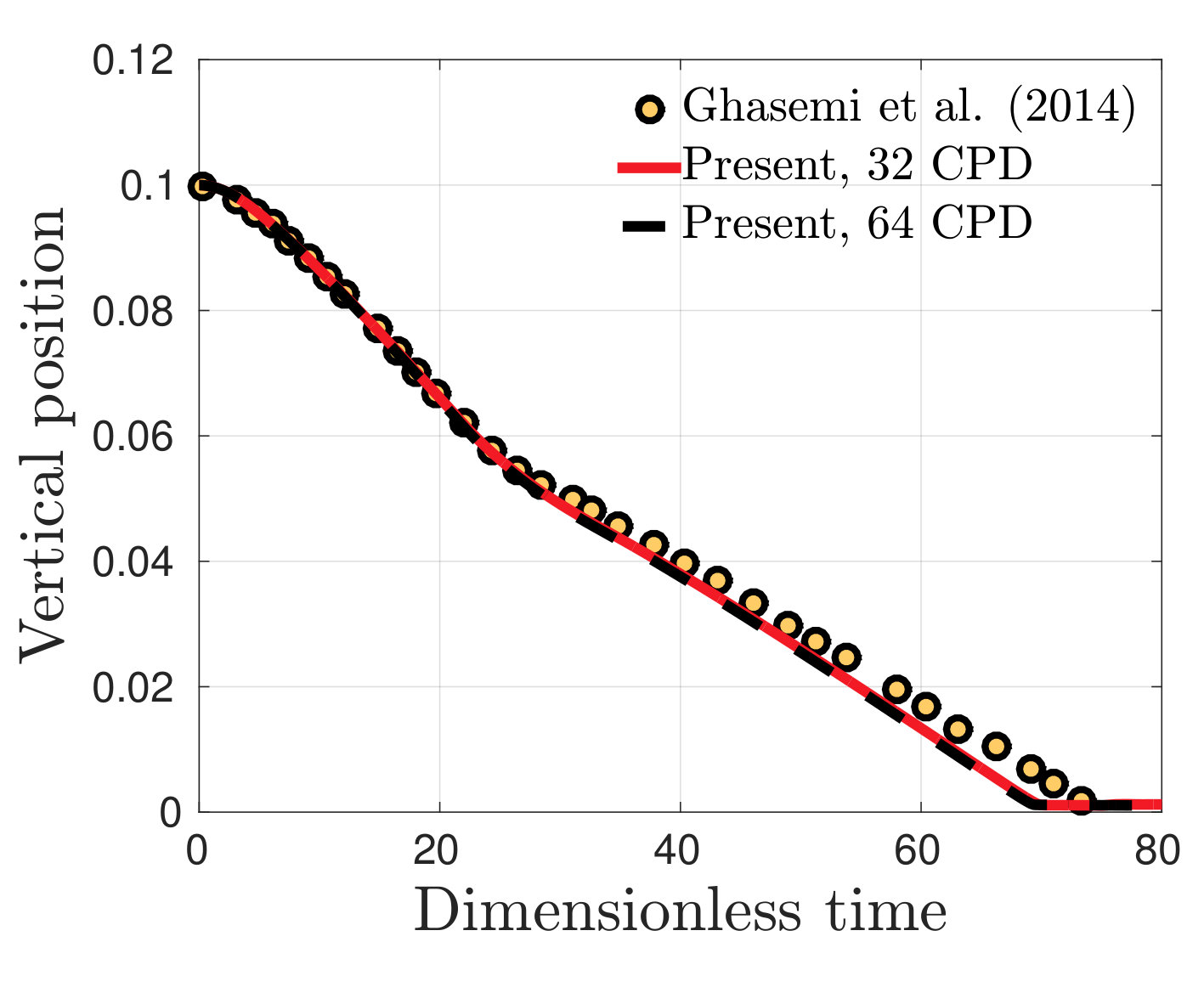 Figure 7
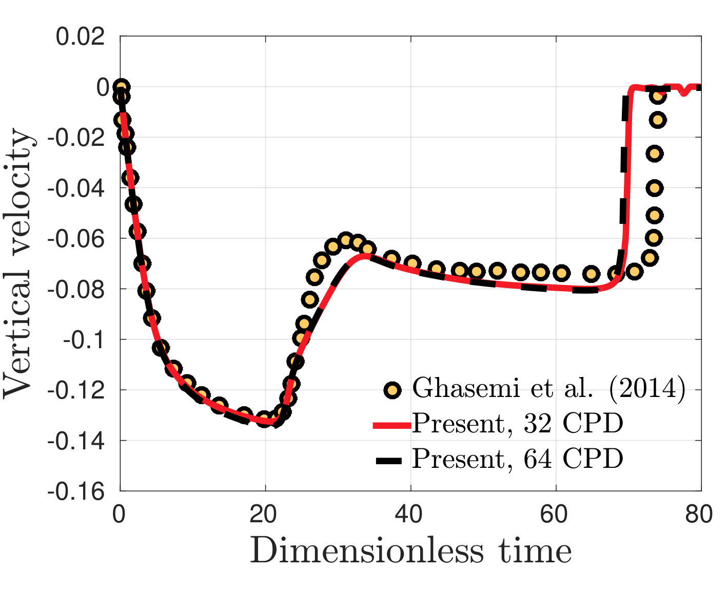 Figure 8
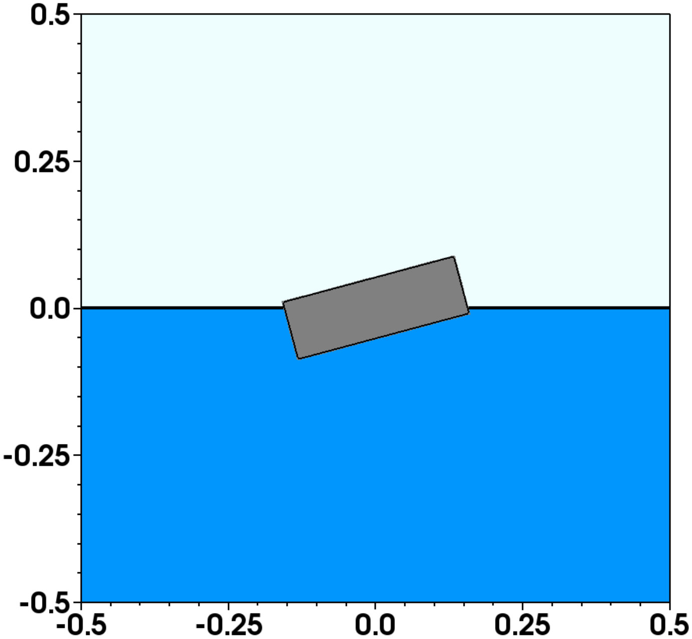 Figure 9
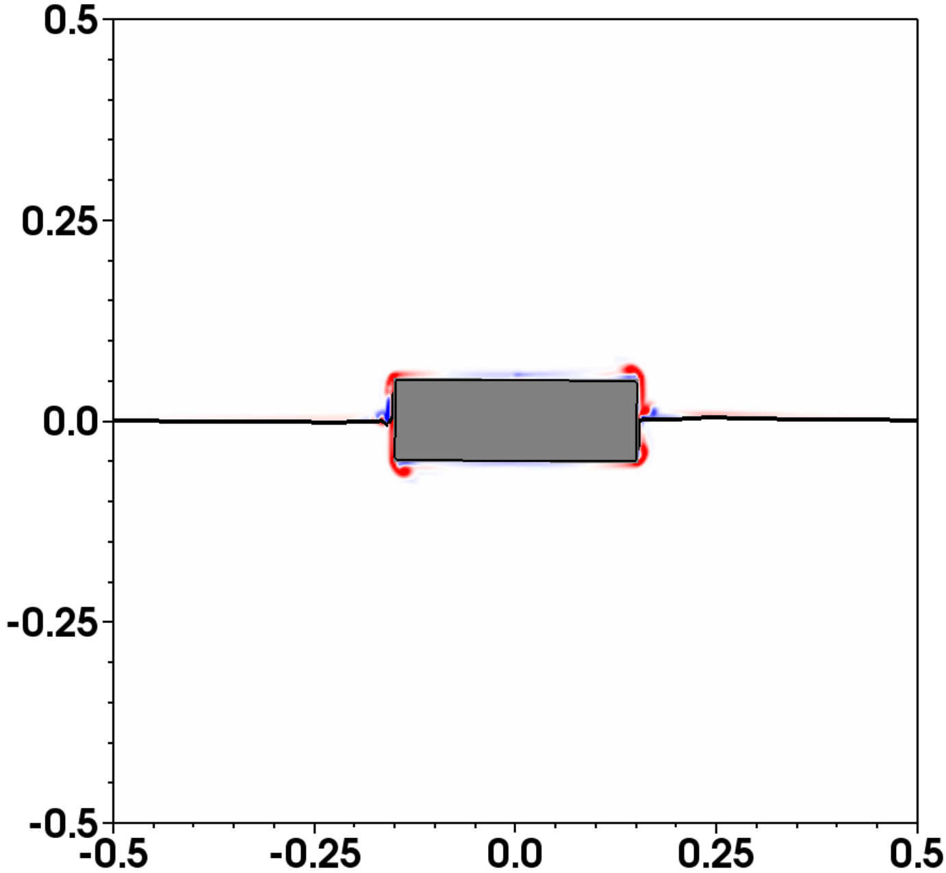 Figure 10
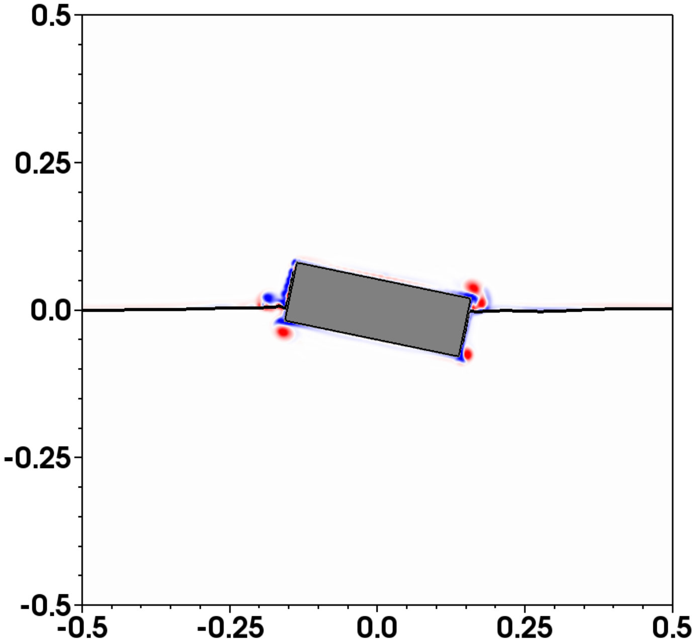 Figure 11
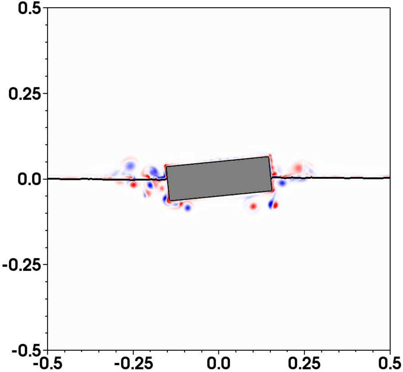 Figure 12
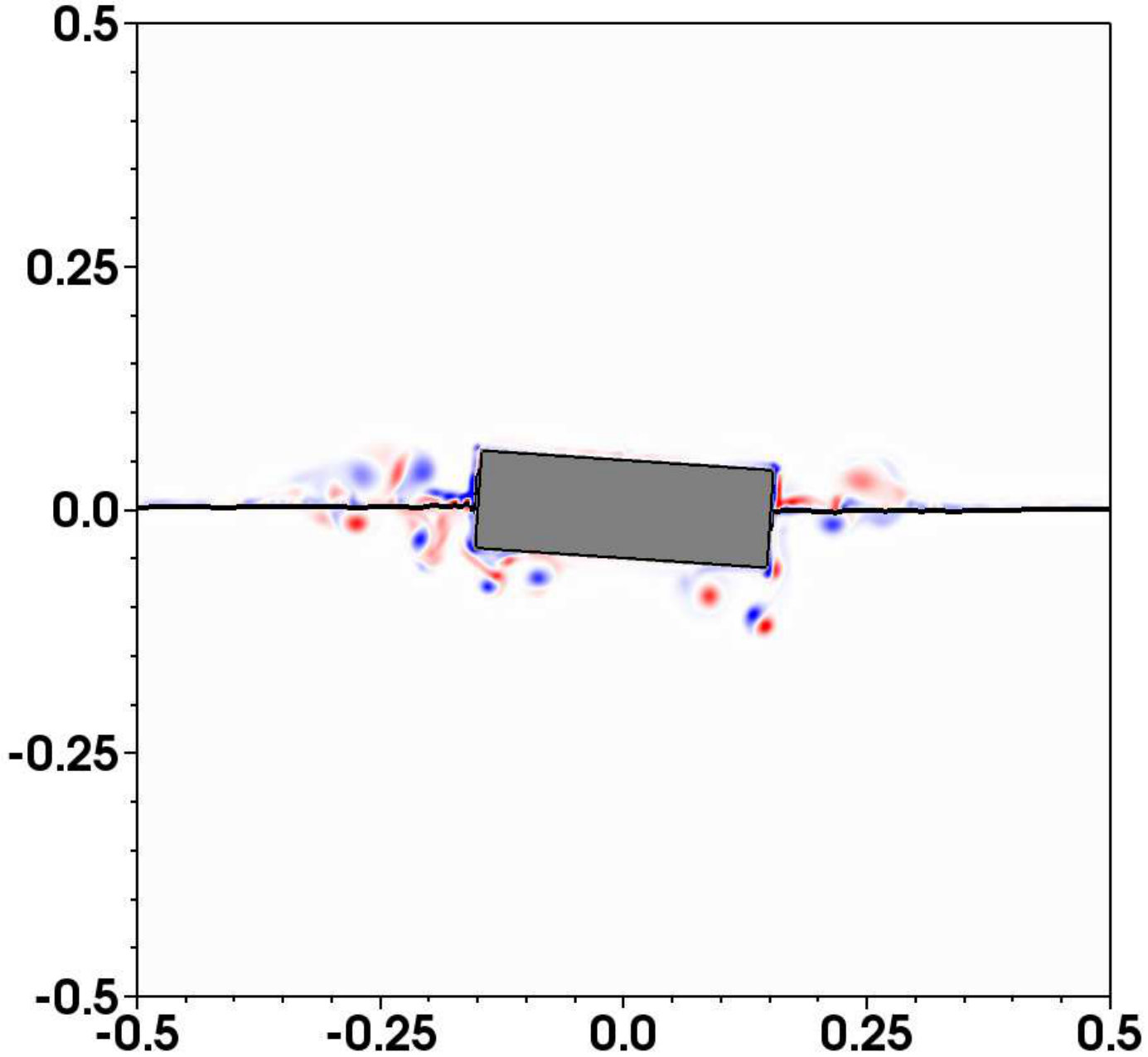 Figure 13
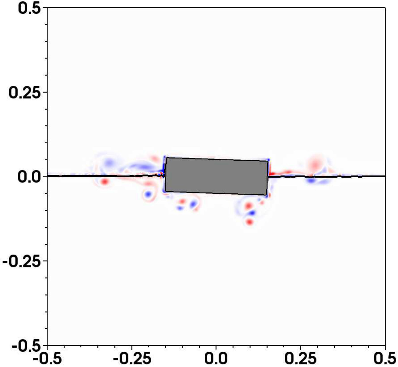 Figure 14
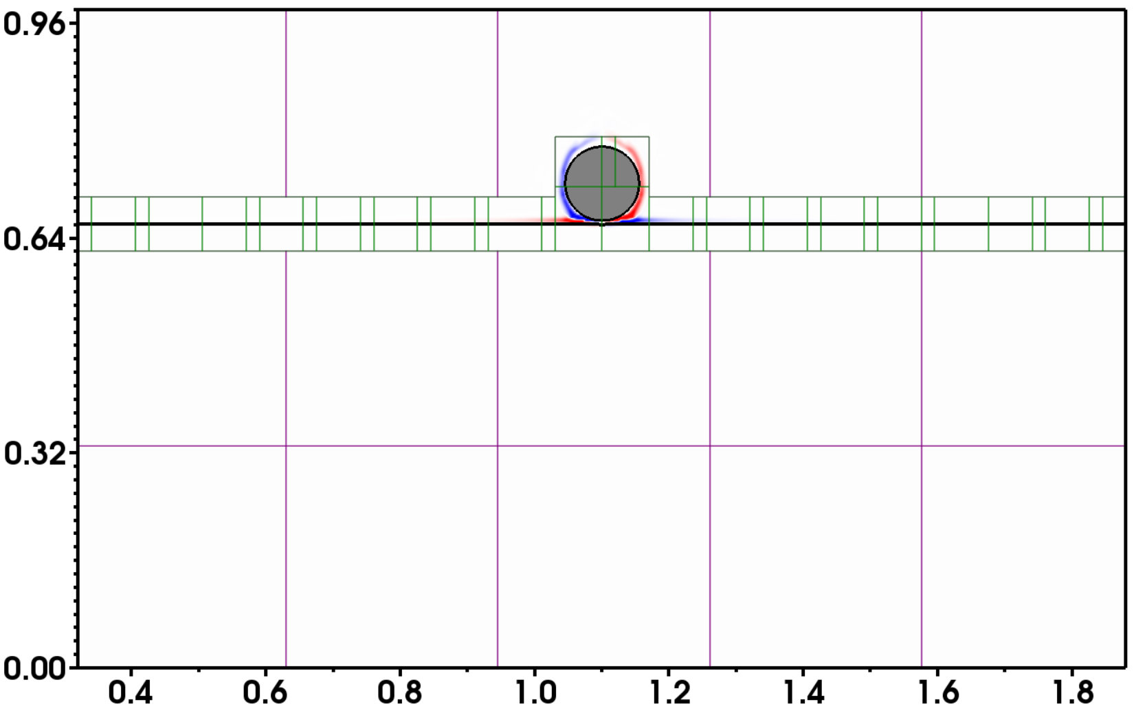 Figure 15
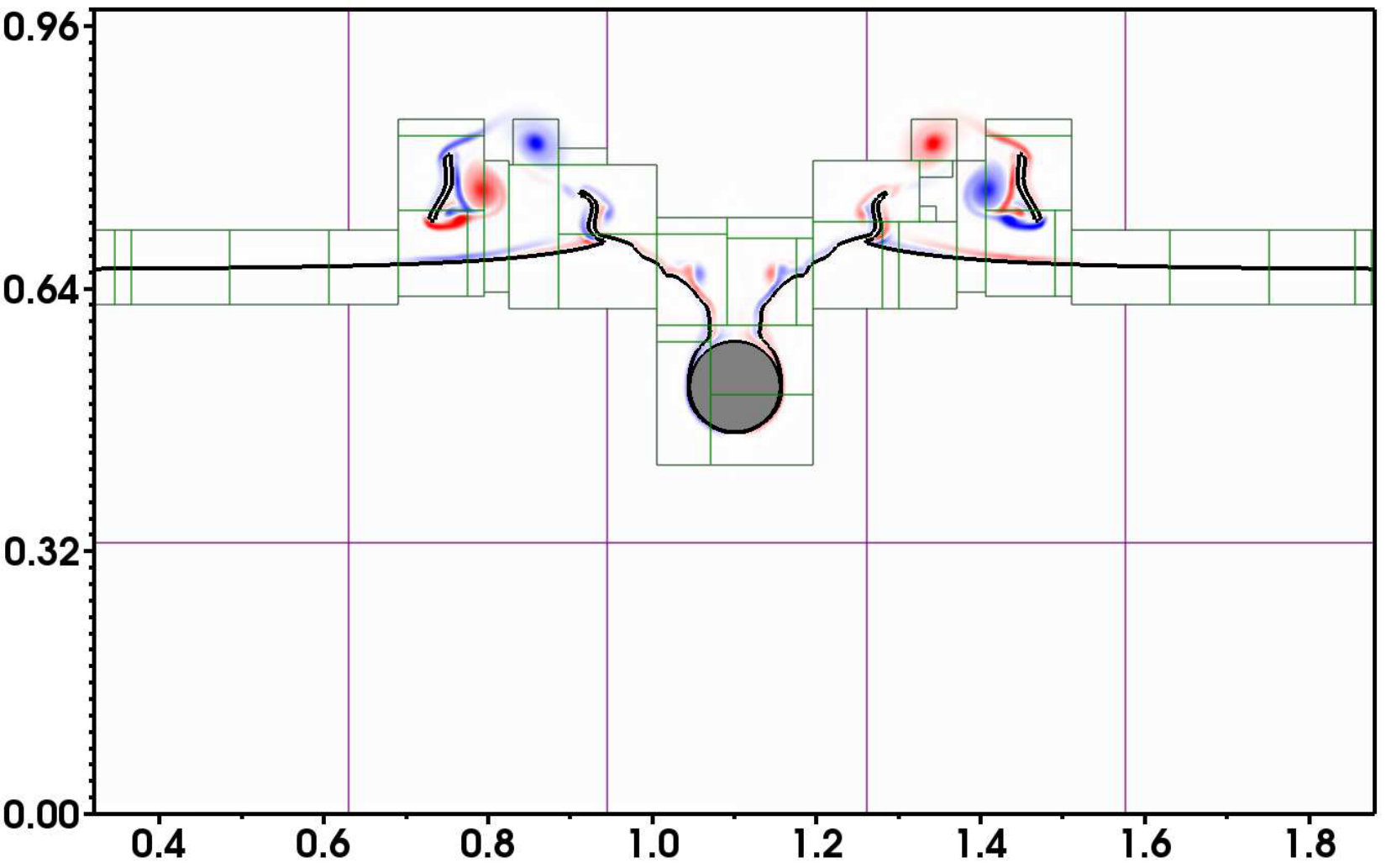 Figure 16
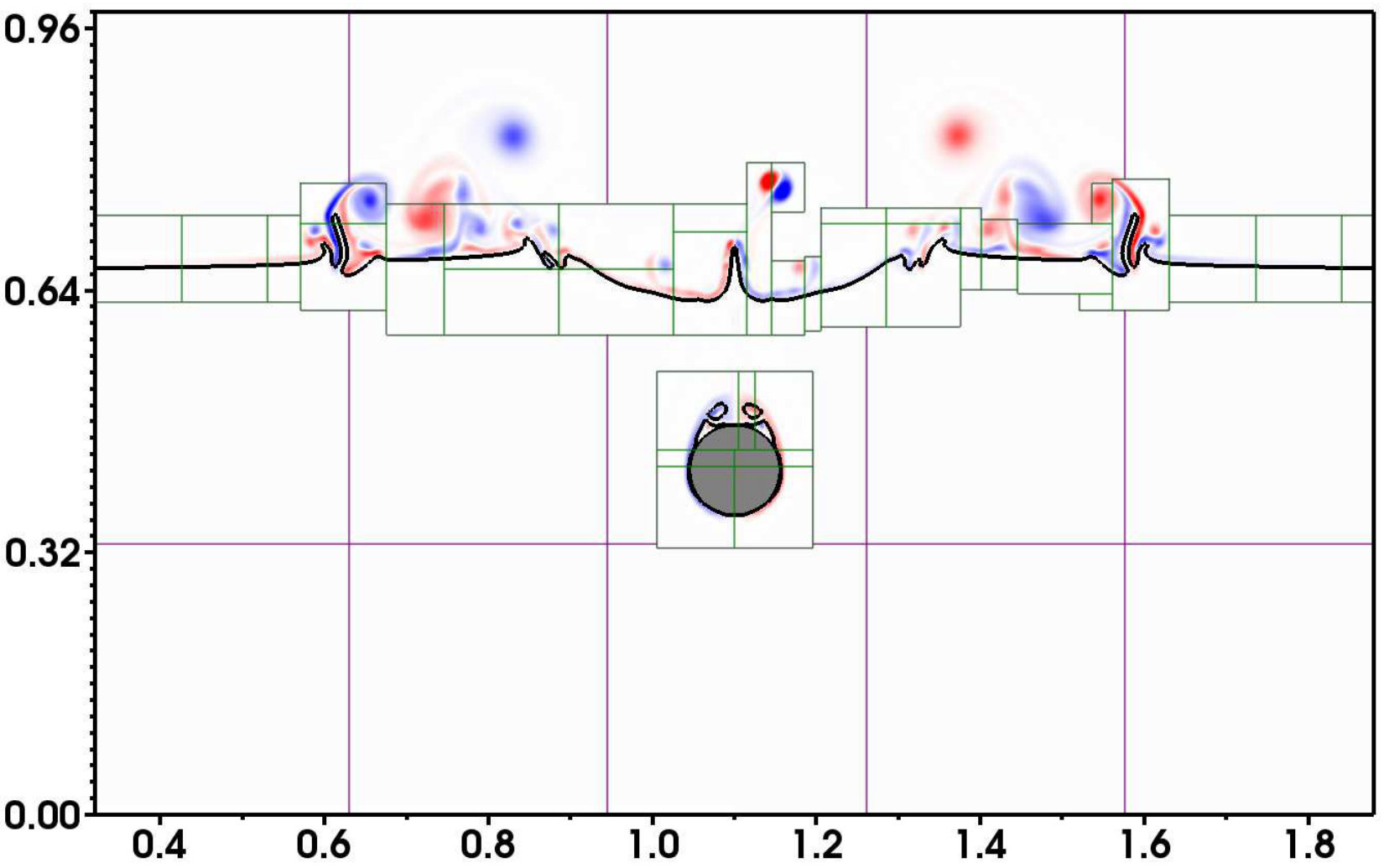 Figure 17
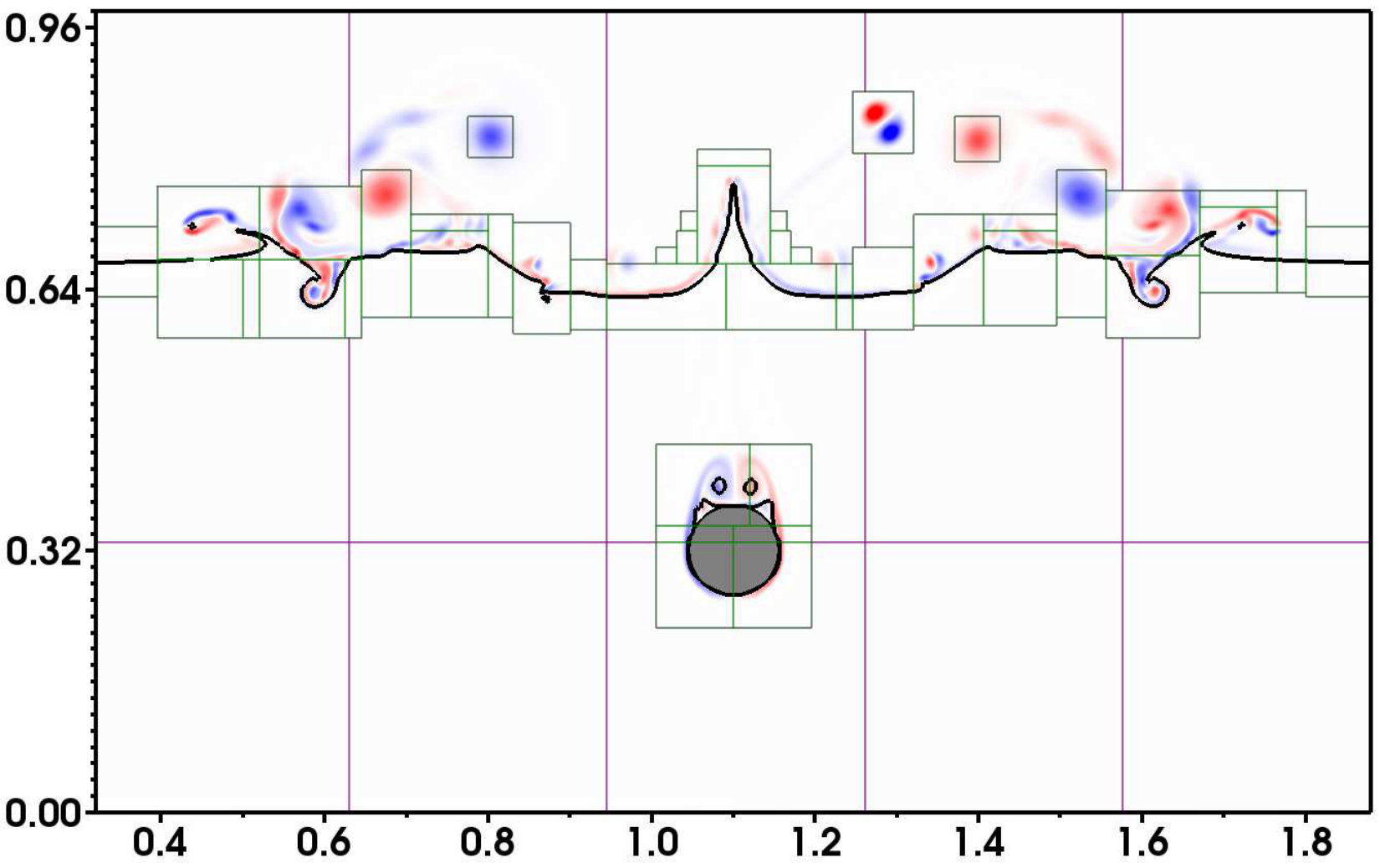 Figure 18
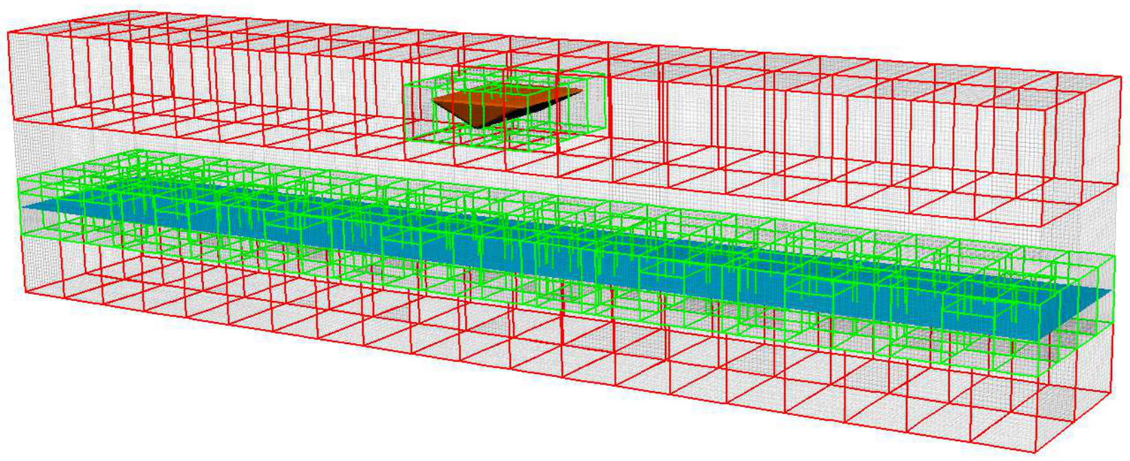 Figure 19
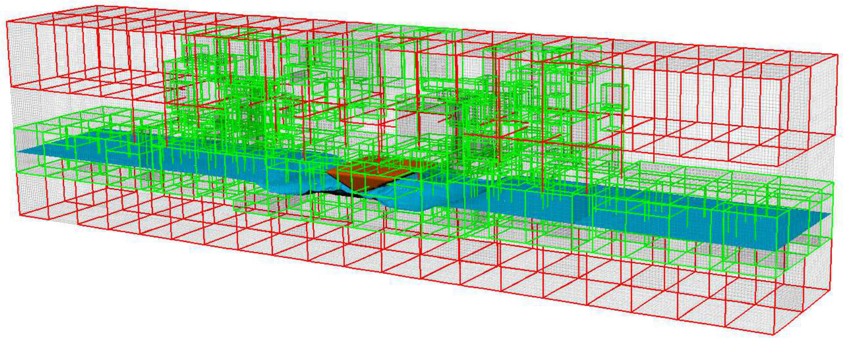 Figure 20
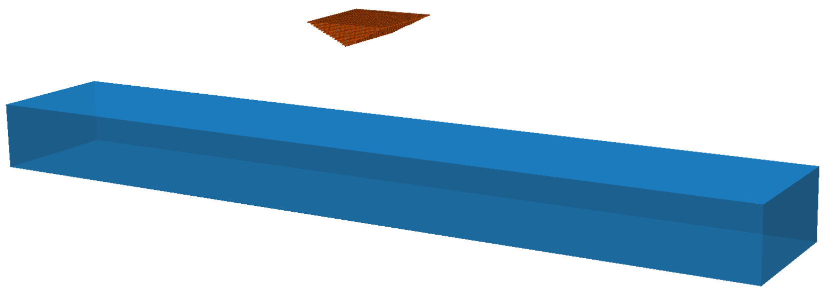 Figure 21
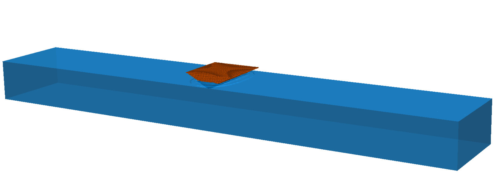 Figure 22
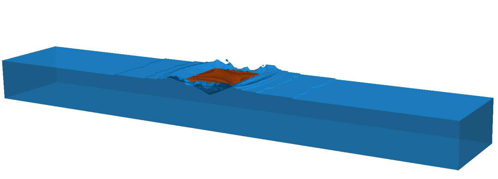 Figure 23
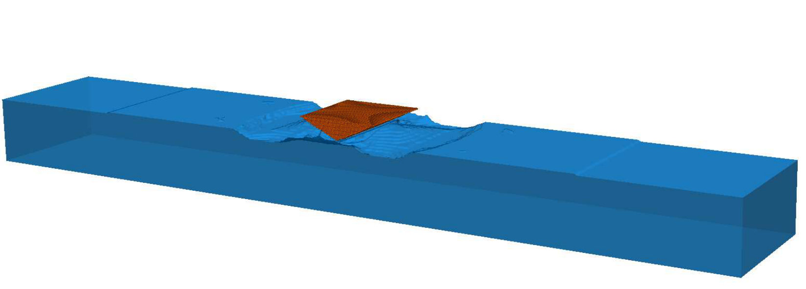 Figure 24
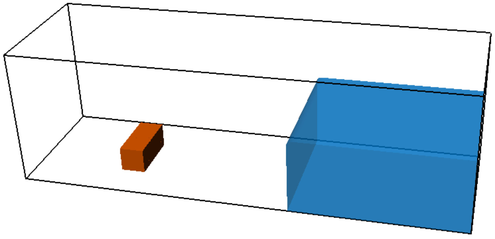 Figure 25
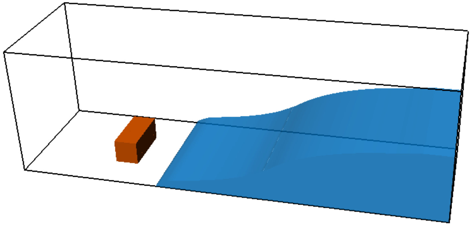 Figure 26
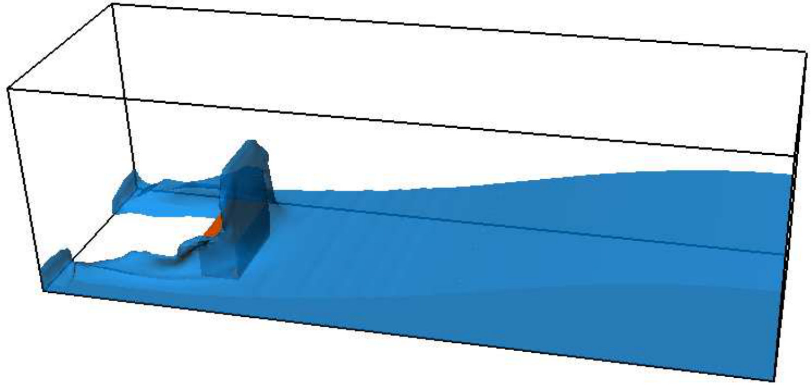 Figure 27
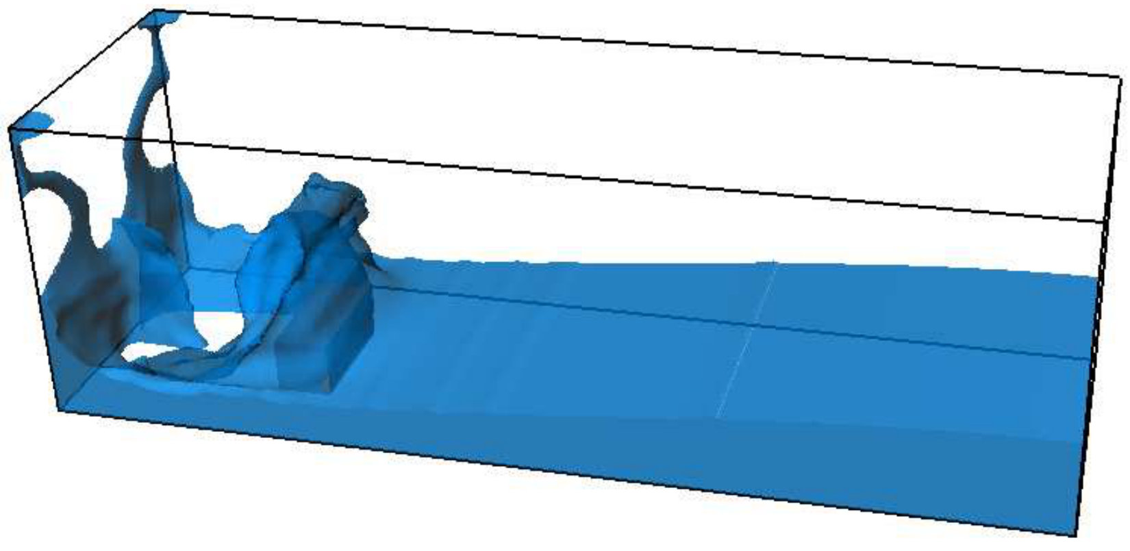 Figure 28
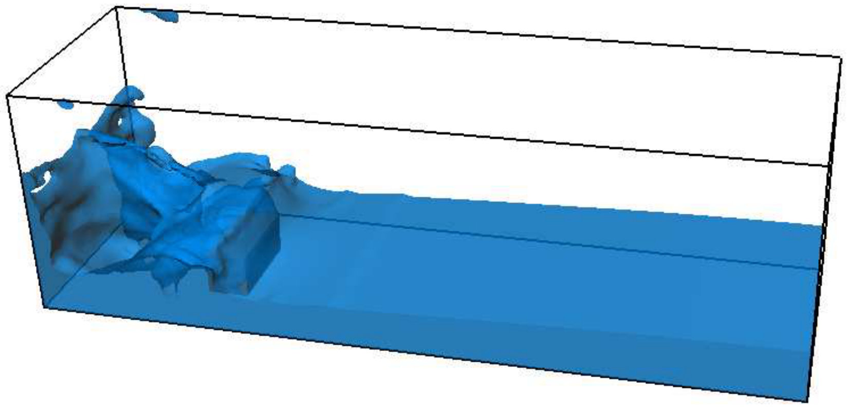 Figure 29
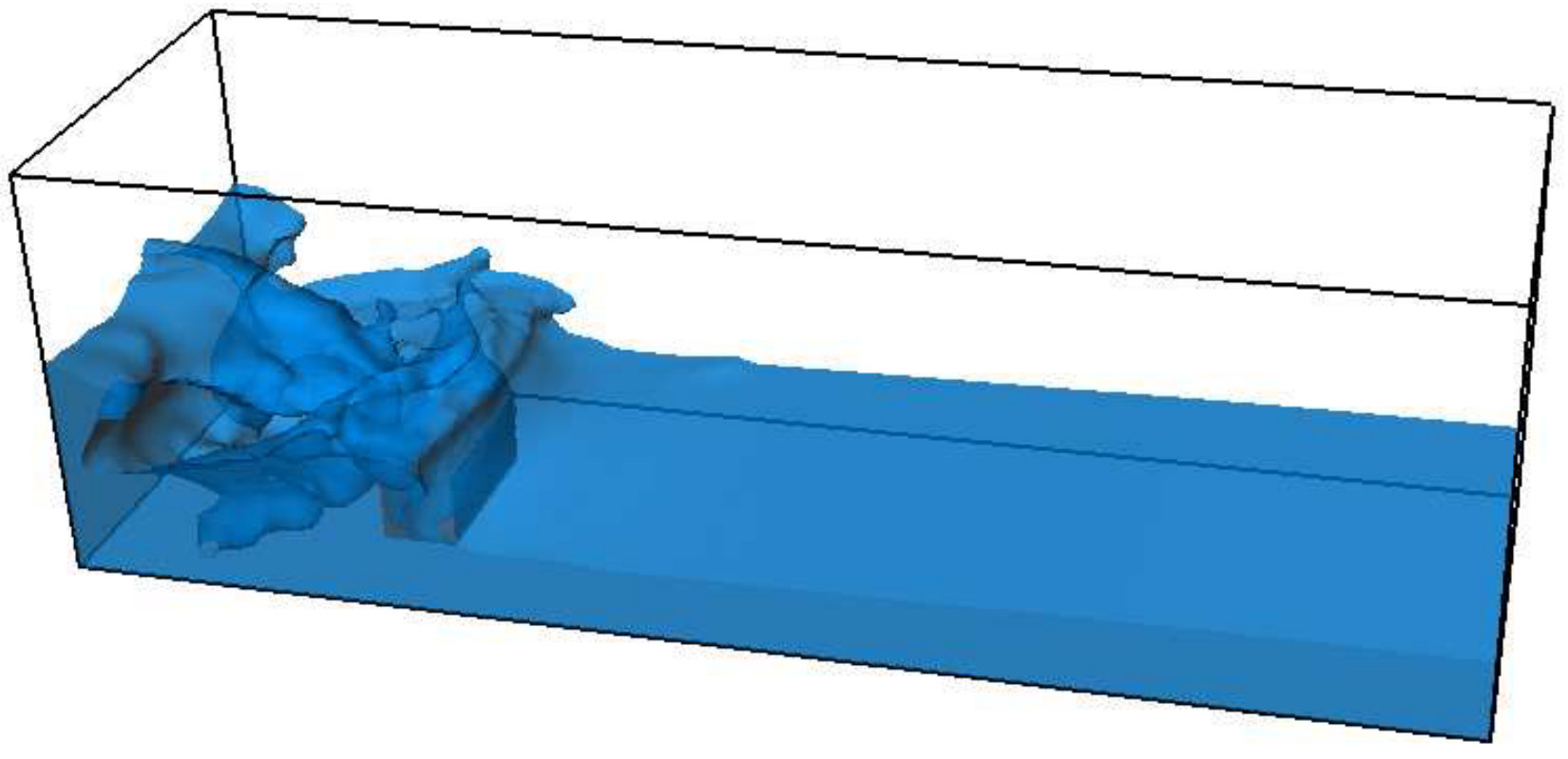 Figure 30
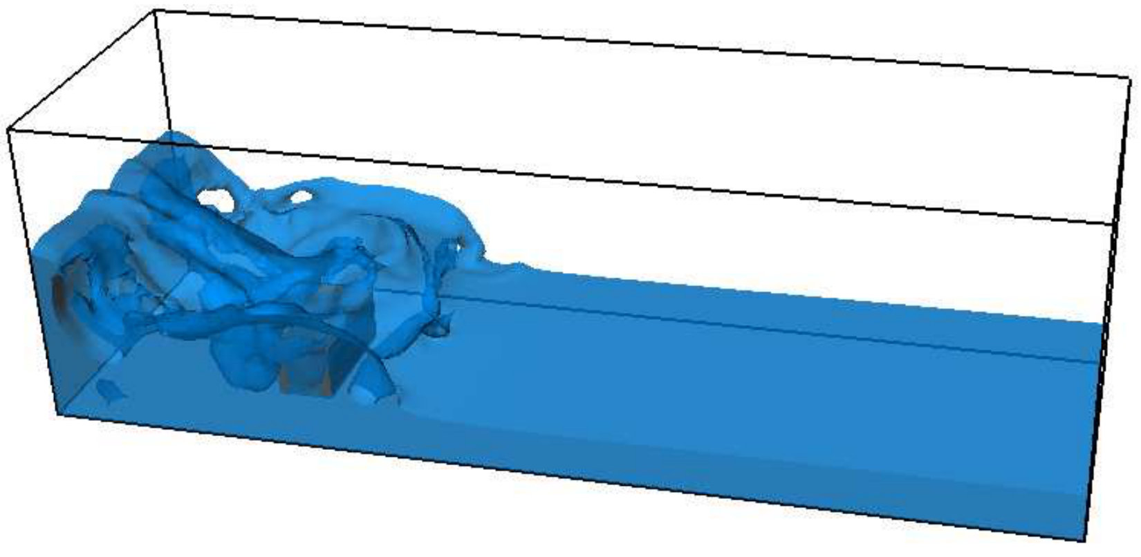 Figure 31
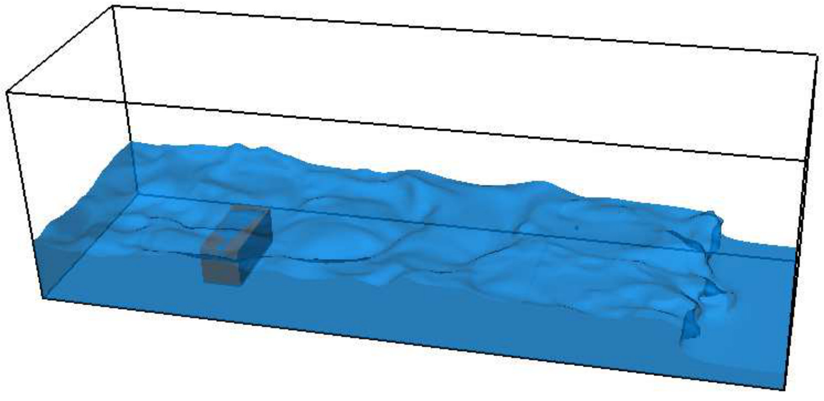 Figure 32
 Figure 33
 Figure 34
 Figure 35
 Figure 36
 Figure 37
 Figure 38
 Figure 39
 Figure 40
| Parameters | Case A | Case B | Case C |
|---|---|---|---|
| Depth () | |||
| Wave height () | |||
| Wave period () | |||
| Wavelength () | |||
| Domain size | |||
| Cells per wavelength () | |||
| Cells per wave height () | |||
| Elevation probe location () |
| Probe | Measurement | Location |
|---|---|---|
| P | Pressure | |
| P | Pressure | |
| P | Pressure | |
| P | Pressure | |
| H | Water height | |
| H | Water height |
Peer Reviews
No public reviews on file for this paper yet. If you reviewed it on a platform where reviews are public (OpenReview, ICLR, NeurIPS, ICML), you can paste yours below so the community can read it here.
Videos
No videos yet. Explain this paper in a talk, walkthrough, or lecture? Add one.
A DLM immersed boundary method based wave-structure interaction solver for high density ratio multiphase flows
Nishant Nangia
Neelesh A. Patankar
Amneet Pal Singh Bhalla
Department of Engineering Sciences and Applied Mathematics, Northwestern University, Evanston, IL
Department of Mechanical Engineering, Northwestern University, Evanston, IL
Department of Mechanical Engineering, San Diego State University, San Diego, CA
Abstract
In this paper we present a robust immersed boundary (IB) method for high density ratio multiphase flows that is capable of modeling complex wave-structure interaction (WSI) problems arising in marine and coastal engineering applications. The IB/WSI methodology is enabled by combining the distributed Lagrange multiplier (DLM) method of Sharma and Patankar (2005) [1] with a robust level set method based multiphase flow solver. The fluid solver integrates the conservative form of the variable-coefficient incompressible Navier-Stokes equations using a hybrid preconditioner and ensures consistent transport of mass and momentum at a discrete level. The consistent transport scheme preserves the numerical stability of the method in the presence of large density ratios found in problems involving air, water, and an immersed structure. The air-water interface is captured by the level set method on an Eulerian grid, whereas the free-surface piercing immersed structure is represented on a Lagrangian mesh. The Lagrangian structure is free to move on the background Cartesian grid without conforming to the grid lines. The fluid-structure interaction (FSI) coupling is mediated via Peskin’s regularized delta functions in an implicit manner, which obviates the need to integrate the hydrodynamic stress tensor on the complex surface of the immersed structure. The IB/WSI numerical scheme is implemented within an adaptive mesh refinement (AMR) framework, in which the Lagrangian structure and the air-water interface are embedded on the finest mesh level to capture the thin boundary layers and the vortical structures arising from WSI. We use a well balanced gravitational force discretization that eliminates spurious velocity currents in the hydrostatic limit due to density variation in the three phases (air, water and solid). We also show that using a non-conservative and an inconsistent fluid solver can lead to catastrophic failure of the numerical scheme for large density ratio variations that are prevalent in WSI applications. An effective wave generation and absorption technique for a numerical wave tank is presented and used to simulate a benchmark case of water wave distortion due to a submerged structure. The numerical scheme is tested on several benchmark WSI problems from numerical and experimental literature in both two and three dimensions to demonstrate the applicability of the IB/WSI method to practical marine and coastal engineering problems.
keywords:
fluid-structure interaction , adaptive mesh refinement , fictitious domain method , distributed Lagrange multipliers , numerical wave tank , Stokes wave
1 Introduction
Wave-structure interaction phenomena are critical design considerations for marine engineers to ensure the safe operability of coastal and offshore structures. In marine and coastal engineering applications, complex floating structures, such as floating oil platforms, wave energy converter (WEC) devices, and foundations of offshore wind turbines, are subject to wave loading, wave run-up, wave scattering, and wave breaking effects, which can severely damage or affect the performance of these structures.
Recently, development of marine renewable energy has received renewed interest within the scientific community due to fluctuating oil prices and the negative impact of fossil fuels on the environment. It is estimated that 2.11 0.05 TW of coastal wave energy is available globally, with equal amounts in the Northern and Southern hemispheres [2]. Simulations of WECs can help increase their power extraction capacity by interrogating the underlying physics. However, many existing numerical models of WECs are based on simplified flow physics, i.e. by assuming inviscid potential flow equations that are mostly linear [3, 4] or weakly nonlinear [5, 6]. Viscous drag in such models is generally accounted for by using Morison’s equation [7], which is valid only for slender offshore structures. Moreover, Morison’s equation has been obtained empirically from experimental measurements for limited wave conditions and is not valid over all flow regimes [8, 9]. Therefore, these methods cannot handle free-surface and wave breaking effects around the structure, which are highly nonlinear in nature. Neglecting realistic sea or ocean conditions can lead to suboptimal design for WEC devices. Fully-resolved wave-structure interaction simulations of WECs are closer to reality as they model all three phases, but are considerably costlier than potential flow models in turnaround time.
Traditionally, fluid-structure interaction (FSI) problems involving the full incompressible Navier-Stokes (INS) system of equations have been modeled by using Arbitrary Lagrangian-Eulerian (ALE) methods [10] on body conforming grids. The main advantage of an ALE-like approach is that the boundary conditions on the fluid-structure [10] or the fluid-fluid [11] interface can be satisfied exactly. For single-phase FSI applications, ALE methods can be used to obtain high-resolution results, albeit at the cost of frequent re-meshing of the entire computational domain due to the structural displacement [12]. However for WSI applications where the air-water interface undergoes non-smooth and non-continuous topological changes due to wave-breaking processes, the application of ALE methods is not practical.
To overcome these limitations, fictitious domain [13, 1] or immersed boundary (IB) methods [14], combined with level-set [15] or volume of fluid (VOF) approaches [16] are gaining popularity for both single phase FSI applications and multiphase FSI applications [17, 18, 19, 20, 21, 22]. There are two major implementation categories of the IB method — diffuse and sharp. In the diffuse IB approach, the fluid equations are extended inside the structure domain so that regular and fast Cartesian solvers can be used to solve the INS equations everywhere in the computational domain. An additional body force is applied in the structure domain, which is conveniently represented on a Lagrangian mesh to constrain the motion of the fluid occupying the solid region as a rigid body motion. The most efficient way to compute the FSI body force is through distributed Lagrange multipliers (DLM), a method pioneered by Patankar et al. [13]. A fractional time stepping approach is used to impose the DLM-based rigidity constraint, which is suitable for moderate to high Reynolds number flows [1, 23]. For zero Reynolds number Stokes flow, the DLM or constraint force needs to be computed simultaneously by solving an extended saddle point system, along with fluid velocity and pressure degrees of freedom. This is because Stokes flow is a purely elliptic system describing a force equilibration process and any fractional time stepping scheme introduces a large numerical error in its solution. Kallemov et al. [24] and Usabiaga et al. [25] describe an efficient preconditioner for the monolithic fluid-DLM solver. The FSI coupling for diffuse IB methods is mediated via Peskin’s regularized delta functions, in which the Lagrangian DLM force is spread onto the background Eulerian grid and the fluid velocity is interpolated onto the Lagrangian mesh. The use of regularized delta functions smears the fluid-structure interface over a few grid cells (according to the delta function support), which makes the interface diffuse rather than keeping it sharp. In this work we use an efficient fractional time stepping, diffuse DLM approach to model WSI. Sharp IB methods, on the other hand, imposes the velocity of the fluid-structure interface at the nearby “IB nodes”. This is achieved by fitting a spatial polynomial (linear or quadratic) through the solid interface and fluid nodes. The INS equations are solved only at the fluid nodes, with the IB nodes acting as velocity boundary conditions. The velocity and pressure values for the interior solid nodes are zeroed-out during the solution procedure, which then creates “punctured” domain effects. The most notable sharp IB method implementations and their extensions have been carried by Borazjani et al. [26], Mittal et al. [27], Udaykumar et al. [28], and Tseng and Ferziger [29].
There are several advantages and disadvantages to both diffuse and sharp IB methods. For example, diffuse IB methods permit a continuous solution of velocity and pressure in the entire domain, which eliminates “spurious force oscillations” (SFO) in the time histories of the integrated drag and lift quantities for the moving immersed bodies. In contrast, spurious force oscillations are an outstanding issue for the sharp IB methodology because of the punctured domain effect [30, 31, 22]. Since the solution is continuous throughout the domain for diffuse IB methods, there are no issues with “fresh” and “dead” fluid cells when the structure changes it location in the domain, which is an challenging issue for sharp IB methods. Diffuse IB methods also allow for an implicit coupling of the fluid and structure domains without requiring hydrodynamic stress tensor computations on the (possibly complex) surface of the immersed structure [32]. In contrast, sharp IB methods compute pointwise hydrodynamic forces on the immersed surface and often require several fluid and structure solver iterations to converge to a stable solution within a single time step [18, 33]. The main disadvantage of diffuse IB methods is the smearing of the fluid-structure interface over few grid cells, which reduces the accuracy of the solution near the interface. The order of accuracy for diffuse IB methods is generally between one and two; the former for non-smooth and the latter for sufficiently smooth FSI problems. In contrast, sharp IB methods retain full second-order accuracy by sharply resolving the fluid-structure interface. Diffuse IB methods are also known to produce non-smooth pointwise hydrodynamic stress on the immersed surface even though the net hydrodynamic force and torque are smooth and SFO-free. This issue can however be mitigated by interpolating the hydrodynamic stress sufficiently far away from the fluid-structure interface. The lack of geometric information for the immersed surface also makes the implementation of wall functions required for turbulence modeling difficult for diffuse IB methods. For sharp IB methods, application of Robin-type boundary conditions and implementing wall functions is quite natural. The SFO in sharp IB methods can be mitigated by increasing the grid resolution and using larger time steps. However, very refined meshes can make the simulations extremely expensive and the use of large time steps can make them unstable unless fully implicit time stepping schemes are used for the INS equations. The demarcation of grid nodes into “IB nodes”, “fluid nodes” and “solid nodes” is a computationally taxing task as well and a novice procedure to reconstruct the IB node velocity (from interface and fluid nodes) can lead to numerical instabilities for certain geometric configurations of the interface relative to the background Cartesian grid [33, 29, 27]. We remark that in spite of the aforementioned shortcomings of the diffuse and sharp IB methods, both have been applied successfully to solve complicated engineering problems. Combined with level set or volume of fluid methods that can capture the air-water interface on Eulerian grids, these IB methods allow for an efficient solution of topologically complex WSI problems.
An issue that is unique to WSI or two-phase multiphase flows is the presence of highly contrasting density ratios in the computational domain. High density ratio multiphase flows are known to develop numerical instabilities whenever convection is the dominant physical process [22, 34, 35, 36, 37, 19, 38, 39]. Recently the multiphase community (including us) has proposed several stabilizing remedies for convection-dominated, high density ratio multiphase flows, for solvers based on both volume of fluid and level set methods [34, 35, 19]. The underlying cause of the instability is the inconsistent transport of mass and momentum at a discrete level. In this work we achieve a consistent transport of mass and momentum by solving an additional mass balance equation using a strong-stability preserving Runge-Kutta (SSP-RK3) integrator [40]. The mass flux that updates the density variable is also used to construct a discrete convective operator for the momentum equation. This necessarily requires solving the conservative form of the mass balance and momentum equations. The strong coupling between (discrete) mass and momentum convective operators preserves the stability of the numerical scheme for density ratios as high as . Our multiphase flow solver is based on the level set method, which makes the implementation of the proposed IB/WSI methodology relatively easier (than VOF methods) on locally refined meshes. We employ a hybrid preconditioner that solves the velocity and pressure degrees of freedom simultaneously, i.e., we do not use a projection-method (which is an operator-splitting approach) to solve the INS equations [41]. Only the distributed Lagrange multipliers for the FSI coupling are imposed via operator-splitting. For computational efficiency the air-water interface and the immersed structure are resolved on the finest mesh level, whereas the rest of the computational domain is resolved on progressively coarser grids. Therefore, we are able to capture important flow features at a substantially reduced computational cost, especially in 3D. Since we extend the fluid equations inside the solid domain and since the density of the structure is different than surrounding fluid (almost always heavier than air for WSI applications), the gravitational body force can produce spurious velocity currents near the fluid-structure interface for certain cases. Similarly, due to the density contrast of air and water, spurious velocity currents can also form near the air-water interface. In this work we employ a well-balanced gravity force discretization that eliminates such spurious currents near the air-water-solid interface even in the hydrostatic limit. Section 8.4 provides a numerical example that highlights this problem and shows the numerical “fix”.
The remainder of the paper is organized as follows. We first introduce the continuous and discrete system of equations in Secs. 2 and 3, respectively. Next we discuss the solution methodology in Sec. 4. Section 5 comments on the well-balanced gravity force implementation and Sec. 8.4 presents the corresponding numerical example. Software implementation is described in Sec. 6. Section 7 describes the implementation of a numerical wave tank based on the level set method, and demonstrates the interaction of a Stokes second-order wave in the presence of a submerged structure. Finally, more complicated three-phase flow examples that demonstrate the applicability of the proposed IB/WSI methodology to simulate free-surface piercing and floating structures are presented in Sec. 8. We also contrast the consistent results from the conservative flow solver against the unstable results obtained from an inconsistent and non-conservative flow solver to highlight the importance of consistent mass and momentum transport for practical WSI applications. Wherever possible, simulation results from locally refined grids are presented.
2 The continuous equations of motion
2.1 Multiphase constraint immersed boundary formulation
We begin by stating the governing equations for a multiphase fluid-structure system occupying a fixed region of space , for or spatial dimensions. In the immersed boundary formulation, a fixed Eulerian coordinate system is used to describe the momentum equation and divergence-free condition for both the fluid and structure. It is convenient to employ a Lagrangian description of the immersed body configuration, in which denotes the fixed material coordinate system attached to the structure and is the Lagrangian curvilinear coordinate domain. The position of the immersed structure occupying a volumetric region at time is denoted by . In contrast with the previous formulation of the DLM or constraint immersed boundary method [23], we allow for a spatially and temporally varying density and dynamic viscosity , implying that the structure can be heavier or lighter than the surrounding fluids. Hence, the equations of motion for the coupled fluid-structure system in conservative form are
[TABLE]
Eqs. (1) and (2) are the incompressible Navier-Stokes momentum and continuity equations written in Eulerian form, in which is the velocity, is the pressure, and is the Eulerian constraint force density, which is non-zero only in the structure region. The gravitational acceleration is denoted by , and is the continuum surface tension force. The interactions between Eulerian and Lagrangian quantitates are facilitated by Dirac delta function kernels, in which the -dimensional delta function is . Eq. (3) converts the Lagrangian force density into an equivalent Eulerian density , in an operation called force spreading. Eq. (4) determines the physical velocity of each Lagrangian material point from the background Eulerian velocity field in an operation called velocity interpolation. This ensures that the immersed structure moves according to the local value of the velocity field (Eq. (5)), and thus the no-slip condition is satisfied at fluid-solid interfaces. Using short-hand notation, the force spreading operation is denoted by , in which is the force-spreading operator and the velocity interpolation operation is denoted by , in which is the velocity-interpolation operator. It can be shown that if and are taken to be adjoint operators, i.e. , then the Lagrangian-Eulerian coupling conserves energy [14].
The specific rigidity constraint imposed within the structure domain, written in Lagrangian form, is given by
[TABLE]
which states that the body has zero deformation rate and must undergo a rigid body motion [13]. In the present work, we compute a discrete approximation to the constraint force , although a numerical method that enforces this constraint exactly for a range of Reynolds numbers (including zero Reynolds number Stokes flow) has been described by one of us in [24, 25].
Note that the momentum equation (Eq. (1)) can also be cast to an equivalent non-conservative form. However, it has been shown that direct discretization of the non-conservative form can lead to numerical instabilities for high density ratio multiphase flows [36, 37, 38, 39, 34]. The differences between the conservative and non-conservative flow solvers will be discussed in later sections.
2.2 Interface tracking for material properties
Next, we describe the governing equations for tracking and transporting material properties. Suppose a liquid of density and viscosity occupies a region , while a gas of density and viscosity occupies a region . The codimension- interface between these two fluids is denoted by can be tracked as the zero contour of a scalar function , which is the so-called level set function [15, 42, 43],
[TABLE]
Level set methods are particularly well-suited for tracking liquid-gas interfaces undergoing complex topological changes and are relatively simple to implement in both two and three spatial dimensions, and on locally refined meshes. It is also useful to define an additional level set function to track the boundary of the immersed structure . Using this auxiliary field, the density and the viscosity in the solid region can be readily prescribed in the Eulerian regions occupied by the solid . Both level set functions are passively advected by the incompressible fluid velocity, which in conservative form reads
[TABLE]
The material properties including density and viscosity in the three phases are determined as a function of these two scalar fields by
[TABLE]
The discretized form of Eqs. (10) and (11) are defined in Section 4.1 using regularized Heaviside functions.
One particularly useful level set function is the signed distance function, which can be prescribed as initial conditions to Eqs. (8) and (9)
[TABLE]
However, we note that and generally will not remain signed distance functions under advection by Eqs. (8) and (9). A reinitialization or redistancing procedure is used to maintain the signed distance property at every time step. When the fluid properties are determined from the level set fields, we need initial conditions for and but not for or .
3 Spatial discretization
This section describes the discrete form of the governing equations for the coupled fluid-structure system. Eulerian quantities are discretized on a staggered Cartesian grid, whereas Lagrangian quantities are approximated on a collection of immersed markers that can be arbitrarily positioned on the grid. A regularized version of the Dirac delta function is used to facilitate the velocity interpolation and force spreading operations. Therefore, we are not employing a body-conforming mesh to the fluid-structure interface since the structure markers need not conform to the Eulerian grid.
Throughout this section, we describe the discretization for spatial dimensions; the discretization in two spatial dimensions is analogous. For simplicity, we describe the case for which there is no local grid refinement in the domain, although this is not a limitation of the present formulation. Details on adaptive mesh refinement are delegated to Sec. 3.4. Finally, we note that evaluating the discrete operators described in this section near boundaries of the computational domain and locally refined mesh boundaries requires the specification of adjacent “ghost” cells. For more details on the treatment of boundary conditions and coarse-fine interfaces, we refer readers to [23, 34, 44, 45].
3.1 Eulerian discretization
We employ a staggered grid discretization for quantities described in the Eulerian frame. A Cartesian grid covers the physical, rectangular domain with mesh spacing , , and in each direction. Without loss of generality, we assume that the bottom left corner of the domain is situated at the origin . Therefore, each cell center of the grid has position for , , and . For a given cell , is the physical location of the cell face that is half a grid space away from in the -direction, is the physical location of the cell face that is half a grid cell away from in the -direction, and is the physical location of the cell face that is half a grid cell away from in the -direction. The pressure degrees of freedom are approximated at cell centers and are denoted by , in which is the time at time step . Similarly, the flow and structure level set functions are also defined at cell centers and are denoted by and , respectively.
Velocity components are staggered and defined on their respective cell faces: , , and . The components of various body forces on the right-hand side of the momentum equation (Eq. (1)) are similarly approximated on respective faces of the staggered grid. The density and viscosity are approximated at cell centers and are denoted by and . These quantities are interpolated onto the required degrees of freedom as needed [34].
Standard second-order finite differences are used to approximate spatial derivative operators and are denoted with subscripts; i.e. . The full description of these staggered grid discretizations have been recorded in various prior studies and we refer readers to [34, 41, 44, 46, 47] for more details.
3.2 Lagrangian discretization
Quantities attached to the structure are described in a Lagrangian frame on immersed markers that are free to arbitrarily cut through the background Cartesian mesh. These nodes are indexed by with curvilinear mesh spacings . An arbitrary quantity can be discretely approximated on a marker points as at time . Henceforth the position, velocity, and force of a marker point are denoted as , , and . In this work we only consider rigid bodies without any constitutive model applied in the structure domain, and therefore explicit mesh connectivity information is not needed [23]. See Fig. 1 for a sketch of the discretization in two spatial dimensions.
3.3 Lagrangian-Eulerian interaction
Finally, the transfer of quantities between the Eulerian and Lagrangian coordinate systems requires discrete approximations to the velocity interpolation and force spreading operations to be defined. We briefly summarize them here to complete the description of the spatial discretization.
3.3.1 In the interior domain
For a given fluid velocity defined on faces of the staggered grid, the discretized velocity interpolation operation for a particular configuration of Lagrangian markers (i.e. away from the physical boundary follows the standard treatment
[TABLE]
in which is a regularized version of the -dimensional Dirac delta function based on a four-point kernel function [14]. For a given force density defined on Lagrangian markers, the discretized force spreading operation reads
[TABLE]
We refer readers to [23, 14] for more details on properties and implementation of the grid transfer operations.
3.3.2 Near the physical boundary
When a Lagrangian marker is near the physical boundary, the support of the standard IB kernel extends beyond the computational domain. In this case and operators are modified to and , respectively, to satisfy the discrete adjointness property near the physical boundary. Briefly, is obtained by first filling the ghost cell values abutting the physical domain to satisfy the imposed boundary conditions (say for velocity) and then using the standard weights of the operator to interpolate onto the Lagrangian marker. The adjoint spreading operator near the boundary is obtained by first spreading to ghost (and interior) cells beyond the physical boundary and then adding back values to the interior cells by identifying their mirror images in the ghosted region. More details on this construction can be found in the Appendix of Kallemov et al. [24].
3.4 Adaptive mesh refinement
Some cases presented in this work make use of a structured adaptive mesh refinement (SAMR) framework to discretize the multiphase fluid-structure interaction equations. These discretization approaches describe the computational domain as composed of multiple grid levels, which is hereafter known as a grid hierarchy. Assuming uniform and isotropic mesh refinement, a grid hierarchy with levels and coarsest grid spacings , , and has grid spacings , , and on the finest grid level, in which is the integer refinement ratio between levels. Although not considered here, both the numerical method and software implementation allow for general refinement ratios.
The locally refined meshes can be static, in that they occupy a fixed region in the domain , or adaptive, in that some criteria of interest is used to “tag” coarse cells for refinement. In our current implementation, cells are refined based on two criteria: 1) if the local magnitude of vorticity exceeds a relative threshold and 2) if the flow level set function is within some threshold of zero. This ensures that the important dynamics (e.g., regions of high velocity gradients or the multiphase interfaces) are always approximated on the most resolved mesh. Additionally, we find that restricting the liquid-gas interface to the finest grid level can greatly mitigate spurious mass changes typically seen in level set methods. We also note that the immersed structure is always placed on the finest grid level, ensuring adequate accuracy near the fluid-solid interface. We refer readers to prior work by Griffith [45] for additional details on the AMR discretization methods, which includes a description of the refine and coarsen operations carried out during hierarchy regridding and a treatment of the coarse-fine interface ghost cells.
4 Solution methodology
Our strategy for solving the coupled fluid-structure interaction system of equations is similar to that of Bhalla et al. [23]. The numerical method relies on a time-splitting approach, in which we first solve the incompressible Navier-Stokes equations (Eqs. (1) and (2)) without accounting for the constraints associated with the motion of the immersed body. We then correct the velocity field to comply with the constrained Lagrangian velocity field via a projection step. This section also describes additional complexities related to the multiphase nature of the problems considered in this work.
4.1 Interface tracking and reinitialization
As described in Sec. 2.2, two level set functions are defined for the present numerical method: 1) the scalar field whose zero contour represents the liquid-air interface and 2) the scalar field whose zero contour represents the boundary of the immersed structure . The transition between different materials on the Eulerian grid can be completely described by these two level set functions. Indeed if and represent signed distance functions to their respective interfaces, we can define smoothed Heaviside functions that have been regularized over grid cells on either side of the interfaces (assuming ,
[TABLE]
in which we have assumed that the number of transition cells is the same across and . This is not an inherent limitation of the numerical method, but is true for all the cases considered in the present work. A given material property (such as or ) is then set in the whole domain using a two-step process. First, the material property in the “flowing” phase is set via the liquid-gas level set function
[TABLE]
Next, the material property is set on cell centers throughout the computational domain, taking into account the solid phase
[TABLE]
Hence the solid level set always takes precedent over the flow phase. Note that we have assumed that the liquid phase is represented by negative values and the solid phase is represented by negative values, without loss of generality.
Even if and are initially set to be the signed distance function from their respective interfaces, they are not guaranteed to retain the signed distance property under linear advection, Eqs. (8) and (9). Let denote the flow level set function following an advective transport after time stepping through the interval . The flow level set is reinitialized to obtain a signed distance field by computing a steady-state solution to the Hamilton-Jacobi equation
[TABLE]
which will yield a solution to the Eikonal equation at the end of each time step. We refer the readers to [34] for more details on the specific discretization of Eqs. (24) and (25), which employs second-order ENO finite differences combined with a subcell-fix method described by Min [48], and an immobile interface condition described by Son [49].
Since we only consider relatively simple body geometries in the present work, we can make use of the positions of the Lagrangian markers to reinitialize the structure level set function. As an example, let a volumetric sphere body with radius be made up of Lagrangian markers. At time , its center of mass can be computed as
[TABLE]
and the structure level set function can be directly recomputed as . (Note that whenever appears as a superscript, it refers to a time step number, whereas as a subscript refers to the indexing of Lagrangian particles.) For more complicated immersed bodies, one can make use of constructive solid geometry (CGS) concepts or R-functions (see Shapiro [50]) to determine analytical expressions for various signed distance functions 111R-functions tend to smooth sharp corners of geometries. We prefer CGS over R-functions wherever the former is applicable.. In the present work, we always reinitialize both level set functions every time step.
4.2 Full time stepping scheme
Next, we describe the temporal discretization over the interval for the coupled fluid-structure equations of motion. We employ cycles of fixed-point iteration per time step, with being used for all the cases in the present work. Note that appears in superscript to denote the cycle number. The full time stepping scheme consists of three major operations:
Advect the signed distance functions, obtaining and , and the cell-centered viscosity using the signed distance functions 222We first set the cell-centered viscosity and then use harmonic averaging to interpolate onto the appropriate degrees of freedom.. 2. 2.
Solve the incompressible Navier-Stokes equations, obtaining and . 3. 3.
Enforce the rigidity constraint, obtaining and the corrected fluid velocity .
At the beginning of each time step we set , with , , , , and . At the initial time step , these quantities are obtained using the prescribed initial conditions. The midpoint, time-centered approximations to these quantities are given by , , , , and . Below, we describe in detail the solution methodology for all three steps.
4.2.1 Scalar advection
The level set functions are updated by discretizing Eqs. (8) and (9), which reads
[TABLE]
in which represents an explicit piecewise parabolic method (xsPPM7-limited) approximation to the linear advection terms on cell centers. We refer the readers to [44, 51] for more details on the numerical implementation of this flux limiter. Homogenous Neumann boundary conditions for and are imposed on , using a standard ghost value treatment [46].
4.2.2 Incompressible Navier-Stokes solver: Conservative and consistent transport formulation
The incompressible Navier-Stokes equations Eqs. (1) and (2) are discretized and solved for in conservative form as
[TABLE]
in which is an explicit cubic upwind interpolation (CUI-limited) [52, 53, 54] approximation to the nonlinear convection term, and is a semi-implicit approximation to the viscous strain rate with . The above time-stepping scheme with is similar to a combination of explicit midpoint rule for the convective term and Crank-Nicolson for the viscous terms. We note that the newest approximation to viscosity is obtained via the procedure described in Eqs. (22) and (23). The newest approximation to density in Eq. (29) is obtained by solving a discretized mass update equation directly on the faces of the staggered grid from the previous time step and level set synchronized density field (obtained after averaging and onto faces). The discretized density update equation is solved using the third-order accurate strong stability preserving Runge-Kutta (SSP-RK3) time integrator [40] as follows
[TABLE]
Here is an explicit CUI-limited approximation to the linear density advection term; is either or . We distinguish , the density vector obtained via the SSP-RK3 integrator, from , the density vector that is set from the level set fields. The subscript “adv” indicates the interpolated advective velocity on the faces of face-centered control volume, and the subscript “lim” indicates the limited value (see Nangia et al. in [34] for details on obtaining advective and flux-limited fields). We remark that the density integration procedure is occurring within the overall fixed-point iteration scheme. We have found it to be crucial to use appropriately interpolated and extrapolated velocities to maintain the second-order accuracy of the INS scheme. To wit, for the first cycle (), the velocities are
[TABLE]
For all remaining cycles (), the velocities are
[TABLE]
Notice that is an approximation to , and is an approximation to . Similarly, is an approximation to , and is an approximation to . To ensure consistent transport of mass and momentum fluxes, the convective derivative in Eq. (29) is given by
[TABLE]
which uses the same velocity and density used to update in Eq (33). This is the key step required to strongly couple the mass and momentum convective operators. Results presented in Sec. 8 demonstrate that the consistent discretization is stable for practical air-water density ratio of and produce significantly more accurate results than the inconsistent discretization for realistic three phase WSI simulations.
4.2.3 Incompressible Navier-Stokes solver: Non-conservative and inconsistent transport formulation
One can directly use the face-centered density field obtained through the updated level set information, and , and integrate the INS equations from . In this scenario the time stepping scheme reads
[TABLE]
in which is an explicit CUI-limited approximation to the nonlinear convection term in non-conservative form (i.e. ) [34]. Integrating INS equations in the above manner decouples the mass and momentum advection and this results in an inconsistent transport of mass flux in the two discrete operators.
The performance of these two solvers are compared for some of the numerical examples considered in Sec. 8. In particular, we will show that the non-conservative solver is numerically unstable for highly contrasting air-water density ratios. When stable, both schemes are second-order accurate in time. The continuum surface tension [55] force is computed as a function of the flow level set field , and its treatment is described in [34].
4.2.4 Incompressible Navier-Stokes solver
We obtain the updated velocity and pressure fields by simultaneously solving Eqs. (29) and (30) (or Eqs. (39) and (40)) using the flexible GMRES (FGMRES) Krylov solver [56] preconditioned by a variable-coefficient projection method that is hybridized with a local-viscosity solver [44, 41]. The solvers have been shown to be second-order accurate in space and to converge for density and viscosity ratios of up to [34]. Unless otherwise stated, a relative convergence tolerance of is specified for the FGMRES solver, which leads to a converged solution in between and iterations for all of the cases considered here.
4.2.5 Rigid body projection
In general, the velocity field computed from the conservative (Eqs. (29) and (30)) and non-conservative (Eqs. (39) and (40)) flow solvers will not satisfy the constraints placed in the structure domain (Eq. (6)). To correct the velocity in , we carry out the following projection step [23]
[TABLE]
in which is the Eulerian constraint force that imposes the rigidity constraint. This force can be computed by spreading the Lagrangian constraint force , which is constructed using the difference between the desired body velocity and the interpolated uncorrected fluid velocity:
[TABLE]
This force is nonzero only in the structure domain. A correction of this type ensures that the fluid velocity in approximately matches that of the body’s Lagrangian velocity . Combining Eqs. (41) and (42) yields a succinct update equation for the Eulerian velocity field
[TABLE]
which is identical to the update described by Bhalla et al. [23] for neutrally buoyant (constant density) problems. In fact, we simply reuse an existing implementation [57] of the DLM or constraint immersed boundary method to carry out our multiphase FSI simulations. Note that in general, the corrected velocity field will not satisfy the discrete continuity equation, i.e. . One could apply an additional velocity projection and pressure correction step to ensure that the final velocity is divergence-free [23], but we have found that it is not necessary to obtain accurate results. As described previously [44, 34], the initial value for pressure at the start of each time step does not affect the flow dynamics nor the pressure solution at the end of the time step ; rather it serves as an initial guess to the iterative solution of the linear system.
Next, we describe a procedure to determine , which is required to compute . Since the structure is constrained to have a vanishing deformation rate tensor, the velocity of each Lagrangian marker can be decomposed as the following rigid body motion (dropping the time superscripts for now)
[TABLE]
in which and represent the linear and angular center of mass velocities, respectively, and is the radius vector pointing from the center of mass to the Lagrangian marker position. Two distinct scenarios are considered in the present work:
Fully prescribed motion:
For problems in which the motion of the body is specified as a function of time, we can directly set the Lagrangian velocity field at time step as
[TABLE]
which is then used to update the position of the Lagrangian markers
[TABLE]
This algorithm can be used to simulate one-way FSI problems such as flows past stationary objects or bodies entering or exiting fluid interfaces with constant velocity. 2. 2.
Free-body motion:
For coupled problems in which the body moves as a result of the fluid-structure interaction, we determine the Lagrangian velocity field at time step by redistributing the linear and angular momentum [13, 58, 23] in the structure domain
[TABLE]
Here, is the moment of inertia tensor, in which is the -dimensional identity tensor, and is the mass of the body. Note that since we assume a uniform density in the solid region, the contribution from cancels out in the actual implementation of Eqs. (47) and (48). Hence, buoyancy effects due to differences in the fluid and solid densities are implicitly accounted for by the multiphase fluid solver. Once the rigid body velocity components are determined, the structure’s velocity and position are updated via Eqs. (45) and (46).
We remark that the above formulation assumes that the six rigid degrees of freedom either are all fully prescribed (locked) or all undergoing free-body motion (unlocked). This is not a limitation of the implementation: we are able to mix and match which degrees of freedom are locked and unlocked. Many of the numerical examples considered in the present work make use of this flexibility. Finally, we make two interesting observations in the rigid body projection algorithm:
The fluid-structure coupling is implicit, i.e., we are not iterating back-and-forth between a fluid and a rigid body integrator. 2. 2.
We do not need to explicitly evaluate the hydrodynamic stress on the immersed structure to displace it or solve the fluid equations with internal velocity boundary conditions.
The physical reason behind this implicit coupling can be understood if we consider the hydrodynamic force as an internal force of the system, which is equal and opposite at the fluid-structure interface. This is the essence of the fast and efficient DLM method of Sharma and Patankar [1]. This makes our method computationally more efficient than certain sharp-interface IB approaches, which can require several stability-preserving FSI iterations and complex velocity and pressure reconstruction techniques at the immersed surface to compute hydrodynamic forces and moments [18, 33].
5 Prescription of solid density, viscosity and a well-balanced gravitational force
In the case of a neutrally buoyant structure within a single phase flow, the density and viscosity within is simply taken to be that of the surrounding fluid (i.e. the constant and used in the momentum equation) [23]. However, the choice of the “virtual” fluid that occupies the solid region for multiphase flow problems warrants additional discussion. Specification of and in this region is required to ensure that the linear system of equations (29) and (30) is well-posed.
For the “virtual” viscosity, we follow the recommendation of Patel and Natarajan [22] and set equal to that of the largest (most viscous) of all fluids in the problem. In our experience, this choice leads to accurate FSI simulations and reasonably fast convergence of the FGMRES solver. In cases where the object is undergoing free-body motion, e.g. a sedimenting sphere, a proper specification of the solid density is vitally important in order to capture inertia and buoyancy effects due to the structure’s weight. Hence, we must set based on the physical properties of the body we are trying to simulate.
In cases where the immersed body’s velocity is fully prescribed, we set equal to that of the largest (most dense) of all the fluids in the problem. Note that when this object is in contact with the less dense phase, the gravitational term in the momentum equation will generate spurious momentum in the solid phase. These spurious velocities will contaminate the flow field throughout the duration of simulation and lead to inaccurate results. In order to mitigate this erroneous momentum generation, we compute the gravitational body force using only the flow density field (see Eq. (22) and Fig. 2(a)). Thus for the fully prescribed kinematics case enters only in the linear operator but not as a gravitational body force in the solid region. As we showed in our previous work, the gravitational force based on is well-balanced by the pressure gradient term [34]. Hence, we in-effect recover a well-balanced gravity force for the coupled three-phase flow problem as well; we will show in Sec. 8 that no parasitic currents are generated at the air-water-structure interface in the hydrostatic limit.
6 Software implementation
The numerical algorithm described here is implemented in the IBAMR library [57], which is an open-source C++ simulation software focused on immersed boundary methods with adaptive mesh refinement. All of the numerical examples presented here are publicly available via https://github.com/IBAMR/IBAMR. IBAMR relies on SAMRAI [59, 60] for Cartesian grid management and the AMR framework. Linear and nonlinear solver support in IBAMR is provided by the PETSc library [61, 62, 63]. All of the example cases in the present work made use of distributed-memory parallelism using the Message Passing Interface (MPI) library. Between and processors were used in all the cases described here.
7 Wave-structure interaction
In this section, we demonstrate that the present numerical method is capable of modeling complex wave-structure interaction problems arising in marine and coastal engineering. We begin by describing our implementation of a numerical wave tank (NWT). Although NWTs based on VOF methods have been detailed in the literature [8, 64, 65, 66], studies based on the level set methodology are sparse [67, 20, 68]. Wave generation and wave absorption techniques for NWTs is an active area of research, and there are several strategies recommended in the literature (typically in the context of VOF methods) [65, 66]. In this work, we use a combination of Dirichlet wave generation boundary conditions and a relaxation-based wave damping procedure as our preferred choice. More specifically, by imposing inlet velocity boundary conditions based on Stokes wave theory at one end of the domain we are able to generate nonlinear water waves, which coherently propagate throughout the computational domain. By smoothly damping the traveling wave over a wavelength long region towards the opposite end, we mitigate the wave reflection and wave interference phenomena.
In Sec. 7.1, we describe some background theory required to simulate a NWT within the present computational methodology. In Sec. 7.2, we present a number of validation cases to demonstrate that the solver is able to accurately produce second-order Stokes waves. In Sec. 7.3, we investigate the problem of second-order Stokes wave interaction with a submerged trapezoid. The material properties of the liquid (gas) phase are set to be that of water (air): , , , and . The gravitational acceleration of is directed in the negative -direction for the D simulations presented in this section.
7.1 Stokes wave theory and numerics
According to second-order Stokes theory [3], the wave elevation from a mean water depth is given by
[TABLE]
in which is the peak-to-peak height of the wave, is the time period, is the angular frequency, is the wavelength, and is the wave number. The horizontal and vertical components of velocity that generate this wave profile are written as
[TABLE]
Note that in the above expressions for the theory and numerics presented in this section, we are considering a domain with bottom left corner situated at , without loss of generality. Since the water phase is represented by negative signed distance values and the free surface is initially located at , the elevation of the wave can be computed from via
[TABLE]
in which is the -coordinate of grid cell . Since represents the signed distance function to the interface, it is straightforward to show that the computed elevation will only be a function of the horizontal grid index , i.e. for all .
At the inlet (left) boundary, we impose the desired velocities Eqs. (50) and (51) as boundary conditions acting only in the liquid phase. For the normal velocity component, we compute the face-centered level set value based on the analytical elevation value along the computational boundary, . The normal velocity boundary condition is then given by , where the expression for the numerical Heaviside at the boundary reads
[TABLE]
In the above expression, represents a characteristic grid spacing for grids with unequal grid spacing in each direction, e.g. . Similarly for the tangential velocity component, the desired node-centered level set values can be computed as with corresponding Heaviside function , which are multiplied by to obtain desired boundary condition. We refer readers to [34, 44] for more details on the imposition of normal and tangential velocity boundary conditions in a staggered flow solver. Note that we are simply imposing homogenous Neumann conditions for the level set value at all domain boundaries. No-slip boundary conditions are imposed along the bottom and right boundary, while homogenous tangential velocity and zero pressure boundary conditions 333Imposition of pressure or normal traction boundary conditions is possible because of the monolithic velocity-pressure solver. are imposed at the top boundary.
In order to mitigate the reflection of waves at the right boundary, we place a damping zone at the downstream end of the computational domain from to . We follow the approach described by Jacobsen et al. [66], in which the numerical velocities and level set values are smoothly relaxed at the end of each time step via,
[TABLE]
In the above expressions, the superscript “computed” indicates the staggered grid velocity and cell-centered level set values computed from the solution methodology described in Sec. 4.2, and the superscript “target” indicates the desired analytical values representing still water of depth . Hence, , , and . The relaxation parameter is smoothly varied from , at the interface between the non-relaxed portion of the domain and the damping zone (e.g. ), to [math] at the rightmost computational boundary (e.g. ). For example at cell centers, the functional form of alpha reads,
[TABLE]
in which is the normalized horizontal coordinate varying from [math] to across the length of the damping zone. Analogous expressions are determined for and . In all of the cases considered in this section, a damping zone of length is prescribed. Next, we present various numerical examples demonstrating the accuracy of the aforementioned wave generation and damping techniques.
7.2 Validation of second-order Stokes waves propagating in a NWT
As an initial example we consider a D computational domain of size , which is occupied by initially quiescent water of depth . Air occupies the remainder of the domain from to . One grid cell of smearing is used on either side of the air-water interface and surface tension forces are neglected. The domain is discretized by a grid of size and a constant time step size of is used. The wave parameters are chosen to be , , and ; these are chosen to satisfy the required dispersion relation for (second-order) Stokes waves [3],
[TABLE]
To quantitatively assess the accuracy of the wave generation boundary conditions, the analytical and simulated elevation computed at a probe situated at , are plotted against time in Fig. 3 for three different grid sizes: , , and . As the resolution increases, the numerical simulations converge towards the theoretical elevation given by Eq. (49). The errors in maximum elevation attained over the shown time period decrease as the resolution increases, yielding a convergence rate of between grid sizes and and a convergence rate of between grid sizes and . There are approximately grid cells per wave height and grid cells per wavelength for the finest resolution case considered here, which we hereafter denote as Case A.
For our next example we consider two additional sets of wave parameters, which we denote as Case B and Case C; see Table 1 for a full specification of all three cases. These parameters are chosen such that they satisfy the dispersion relation Eq. (58) and occupy different locations within the second-order Stokes regime for the wave classification phase space described by Le Méhauté [69] (see Fig. 4(a)). Figs. 4(b)–4(d) show the long-time temporal evolution of elevation for cases A, B, and C, respectively. In all three cases, the numerical wave tank produces elevations that are in excellent agreement with Eq. 49. These examples show that the present numerical method can be confidently used to simulate second-order Stokes waves across the entire (second-order Stokes) region of applicability.
7.3 Wave interaction with a submerged trapezoid
Now we investigate the interaction between second-order Stokes waves and a fully submerged trapezoidal shaped structure. The domain size and numerical parameters are identical to those of Case A in the previous section, and the simulation is carried out on a grid of size . The top and base of the trapezoid have length and , respectively, and its height is ; see Fig. 6 for a full description of the problem set up. All of the trapezoid’s translational and rotational degrees of freedom are locked and it is fully constrained to remain stationary. Since the structure is fully submerged in one fluid, the issue of parasitic currents due to gravitational force does not arise in this scenario and the solid density is set equal to the water phase density. The primary quantities of interest for this example are the elevation values collected from six stations placed along the computational domain. This problem has been studied experimentally by Beji and Battjes [71, 72], and numerically by Kasem and Sasaki [67].
Visualizations of the evolving unobstructed wavefront from the previous section, and the wave-structure interaction are shown in Fig. 5, top half and bottom half panels, respectively. Both simulations show temporally cyclic behavior, although irregular amplitude profiles are exhibited by the WSI case. The irregular wave amplitude corresponds to the wave shoaling effect (reduction of water depth near the shore) caused by the submerged structure. The wave profile results qualitatively agree with those shown in [67].
To quantitatively assess the accuracy of the wave-structure interaction, the temporal evolution of wave elevation at the six stations are shown in Fig. 7. The results are in decent agreement with the experimental results described in [71, 72]. Our results are also in excellent agreement with the simulation results of Kasem and Sasaki [67], with minor disagreements being explained by slight differences in the level set discretization, advection, and reinitialization approaches. With the cases described in this section, we have demonstrated that the numerical method described here can be used to accurately model and solve practical marine engineering problems involving water wave-structure interaction.
8 Free-surface piercing and floating structure examples
This section investigates several additional 2D and 3D three-phase flow problems to verify the accuracy of the present numerical method. The importance of consistent mass and momentum transport for numerical stability [34] is demonstrated for WSI simulations involving air-water interfaces. We also compare our results to benchmark problems drawn from the multiphase flow literature.
In some of the cases considered in this section the net hydrodynamic force
[TABLE]
is a quantity of interest. Here, is the outward unit normal to the surface of the immersed body. An extrinsic approach to computing these forces is via the Lagrange multiplier method [23, 32], which reads as
[TABLE]
in which the discrete approximations of the quantities on the right-hand side are readily available during each time step. In a previous work, we have also described an accurate moving control volume approach to computing hydrodynamic forces and torques on immersed bodies using Eulerian grids and without resolving the irregular surface of the immersed structure [32]. Both Lagrangian and Eulerian approaches were shown to be equivalent.
8.1 Cylinder splashing into two fluids
We first consider a cylinder dropping into a fluid-gas interface of modest density ratio of 1.5. The non-conservative flow solver is considered for this problem. A circular cylinder of diameter and density is placed in a two dimensional computational domain of size with initial center position . The domain is filled halfway from to with a fluid of density ; the remainder of the tank, from to , is filled with a lighter fluid of density . The viscosity is held constant throughout all three phases. The domain is discretized using a grid and no-slip boundary conditions are imposed along . A constant time step size is used. This problem has been studied numerically by Ghasemi et al. [73]. Surface tension forces are neglected and one grid cell of smearing () is used on either side of the interfaces.
Fig. 8 shows evolution of the cylinder at various instances in dimensionless time . At this grid resolution, or 64 cells per diameter (CPD), a cavity is formed in the wake of the cylinder as it penetrates the interface. A symmetric jet forms as the cavity collapses, which shoots upwards and breaks up. Additionally, gas phase entrainment is seen around the cylinder, which is experimentally seen in many three-phase flow problems. To demonstrate the quantitative accuracy of the fluid-structure interaction, the vertical position and vertical velocity are plotted as a function of in Fig. 9 for both 32 and 64 CPD. Both the interface dynamics and the FSI are in decent agreement with the computational study of Ghasemi et al., with minor disagreements being explained by differences in the interface tracking approaches (a fully-Eulerian VOF method is used in [73] to simulate three phase flows). Additionally, the rigid body motion in this work is tracked in a Lagrangian reference frame, while a fully-Eulerian FSI approach is used in [73], which could explain the modest differences in vertical velocities after around in Fig. 9(b); this is when the immersed cylinder approaches the bottom of the computational domain. Even though convection is a dominant process here, this numerical test case demonstrates that the non-conservative and inconsistent mass and momentum transport scheme can still accurately simulate low density ratio three-phase flows.
8.2 Heaving cylinder on an air-water interface
This section investigates the heave decay of a cylinder floating on an air-water interface. A circular cylinder of radius is placed within a two-dimensional computational domain of length and height . Water occupies the bottom portion of the domain from to , while air occupies the remainder of the tank from to . The cylinder is partially submerged in the fluid phase with initial center position and is half as dense as water with . Two grid cells of smearing are used to transition between different material properties on either side of the interfaces. Only the cylinder’s vertical degrees of freedom are unlocked and surface tension forces are neglected . No-slip boundary conditions are imposed along . The conservative and consistent flow solver is used for this case. This problem has been studied both experimentally by Itō [74], and numerically by Calderer et al. [18] and Ghasemi et al. [73].
The domain is discretized by grid of size and a constant time step size of is used. To assess convergence, we consider three different grid sizes: , which correspond to , , and grid cells per radius (CPR), respectively. Fig. 10 shows the evolution of the cylinder and the air-water interface at various instances in dimensionless time for the 46 CPR simulation. Modest vorticity is generated as the cylinder bobs up and down, and small ripples can be seen traveling outward away from the body along the air-water interface. To quantitatively assess the accuracy and convergence of the fluid-structure interaction, the vertical center of mass position of the cylinder (nondimensionalized by ) is plotted against time in Fig. 11. As the resolution increases, the numerical simulations converge towards the experimental results of Itō [74]. As expected, the cylinder’s heave oscillation eventually damps out as it reaches an equilibrium position on the water. This case is representative of real-world applications such as wave energy converter devices, and demonstrates that the present numerical method can be used to accurately simulate floating objects. We also simulated this case with the non-conservative flow solver and obtained similar results (data not shown). Since the flow around the heaving cylinder is relatively moderate and decays over time, the non-conservative solver remains stable even for a high density ratio of . This will not be true for some of the cases shown later.
8.3 Heaving sphere on an air-water interface
As an extension to the case presented in the previous section, we now consider the heave decay of a three-dimensional sphere floating on an air-water interface. A sphere of radius is placed within a three-dimensional computational domain that is equally long in each direction: . Water occupies the bottom portion of the domain from to , while air occupies the remainder of the tank from to . The sphere is partially submerged in the fluid phase with initial center position and is half as dense as water with . Two grid cells of smearing are used to transition between different material properties on either side of the interfaces. Only the sphere’s vertical degrees of freedom are unlocked and surface tension forces are neglected. The conservative and consistent flow solver is used for this case. No-slip boundary conditions are imposed along . This case has been studied both experimentally by Beck and Liapis [75], and numerically by Pathak and Raessi [19].
In contrast with the 2D case, these simulations make use of adaptive mesh refinement. The domain is discretized by grid levels, each with refinement ratio . Two simulations are carried out: one with yielding a finest grid spacing of or grid cells per radius (CPR), and one with yielding a finest grid spacing of or CPR. A constant time step size of is used.
Fig. 12 shows snapshots of the heaving sphere and the free-surface evolution at two instances in dimensionless time for the 40 CPR simulation. Over time, the sphere generates ripples in the air-water interface that travel radially outward from the body. The finest mesh level surrounds both the immersed structure and the air-water interface; additional local regions of refinement are not formed because this particular case does not generate significant vorticity in the air phase. To quantitatively assess the accuracy and convergence of the wave-structure interaction, the vertical center of mass position of the sphere (nondimensionalized by ) is plotted against time in Fig. 13. As the resolution increases, the numerical simulations converge towards the experimental results of Beck and Liapis [75]. Similar to the previous case, the sphere’s oscillation eventually damps out as it reaches an equilibrium position on the air-water interface.
8.4 Static cylinder on an air-water interface
In the previous cases, the structure underwent free-body motion. Therefore, we employed the full gravitational body force in the computational domain. In this section, we demonstrate that using this same treatment of gravitational forcing for fully constrained motion produces parasitic currents, whereas using a gravitational forcing of the form eliminates spurious velocity currents in such cases (see Sec. 5 for discussion).
To begin, a circular cylinder of diameter is placed within a 2D computational domain of size . Water occupies the bottom half of the domain and air occupies the remainder of the tank. The cylinder is placed at the center of the domain with initial center of mass . In contrast with the previous cases, all of the cylinder’s translational and rotational degrees of freedom are locked and it is fully constrained to remain stationary, i.e. . As described in Sec. 5, the density and viscosity in the solid region are set to those of the water phase. Two grid cells of smearing are used to transition between different material properties on either side of the interfaces, and surface tension forces are neglected. No-slip boundary conditions are imposed along . The initial problem set up is shown in Fig. 14(a).
We consider two forms of the gravitational body force:
the full gravitational forcing , with prescribed using Eq. (23), 2. 2.
the flow gravitational forcing , with prescribed using Eq. (22).
The domain is discretized with a uniform grid with and a constant time step size of is used. For this particular case, no flow dynamics should be generated because the cylinder is held fixed in place and the initially quiescent fluids should maintain hydrostatic equilibrium. Hence, the quantity of interest is the norm of velocity , which indicates the largest value (in magnitude) of parasitic velocity generated in the domain. Fig. 14(b) shows the temporal evolution of as a function of time for both cases. It is seen that the full gravitational forcing leads to nonzero velocity values that do not dissipate over time. This is because spurious momentum is accumulated in the solid phase due to its density value while solving the discretized momentum equations (29) and (30). However, the flow gravitational forcing produces velocities on the order of machine precision, indicating that hydrostatic equilibrium is maintained. Figs 14(c) and 14(d) show the velocity vectors and gravitational forcing for both cases at . Significant velocity is shown to be generated for the case, while these velocities are absent for the case. Based on these test results, for all fully prescribed motion cases considered in this paper, we make use of the flow gravitational forcing field to ensure accurate and well-balanced results. Finally, we remark that the parasitic current generation due to the gravitational body force occurs for both types of flow solvers.
8.5 Water entry of a circular cylinder
In this section, we demonstrate the importance of consistent mass and momentum transport to achieve stability for air-water density ratios. A circular cylinder of radius is placed within a 2D computational domain of size . Water occupies the bottom half of the domain from to and air occupies the remainder of the tank. The cylinder is placed just above the fluid phase with initial center position and has density equal to that of the water phase (i.e. ). Two grid cells of smearing are used to transition between different material properties on either side of the interfaces, and surface tension forces are neglected. No-slip boundary conditions are imposed along .
Similar to the previous case, all of the cylinder’s translational and rotational degrees of freedom are locked and its motion is fully constrained to be unity in the vertical direction, i.e. . As described in Sec. 5, gravitational forces are not evaluated using the density within the solid region for prescribed motion cases. The primary quantity of interest for this example is the dimensionless vertical hydrodynamic force (slamming coefficient) given by
[TABLE]
as a function of the penetration depth , where denotes the time at which the bottom of the cylinder first touches the air-water interface. This case has been studied both analytically by von Kàrmàn [76], using potential flow theory, and experimentally by Campbell and Weynberg [77]. This case has also been studied numerically by a number of authors, including Patel and Natarajan [22], Zhang et al. [17], and Kleefsman et al. [78]. The domain is discretized by grid levels with refinement ratio . The grid spacing at the coarsest grid level is yielding a finest grid spacing of or grid cells per radius. A constant time step size of is used.
As a first test, we demonstrate the importance of consistent mass and momentum transport for the stability of high density ratio multiphase flows. Fig. 15 shows the evolution of the cylinder and the air-water interface when simulated with inconsistent mass and momentum transport, i.e. by using a non-conservative momentum integrator. The simulation quickly becomes unstable, leading to the generation of unphysical interfaces and high regions of vorticity. Lowering the time step even further did not resolve these stability problems. However, the simulation is stable when using consistent mass and momentum transport (Fig. 16). As the cylinder enters the water, crashing wave-like structures are generated and air entrainment is seen around the cylinder.
Fig. 17 shows the slamming coefficient as a function of penetration depth. The results are in decent agreement with previous studies, with minor disagreements being explained by differences in the interface tracking approaches and/or difference in the fluid-structure coupling techniques. This test case demonstrates how important consistent mass and momentum transport is for stable simulation of practical multiphase flows, for which air-water density ratios are ubiquitous. Moreover, we demonstrate that the present numerical method can be used to accurately simulate problems involving fully prescribed body motion.
8.6 Rolling barge
In this section, we investigate the roll decay of a rectangular barge floating on an air-water interface. A rectangle of length and width is placed within a 2D computational domain of size . Water occupies the bottom portion of the domain up until with air occupying the remaining portion. The barge is initially situated with center of mass at a angle of inclination with the horizontal, and has density . Two grid cells of smearing are used to transition between different material properties on either side of the interfaces. Only the barge’s rotational degrees of freedom are unlocked and surface tension forces are neglected. The conservative and consistent flow solver is used for this case. No-slip boundary conditions are imposed along . This specific 2D case has been numerically studied by Patel and Natarajan [35].
The domain is discretized by a grid of size with , yielding grid cells per width. A constant time step size of is used. Fig. 18 shows the evolution of the rotating body and the air-water interface at various instances in dimensionless time . Vortices are shed from the corners of the barge as it rolls back and forth and small disturbances are seen along the water. The temporal evolution of the angle of inclination (Fig. 19) are in excellent agreement with the numerical results of Patel and Natarajan [35]. Over time, the roll angle damps out due to the viscous forces of the water phase. This case demonstrates that the present numerical method can be used to accurately simulate floating objects undergoing rigid, rotational motion.
8.7 Wedge free-falling into water
In this section, we investigate the problem of a wedge-shaped object impacting a pool of water. A 2D triangular body with top length is placed within a computational domain of size . The wedge is oriented with one of its vertices pointing downwards, making a deadrise angle with the horizontal. Water occupies the bottom third of the domain, while air occupies the remainder of the tank. The bottom point of the wedge is placed with initial position and the wedge has density . Two grid cells of smearing are used to transition between different material properties on either side of the interfaces, and surface tension forces are neglected. No-slip boundary conditions are imposed along . Only the wedge’s vertical degrees of freedom are unlocked.
For this 2D case, the domain is discretized by a grid with , and a constant time step size of is used. We again demonstrate the importance of consistent mass and momentum transport by comparing inconsistent and consistent formulations. Fig. 20 shows the evolution of the wedge and the air-water interface when simulated using the non-conservative momentum integrator. The simulation becomes unstable as the wedge impacts the water, leading to the generation of unphysical interfaces and high vorticity regions. Lowering the time step even further did not resolve these stability problems. However, the simulation remains stable when using consistent mass and momentum transport, achieved by the conservative momentum integrator. Fig. 21 shows physical interface deformation and reasonable vorticity generation from the vertices of the wedge.
We now turn our attention to the free-fall and water impact of a 3D wedge. The three-dimensional wedge geometry has a square top of size with and is placed within a computational domain of size . The wedge is placed such that there is a gap of size between the vertical sides of the wedge and the lateral walls of the computational domain. The rest of the simulation parameters are analogous to those of the previous 2D case. Consistent mass and momentum transport is used.
In contrast with the two-dimensional case, we make heavy use of adaptive mesh refinement to selectively resolve regions of interest. The domain is discretized by grid levels with refinement ratio . The grid spacing at the coarsest level is , yielding a finest grid spacing of . A constant time step size of is used. This 3D case has been studied both experimentally by Yettou et al. [79], and numerically by Calderer et al. [18] and Pathak and Raessi [19].
Fig 22 shows the locations of the different mesh levels at two snapshots in time. At the initial time, (Fig. 22(a)) the region surrounding the air-solid and air-water interfaces are covered by the finer mesh. As the wedge impacts the water (Fig. 22(b)) additional finer mesh regions are generated to resolve the vorticity generated in the air phase. Fig. 23 shows the evolution of the wedge at various instances in time. Upon impact, the wedge generates complex splashing and ripple phenomena along the water as it bobs up and down. To quantitatively assess the accuracy of the wave-structure interaction, the vertical center of mass position and velocity of the wedge are plotted against time in Fig. 24. The results are in excellent agreement with the 3D simulation carried out by Pathak and Raessi [19] and experimental data compiled by Yettou et al. [79]. Additionally, we note that while Calderer et al. [18] required smeared transition cells to obtain a stable simulation, we only use . In fact in our formulation do not affect solver stability at all — only solver convergence properties are affected by this parameter. We obtain sharp flow structures and interfacial dynamics using or ; larger smearing leads to diffuse interfaces and vortex dynamics around them. We attribute our simulation robustness to consistent mass and momentum transport [34], which is not being used in [18] 444We also tried with the non-conservative solver, but were unable to circumvent numerical instabilities.. Finally, we remark that this case demonstrates the robustness and computational efficiency of our FSI coupling approach. We did not need to consider any special numerical treatment to ensure stability for this particular example — the solution methodology used for this case is identical to the one used for all the cases considered in the present work. This is in contrast to the approach described by Calderer et al., in which a special Aitken acceleration technique was employed to reduce the FSI iteration count to 4-5 in order to achieve a strong FSI coupling and stable solutions for this problem [18]. This case is representative of many real world WSI applications involving the interaction between heavy, buoyant objects interacting with air-water interfaces. The present numerical method can be robustly applied to these types of problems.
8.8 3D water column impacting a stationary obstacle
In this section, we investigate the problem of a water column impacting a stationary box. A rectangular obstacle is placed in a 3D computational domain of size , which initially contains a rectangular water column at its far end; see Fig. 25 for a full description of the initial problem set up. The structure is held stationary and therefore gravitational forces are not evaluated using the density within the solid region (see Sec. 5). Two grid cells of smearing are used to transition between different material properties on either side of the interfaces, and surface tension forces are included with coefficient equal to that of air-water: . No-slip boundary conditions are imposed along . The domain is discretized by a grid with constant time step size . This problem has been studied experimentally at the Maritime Research Institute Netherlands (MARIN), and numerically by Kleefman et al. [78] and Pathak and Raessi [19].
Fig. 26 shows the evolution of the water column at various instances in time. Under the effects of gravity, the column spreads across the domain’s lower boundary, eventually crashing into the rectangular structure. The structure obstructs the fluid flow, causing the water to divert upwards and over the body. Small ripples are also generated in the bulk flow. The water eventually hits the left side of the computational domain, causing a flow reversal and secondary crash over the body.
The primary quantities of interest for this example are the pressure values collected from four probes placed on the surface of the obstacle and the water height collected from two probes placed along the domain (Fig. 25). The coordinates of the pressure and height probes are shown in Table 2. Note that the pressure probes are located at a specific spatial location in the computational domain, whereas the water height probes are lines extending upward from a given 2D coordinate in the -plane. The temporal evolution of pressure and water height at these probes are shown in Figs. 27 and 28. The results are in decent agreement with the experimental data and the simulations carried out in [19, 78], with minor disagreements being explained by differences in the interface tracking approaches and/or variations in post-processing pressure and water height data from the simulations 555We relied on the VisIt [80] software to extract the probe data from the parallel HDF5 files.. With this particular case, we have demonstrated that complex surface tension and gravity driven splashing dynamics are accurately simulated by the present numerical method.
9 Conclusions
In this study, we coupled the robust multiphase flow solver of Nangia et al. [34] with the DLM-based immersed boundary method of Bhalla et al. [23] to enable fast simulations of high density ratio wave-structure interaction problems. We demonstrated that our method is applicable to a wide range of WSI problems involving air-water interfaces, and can adequately resolve complex wave and splashing dynamics. We were able to achieve substantially reduced computational costs by making use of adaptive mesh refinement to capture important flow features. Various types of rigid body dynamics are modeled, including prescribed, free-translational and free-rotational motion.
For fully-constrained motion, we showed that the “virtual” density within the body domain can produce spurious velocities inside the structure; this erroneous momentum eventually contaminates the flow field and can yield inaccurate results. To mitigate these parasitic currents, we described a well-balanced formulation of the gravitational body force based on the density of the “flowing” phases. Additionally, we demonstrated the importance of consistent mass and momentum transport to eliminate numerical instabilities for high density ratio flows, which have long plagued the multiphase flow community.
We also presented a level set method based numerical wave tank implementation. Second-order Stokes waves were generated by using inlet velocity boundary conditions. Wave reflection and wave interference effects were mitigated by the use of a wave damping zone. Although not shown in this paper, we also generated waves using a relaxation procedure instead of inlet velocity boundary conditions, but found the results to be very similar. Generation of more complex waves including fifth order Stokes [81], cnoidal [82], focused [83], and random waves based upon sea and ocean spectra [84] are already underway. Moreover, all of the code development is open-source.
Because we presented results for relatively simple geometries, constructive solid geometry concepts to compute the signed distance function to the surface of the immersed body sufficed. Our code also has the ability to compute the signed distance functions from CAD and STL files directly. Moreover, the implementation allows for a finite element representation of the immersed body instead of unconnected Lagrangian markers. These extensions allow for complex geometries (such as WECs) to be represented on Cartesian grids. Further, the solution methodology can be augmented with a RANS or LES turbulence model [85, 86, 87], which would enable simulations of many important industrial and engineering applications such as high inertia vehicles, wave-energy converter devices, and windmills.
Acknowledgements
A.P.S.B. acknowledges helpful discussions with Ashish Pathak for some of the example cases presented in this work. N.N. and N.A.P. acknowledge computational resources provided by Northwestern University’s Quest high performance computing service. A.P.S.B. acknowledges the College of Engineering’s Fermi high performance computing service at the San Diego State University. N.N. acknowledges research support from the National Science Foundation Graduate Research Fellowship Program (NSF award DGE-1324585). N.A.P. acknowledges support from the National Science Foundation’s SI2 program (NSF awards OAC 1450327 and OAC 1450374). A.P.S.B. acknowledges research support provided by the San Diego State University. This work also used the Extreme Science and Engineering Discovery Environment (XSEDE) Bridges, at the Pittsburgh Supercomputing Center, and Comet at the San Diego Supercomputer Center through allocation TG-ASC170023, which is supported by National Science Foundation grant number ACI-1548562 [88].
References
- [1]
N. Sharma, N. A. Patankar, A fast computation technique for the direct numerical simulation of rigid particulate flows, Journal of Computational Physics 205 (2) (2005) 439–457.
- [2]
K. Gunn, C. Stock-Williams, Quantifying the global wave power resource, Renewable Energy 44 (2012) 296–304.
- [3]
R. G. Dean, R. A. Dalrymple, Water wave mechanics for engineers and scientists, Vol. 2, World Scientific Publishing Company, 1991.
- [4]
M. Eriksson, J. Isberg, M. Leijon, Hydrodynamic modelling of a direct drive wave energy converter, International Journal of Engineering Science 43 (17-18) (2005) 1377–1387.
- [5]
P. Madsen, H. Schäffer, Higher–order boussinesq–type equations for surface gravity waves: derivation and analysis, Philosophical Transactions of the Royal Society of London A: Mathematical, Physical and Engineering Sciences 356 (1749) (1998) 3123–3181.
- [6]
N. Booij, R. Ris, L. H. Holthuijsen, A third-generation wave model for coastal regions: 1. model description and validation, Journal of geophysical research: Oceans 104 (C4) (1999) 7649–7666.
- [7]
J. Morison, J. Johnson, S. Schaaf, et al., The force exerted by surface waves on piles, Journal of Petroleum Technology 2 (05) (1950) 149–154.
- [8]
L. Chen, J. Zang, A. Hillis, G. Morgan, A. Plummer, Numerical investigation of wave–structure interaction using openfoam, Ocean Engineering 88 (2014) 91–109.
- [9]
T. Sarpkaya, Wave forces on offshore structures, Cambridge university press, 2010.
- [10]
H. H. Hu, N. A. Patankar, M. Zhu, Direct numerical simulations of fluid–solid systems using the arbitrary lagrangian–eulerian technique, J Comput Phys 169 (2) (2001) 427–462.
- [11]
B. Ramaswamy, M. Kawahara, Arbitrary lagrangian–eulerianc finite element method for unsteady, convective, incompressible viscous free surface fluid flow, International Journal for Numerical Methods in Fluids 7 (10) (1987) 1053–1075.
- [12]
S. Kern, P. Koumoutsakos, Simulations of optimized anguilliform swimming, Journal of Experimental Biology 209 (24) (2006) 4841–4857.
- [13]
N. A. Patankar, P. Singh, D. D. Joseph, R. Glowinski, T.-W. Pan, A new formulation of the distributed lagrange multiplier/fictitious domain method for particulate flows, International Journal of Multiphase Flow 26 (9) (2000) 1509–1524.
- [14]
C. S. Peskin, The immersed boundary method, Acta Numer 11 (2002) 479–517.
- [15]
S. Osher, J. A. Sethian, Fronts propagating with curvature-dependent speed: algorithms based on hamilton-jacobi formulations, Journal of Computational Physics 79 (1) (1988) 12–49.
- [16]
C. W. Hirt, B. D. Nichols, Volume of fluid (vof) method for the dynamics of free boundaries, Journal of Computational Physics 39 (1) (1981) 201–225.
- [17]
Y. Zhang, Q. Zou, D. Greaves, D. Reeve, A. Hunt-Raby, D. Graham, P. James, X. Lv, A level set immersed boundary method for water entry and exit, Comm. Comput. Phys 8 (2) (2010) 265–288.
- [18]
A. Calderer, S. Kang, F. Sotiropoulos, Level set immersed boundary method for coupled simulation of air/water interaction with complex floating structures, Journal of Computational Physics 277 (2014) 201–227.
- [19]
A. Pathak, M. Raessi, A 3d, fully eulerian, vof-based solver to study the interaction between two fluids and moving rigid bodies using the fictitious domain method, Journal of Computational Physics 311 (2016) 87–113.
- [20]
H. Bihs, A. Kamath, M. A. Chella, A. Aggarwal, Ø. A. Arntsen, A new level set numerical wave tank with improved density interpolation for complex wave hydrodynamics, Computers & Fluids 140 (2016) 191–208.
- [21]
L. Wang, G. M. Currao, F. Han, A. J. Neely, J. Young, F.-B. Tian, An immersed boundary method for fluid–structure interaction with compressible multiphase flows, Journal of Computational Physics 346 (2017) 131–151.
- [22]
J. K. Patel, G. Natarajan, Diffuse interface immersed boundary method for multi-fluid flows with arbitrarily moving rigid bodies, Journal of Computational Physics 360 (2018) 202–228.
- [23]
A. P. S. Bhalla, R. Bale, B. E. Griffith, N. A. Patankar, A unified mathematical framework and an adaptive numerical method for fluid-structure interaction with rigid, deforming, and elastic bodies, J Comput Phys 250 (1) (2013) 446–476.
doi:10.1016/j.jcp.2013.04.033.
URL http://linkinghub.elsevier.com/retrieve/pii/S0021999113003173
- [24]
B. Kallemov, A. Bhalla, B. Griffith, A. Donev, An immersed boundary method for rigid bodies, Communications in Applied Mathematics and Computational Science 11 (1) (2016) 79–141.
- [25]
F. Balboa Usabiaga, B. Kallemov, B. Delmotte, A. Bhalla, B. Griffith, A. Donev, Hydrodynamics of suspensions of passive and active rigid particles: a rigid multiblob approach, Communications in Applied Mathematics and Computational Science 11 (2) (2017) 217–296.
- [26]
I. Borazjani, L. Ge, T. Le, F. Sotiropoulos, A parallel overset-curvilinear-immersed boundary framework for simulating complex 3d incompressible flows, Computers & Fluids 77 (2013) 76–96.
- [27]
R. Mittal, H. Dong, M. Bozkurttas, F. Najjar, A. Vargas, A. von Loebbecke, A versatile sharp interface immersed boundary method for incompressible flows with complex boundaries, J Comput Phys 227 (10) (2008) 4825–4852.
- [28]
H. Udaykumar, R. Mittal, P. Rampunggoon, A. Khanna, A sharp interface cartesian grid method for simulating flows with complex moving boundaries, J Comput Phys 174 (1) (2001) 345–380.
- [29]
Y.-H. Tseng, J. H. Ferziger, A ghost-cell immersed boundary method for flow in complex geometry, J Comput Phys 192 (2) (2003) 593–623.
- [30]
J. Lee, J. Kim, H. Choi, K.-S. Yang, Sources of spurious force oscillations from an immersed boundary method for moving-body problems, J Comput Phys 230 (7) (2011) 2677–2695.
- [31]
D. M. Martins, D. M. Albuquerque, J. C. Pereira, Continuity constrained least-squares interpolation for sfo suppression in immersed boundary methods, J Comput Phys.
- [32]
N. Nangia, H. Johansen, N. A. Patankar, A. P. S. Bhalla, A moving control volume approach to computing hydrodynamic forces and torques on immersed bodies, Journal of Computational Physics 347 (2017) 437–462.
- [33]
I. Borazjani, L. Ge, F. Sotiropoulos, Curvilinear immersed boundary method for simulating fluid structure interaction with complex 3d rigid bodies, Journal of Computational Physics 227 (16) (2008) 7587–7620.
- [34]
N. Nangia, B. E. Griffith, N. A. Patankar, A. P. S. Bhalla, A robust incompressible navier-stokes solver for high density ratio multiphase flows, Journal of Computational Physics 390 (2019) 548–594.
- [35]
J. K. Patel, G. Natarajan, A novel consistent and well-balanced algorithm for simulations of multiphase flows on unstructured grids, Journal of Computational Physics 350 (2017) 207–236.
- [36]
M. Raessi, A level set based method for calculating flux densities in two-phase flows, Annual Research Briefs (Center for Turbulence Research, Stanford).
- [37]
M. Raessi, H. Pitsch, Consistent mass and momentum transport for simulating incompressible interfacial flows with large density ratios using the level set method, Computers & Fluids 63 (2012) 70–81.
- [38]
O. Desjardins, V. Moureau, Methods for multiphase flows with high density ratio, Center for Turbulent Research, Summer Programm 2010 (2010) 313–322.
- [39]
S. Ghods, M. Herrmann, A consistent rescaled momentum transport method for simulating large density ratio incompressible multiphase flows using level set methods, Physica Scripta 2013 (T155) (2013) 014050.
- [40]
S. Gottlieb, C.-W. Shu, E. Tadmor, Strong stability-preserving high-order time discretization methods, SIAM review 43 (1) (2001) 89–112.
- [41]
M. Cai, A. Nonaka, J. B. Bell, B. E. Griffith, A. Donev, Efficient variable-coefficient finite-volume stokes solvers, Communications in Computational Physics 16 (5) (2014) 1263–1297.
- [42]
J. A. Sethian, P. Smereka, Level set methods for fluid interfaces, Annual review of fluid mechanics 35 (1) (2003) 341–372.
- [43]
M. Sussman, P. Smereka, S. Osher, A level set approach for computing solutions to incompressible two-phase flow, Journal of Computational Physics 114 (1) (1994) 146–159.
- [44]
B. E. Griffith, An accurate and efficient method for the incompressible navier-stokes equations using the projection method as a preconditioner, Journal of Computational Physics 228 (20) (2009) 7565–7595.
- [45]
B. E. Griffith, Immersed boundary model of aortic heart valve dynamics with physiological driving and loading conditions, International Journal for Numerical Methods in Biomedical Engineering 28 (3) (2012) 317–345.
- [46]
F. H. Harlow, J. E. Welch, Numerical calculation of time-dependent viscous incompressible flow of fluid with free surface, The physics of fluids 8 (12) (1965) 2182–2189.
- [47]
J.-L. Guermond, P. Minev, J. Shen, An overview of projection methods for incompressible flows, Computer methods in applied mechanics and engineering 195 (44-47) (2006) 6011–6045.
- [48]
C. Min, On reinitializing level set functions, Journal of Computational Physics 229 (8) (2010) 2764–2772.
- [49]
G. Son, A level set method for incompressible two-fluid flows with immersed solid boundaries, Numerical Heat Transfer, Part B 47 (5) (2005) 473–489.
- [50]
V. Shapiro, Semi-analytic geometry with r-functions, ACTA numerica 16 (2007) 239–303.
- [51]
W. J. Rider, J. A. Greenough, J. R. Kamm, Accurate monotonicity-and extrema-preserving methods through adaptive nonlinear hybridizations, Journal of Computational Physics 225 (2) (2007) 1827–1848.
- [52]
P. Roe, M. Baines, Algorithms for advection and shock problems, in: Numerical Methods in Fluid Mechanics, 1982, pp. 281–290.
- [53]
N. P. Waterson, H. Deconinck, Design principles for bounded higher-order convection schemes–a unified approach, Journal of Computational Physics 224 (1) (2007) 182–207.
- [54]
J. K. Patel, G. Natarajan, A generic framework for design of interface capturing schemes for multi-fluid flows, Computers & Fluids 106 (2015) 108–118.
- [55]
J. Brackbill, D. B. Kothe, C. Zemach, A continuum method for modeling surface tension, Journal of Computational Physics 100 (2) (1992) 335–354.
- [56]
Y. Saad, A flexible inner-outer preconditioned GMRES algorithm, SIAM J Sci Comput 14 (2) (1993) 461–469.
- [57]
IBAMR: An adaptive and distributed-memory parallel implementation of the immersed boundary method, https://github.com/IBAMR/IBAMR.
- [58]
A. A. Shirgaonkar, M. A. MacIver, N. A. Patankar, A new mathematical formulation and fast algorithm for fully resolved simulation of self-propulsion, Journal of Computational Physics 228 (7) (2009) 2366–2390.
- [59]
R. D. Hornung, S. R. Kohn, Managing application complexity in the SAMRAI object-oriented framework, Concurrency Comput Pract Ex 14 (5) (2002) 347–368.
- [60]
SAMRAI: Structured Adaptive Mesh Refinement Application Infrastructure, http://www.llnl.gov/CASC/SAMRAI.
- [61]
S. Balay, W. D. Gropp, L. C. McInnes, B. F. Smith, Efficient management of parallelism in object oriented numerical software libraries, in: E. Arge, A. M. Bruaset, H. P. Langtangen (Eds.), Modern Software Tools in Scientific Computing, Birkhäuser Press, 1997, pp. 163–202.
- [62]
S. Balay, S. Abhyankar, M. F. Adams, J. Brown, P. Brune, K. Buschelman, L. Dalcin, V. Eijkhout, W. D. Gropp, D. Kaushik, M. G. Knepley, L. C. McInnes, K. Rupp, B. F. Smith, S. Zampini, H. Zhang, PETSc users manual, Tech. Rep. ANL-95/11 - Revision 3.6, Argonne National Laboratory (2015).
URL http://www.mcs.anl.gov/petsc
- [63]
S. Balay, S. Abhyankar, M. F. Adams, J. Brown, P. Brune, K. Buschelman, L. Dalcin, V. Eijkhout, W. D. Gropp, D. Kaushik, M. G. Knepley, L. C. McInnes, K. Rupp, B. F. Smith, S. Zampini, H. Zhang, PETSc Web page, http://www.mcs.anl.gov/petsc (2015).
URL http://www.mcs.anl.gov/petsc
- [64]
P. Higuera, J. L. Lara, I. J. Losada, Realistic wave generation and active wave absorption for navier–stokes models: Application to openfoam®, Coastal Engineering 71 (2013) 102–118.
- [65]
Z. Hu, W.-y. Tang, H.-x. Xue, X.-y. Zhang, Numerical wave tank based on a conserved wave-absorbing method, China ocean engineering 30 (1) (2016) 137–148.
- [66]
N. G. Jacobsen, D. R. Fuhrman, J. Fredsøe, A wave generation toolbox for the open-source cfd library: Openfoam®, International Journal for Numerical Methods in Fluids 70 (9) (2012) 1073–1088.
- [67]
T. H. Kasem, J. Sasaki, Multiphase modeling of wave propagation over submerged obstacles using weno and level set methods, Coastal Engineering Journal 52 (03) (2010) 235–259.
- [68]
C. Windt, J. Davidson, J. V. Ringwood, High-fidelity numerical modelling of ocean wave energy systems: A review of computational fluid dynamics-based numerical wave tanks, Renewable and Sustainable Energy Reviews 93 (2018) 610–630.
- [69]
B. Le Méhauté, An introduction to hydrodynamics and water waves, Springer Science & Business Media, 2013.
- [70]
L. H. Holthuijsen, Waves in oceanic and coastal waters, Cambridge University Press, 2010.
- [71]
S. Beji, J. Battjes, Experimental investigation of wave propagation over a bar, Coastal Engineering 19 (1-2) (1993) 151–162.
- [72]
S. Beji, J. Battjes, Numerical simulation of nonlinear wave propagation over a bar, Coastal Engineering 23 (1-2) (1994) 1–16.
- [73]
A. Ghasemi, A. Pathak, M. Raessi, Computational simulation of the interactions between moving rigid bodies and incompressible two-fluid flows, Computers & Fluids 94 (2014) 1–13.
- [74]
S. Itō, Study of the transient heave oscillation of a floating cylinder., Ph.D. thesis, Massachusetts Institute of Technology (1977).
- [75]
R. Beck, S. Liapis, Transient motions of floating bodies at zero forward speed, Journal of Ship Research 31 (3).
- [76]
T. von Kàrmàn, The impact on seaplane floats during landing, NACA TN 321.
- [77]
I. Campbell, P. Weynberg, Measurement of parameters affecting slamming, University of Southampton, Department of Aeronautics and Astronautics, 1980.
- [78]
K. Kleefsman, G. Fekken, A. Veldman, B. Iwanowski, B. Buchner, A volume-of-fluid based simulation method for wave impact problems, Journal of Computational Physics 206 (1) (2005) 363–393.
- [79]
E.-M. Yettou, A. Desrochers, Y. Champoux, Experimental study on the water impact of a symmetrical wedge, Fluid Dynamics Research 38 (1) (2006) 47.
- [80]
H. Childs, E. Brugger, B. Whitlock, J. Meredith, S. Ahern, D. Pugmire, K. Biagas, M. Miller, C. Harrison, G. H. Weber, H. Krishnan, T. Fogal, A. Sanderson, C. Garth, E. W. Bethel, D. Camp, O. Rübel, M. Durant, J. M. Favre, P. Navrátil, VisIt: An End-User Tool For Visualizing and Analyzing Very Large Data, in: High Performance Visualization–Enabling Extreme-Scale Scientific Insight, Elsevier Inc., 2012, pp. 357–372.
- [81]
J. D. Fenton, A fifth-order stokes theory for steady waves, Journal of waterway, port, coastal, and ocean engineering 111 (2) (1985) 216–234.
- [82]
J. D. Fenton, The cnoidal theory of water waves, in: Developments in Offshore Engineering, Elsevier, 1999, pp. 55–100.
- [83]
H. Bredmose, N. G. Jacobsen, Breaking wave impacts on offshore wind turbine foundations: focused wave groups and cfd, in: ASME 2010 29th International Conference on Ocean, Offshore and Arctic Engineering, American Society of Mechanical Engineers, 2010, pp. 397–404.
- [84]
K. Hasselmann, T. Barnett, E. Bouws, H. Carlson, D. Cartwright, K. Enke, J. Ewing, H. Gienapp, D. Hasselmann, P. Kruseman, et al., Measurements of wind-wave growth and swell decay during the joint north sea wave project (jonswap), Ergänzungsheft 8-12.
- [85]
P. Spalart, S. Allmaras, A one-equation turbulence model for aerodynamic flows, in: 30th aerospace sciences meeting and exhibit, 1992, p. 439.
- [86]
J. Smagorinsky, General circulation experiments with the primitive equations: I. the basic experiment, Monthly weather review 91 (3) (1963) 99–164.
- [87]
J. W. Deardorff, A numerical study of three-dimensional turbulent channel flow at large reynolds numbers, Journal of Fluid Mechanics 41 (2) (1970) 453–480.
- [88]
J. Towns, T. Cockerill, M. Dahan, I. Foster, K. Gaither, A. Grimshaw, V. Hazlewood, S. Lathrop, D. Lifka, G. D. Peterson, et al., Xsede: accelerating scientific discovery, Computing in Science & Engineering 16 (5) (2014) 62–74.
The reference list from the paper itself. Each links out to its DOI / PubMed record.
- 1[1] N. Sharma, N. A. Patankar, A fast computation technique for the direct numerical simulation of rigid particulate flows, Journal of Computational Physics 205 (2) (2005) 439–457.
- 2[2] K. Gunn, C. Stock-Williams, Quantifying the global wave power resource, Renewable Energy 44 (2012) 296–304.
- 3[3] R. G. Dean, R. A. Dalrymple, Water wave mechanics for engineers and scientists, Vol. 2, World Scientific Publishing Company, 1991.
- 4[4] M. Eriksson, J. Isberg, M. Leijon, Hydrodynamic modelling of a direct drive wave energy converter, International Journal of Engineering Science 43 (17-18) (2005) 1377–1387.
- 5[5] P. Madsen, H. Schäffer, Higher–order boussinesq–type equations for surface gravity waves: derivation and analysis, Philosophical Transactions of the Royal Society of London A: Mathematical, Physical and Engineering Sciences 356 (1749) (1998) 3123–3181.
- 6[6] N. Booij, R. Ris, L. H. Holthuijsen, A third-generation wave model for coastal regions: 1. model description and validation, Journal of geophysical research: Oceans 104 (C 4) (1999) 7649–7666.
- 7[7] J. Morison, J. Johnson, S. Schaaf, et al., The force exerted by surface waves on piles, Journal of Petroleum Technology 2 (05) (1950) 149–154.
- 8[8] L. Chen, J. Zang, A. Hillis, G. Morgan, A. Plummer, Numerical investigation of wave–structure interaction using openfoam, Ocean Engineering 88 (2014) 91–109.