Analysis of the $(\mu/\mu_I,\lambda)$-CSA-ES with Repair by Projection Applied to a Conically Constrained Problem
Patrick Spettel, Hans-Georg Beyer

TL;DR
This paper provides a theoretical analysis of a specific evolution strategy with step size adaptation applied to a conically constrained linear optimization problem, predicting its dynamics and steady states.
Contribution
It introduces a stochastic iterative model for the strategy and derives equations predicting its behavior, validated by comparison with actual algorithm runs.
Findings
Theoretical predictions match real algorithm dynamics.
Steady state values are accurately predicted.
Model simplifies fluctuations to analyze mean behavior.
Abstract
Theoretical analyses of evolution strategies are indispensable for gaining a deep understanding of their inner workings. For constrained problems, rather simple problems are of interest in the current research. This work presents a theoretical analysis of a multi-recombinative evolution strategy with cumulative step size adaptation applied to a conically constrained linear optimization problem. The state of the strategy is modeled by random variables and a stochastic iterative mapping is introduced. For the analytical treatment, fluctuations are neglected and the mean value iterative system is considered. Non-linear difference equations are derived based on one-generation progress rates. Based on that, expressions for the steady state of the mean value iterative system are derived. By comparison with real algorithm runs, it is shown that for the considered assumptions, the theoretical…
Click any figure to enlarge with its caption.
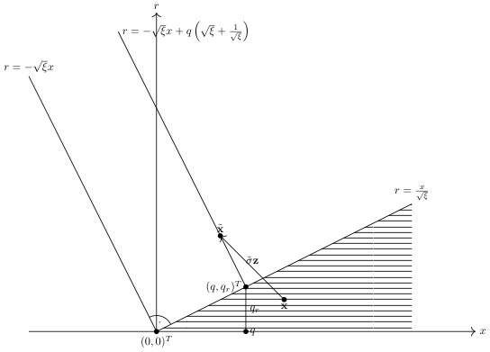 Figure 1
 Figure 2
 Figure 2
 Figure 3
 Figure 3
 Figure 3
 Figure 3
 Figure 4
 Figure 4
 Figure 4
 Figure 4
 Figure 4
 Figure 4
 Figure 4
 Figure 4
 Figure 4
 Figure 5
 Figure 5
 Figure 5
 Figure 5
 Figure 5
 Figure 5
 Figure 5
 Figure 5
 Figure 5
 Figure 6
 Figure 6
 Figure 6
 Figure 6
 Figure 6
 Figure 6
 Figure 7
 Figure 7
 Figure 7
 Figure 7
 Figure 7
 Figure 7
 Figure 8
 Figure 8
 Figure 8
Peer Reviews
No public reviews on file for this paper yet. If you reviewed it on a platform where reviews are public (OpenReview, ICLR, NeurIPS, ICML), you can paste yours below so the community can read it here.
Videos
No videos yet. Explain this paper in a talk, walkthrough, or lecture? Add one.
Analysis of the -CSA-ES
with Repair by Projection Applied to a Conically Constrained Problem
\namePatrick Spettel \[email protected]
\addrResearch Center Process and Product Engineering, Vorarlberg University of Applied Sciences, Dornbirn, 6850, Austria \AND\nameHans-Georg Beyer \[email protected]
\addrDepartment of Computer Science, Research Center Process and Product Engineering, Vorarlberg University of Applied Sciences, Dornbirn, 6850, Austria
Abstract
Theoretical analyses of evolution strategies are indispensable for gaining a deep understanding of their inner workings. For constrained problems, rather simple problems are of interest in the current research. This work presents a theoretical analysis of a multi-recombinative evolution strategy with cumulative step size adaptation applied to a conically constrained linear optimization problem. The state of the strategy is modeled by random variables and a stochastic iterative mapping is introduced. For the analytical treatment, fluctuations are neglected and the mean value iterative system is considered. Non-linear difference equations are derived based on one-generation progress rates. Based on that, expressions for the steady state of the mean value iterative system are derived. By comparison with real algorithm runs, it is shown that for the considered assumptions, the theoretical derivations are able to predict the dynamics and the steady state values of the real runs.
Keywords
Evolution strategy, constraint handling, repair by projection, cumulative step size adaptation, conically constrained problem.
1 Introduction
Thorough theoretical investigations of evolution strategies (ESs) are necessary for gaining a deep understanding of how they work. A lot of research has been done for analyzing ESs applied to unconstrained problems. For the constrained setting, there are still aspects for which a deep theoretical understanding is missing. As a step in that direction, this work theoretically analyzes a -ES with cumulative step size adaptation (CSA) applied to a conically constrained linear problem.
Regarding related work, a -ES with constraint handling by discarding infeasible offspring has been analyzed by Arnold, 2011b for a single linear constraint. Repair by projection has been considered (Arnold, 2011a, ) and a comparison with repair by reflection and repair by truncation has been performed by Hellwig and Arnold, (2016). Based on Lagrangian constraint handling, Arnold and Porter, (2015) presented a -ES applied to a single linear inequality constraint with the sphere model. The one-generation behavior has been analyzed in that work.
A theoretical investigation based on Markov chains for a multi-recombinative variant with Lagrangian constraint handling has been presented by Atamna et al., (2016). Investigation of a single linear constraint in that work has been extended to multiple linear constraints (Atamna et al.,, 2017).
Arnold, (2013) has considered a conically constrained problem. In that work, a -ES is applied to the problem by discarding infeasible offspring. Spettel and Beyer, 2018a have considered the same problem and have analyzed a --Self-Adaptation ES (SA-ES). It has been extended to the multi-recombinative variant (Spettel and Beyer, 2018b, ). The contribution of this paper is the analysis considering CSA instead of SA for the mutation strength control mechanism.
The remainder of the paper is organized as follows. Section 2 introduces the optimization problem under consideration and describes the algorithm that is analyzed. Section 3 concerns the theoretical analysis. First, a mean value iterative system that models the dynamics of the ES is derived in Section 3.1. Second, steady state considerations are shown in Section 3.2. For the theoretical considerations, plots comparing them to results of real ES runs are presented for showing the approximation quality. Finally, Section 4 discusses the results and concludes the paper.
2 Problem and Algorithm
Minimization of
[TABLE]
subject to constraints
[TABLE]
is considered in this work ( and ).
The state of an ES individual can be uniquely described in the -space. It consists of , the distance from [math] in -direction (cone axis), and , the distance from the cone axis. Because isotropic mutations are considered in the ES, the coordinate system can be rotated (w.l.o.g.) such that corresponds to in the parameter space. Figure 1 visualizes the problem. The equation for the cone boundary is , which follows from Equation 2. The projection line can be derived using the cone direction vector and its counterclockwise rotation by 90 degrees yielding . The values and denote a parental individual and an offspring individual, respectively. The corresponding mutation is indicated as . The values of and after projection are denoted by and , respectively.
The algorithm to be analyzed is a -CSA-ES with repair by projection applied to the problem introduced above. Its pseudo code is shown in Algorithm 1. In the beginning, the parameters are initialized (1 to 2). In the generational loop, offspring are created (6 to 16). Each offspring’s parameter vector is sampled from a multivariate normal distribution with mean and standard deviation in 7 and 8. If the generated offspring is infeasible (), its parameter vector is projected onto the point on the boundary of the feasible region that minimizes the Euclidean distance to the offspring point. The corresponding mutation vector leading to this repaired point is calculated back (9 to 12). Projection means solving the optimization problem
[TABLE]
where is the individual to be projected. The function
[TABLE]
is introduced, which returns of the problem (4). Appendix A in the supplementary material of Spettel and Beyer, 2018b shows a geometrical approach for deriving a closed-form solution to the projection optimization problem (4). Given an infeasible individual , it reads
[TABLE]
where . After possible repair, the offspring’s fitness is determined in 13. The next generation’s parental individual (18) and the next generation’s mutation strength (20) are computed next. The next generation’s parental parameter vector is set to the mean of the best (w.r.t. fitness) offspring parameter vectors111Note that the order statistic notation is used to denote the -th best (w.r.t. fitness) out of values. The notation is used to denote the -th element of a vector . It is equivalent to writing .. For the mutation strength update, first the cumulative -vector is updated. The cumulation parameter determines the fading strength. The mutation strength is then updated using this -vector. The parameter acts as a damping factor. If the squared length of the -vector is smaller than , the step size is decreased. Otherwise, the step size is increased. Intuitively, this means that multiple correlated steps allow a larger step size and vice versa. The update of the generation counter ends one iteration of the generation loop. The values , , , , , and are only needed in the theoretical analysis and can be removed in practical applications of the ES. They are indicated in the algorithm in 4, 5, 14, 15, 21 and 22, respectively.
Figure 2 shows an example of the - and -dynamics of Algorithm 1 (solid line) in comparison with results of the closed-form approximate iterative system (dotted line) that is derived in the sections that follow. As one can see, the real dynamics are predicted satisfactorily by the theoretical considerations for the case shown.
3 Theoretical Analysis
To completely describe the state of the ES, the random variables , , and the squared length need to be modeled in addition to the variables for the position in the parameter space, and . The random vector is decomposed into its magnitude along the cone axis and its magnitude in direction of the parental individual’s components
[TABLE]
This leads to a stochastic iterative system of the form
[TABLE]
3.1 Derivation of a Mean Value Iterative System for Modeling the
Dynamics of the ES
Similar to the analysis in Section IV of Spettel and Beyer, 2018b , fluctuation terms are neglected and deterministic evolution equations under asymptotic assumptions are derived. This allows predicting the mean value dynamics of the ES. To make the distinction between the random variable and its mean value in the iterative system clear, is used to denote the expected value of a random variate . Thus, the mean value iterative system is represented as
[TABLE]
This section presents derivations of difference equations for the system (9). In Section 3.1.1, difference equations are presented for expressing with and with by using the respective local progress rates. Section 3.1.2, Section 3.1.3, and Section 3.1.4 deal with the derivation of difference equations for , , and , respectively. They are derived from the corresponding steps of Algorithm 1 and they also make use of the local progress rates. Finally, the difference equation for is stated in Section 3.1.5, the derived system of equations is summarized, and it is compared to real ES runs in Section 3.1.6.
3.1.1 Derivation of Mean Value Difference Equations for
and
The starting points for the derivation of mean value difference equations for and are the progress rates in and direction. Their definitions read
[TABLE]
[TABLE]
They describe the one-generation expected change in the parameter space. The normalizations
[TABLE]
[TABLE]
and
[TABLE]
are introduced in order to have quantities that are independent of the position in the search space. Using Equation 10 with Equation 12 and Equation 11 with Equation 13, the equations
[TABLE]
follow. Approximations for and have already been derived by Spettel and Beyer, 2018b (, Equations (37) and (38)). In that work, expressions for and have been derived under the asymptotic assumptions of sufficiently large values of and . In those derivations, two cases have been distinguished. If one considers the ES being far from the cone boundary, offspring are feasible with overwhelming probability. The opposite case of being in the vicinity of the cone boundary results in infeasible offspring almost surely. These observations allow simplifications for the former case because the projection can be ignored. Both cases are combined into single equations by weighting the feasible and infeasible cases with an approximation for the offspring feasibility and offspring infeasibility probability, respectively. The -distribution in those derivations has been approximated by a normal distribution where
[TABLE]
and
[TABLE]
(it is referred to Appendix B in the supplementary material of Spettel and Beyer, 2018b for the detailed derivation). The results that build the basis for the following CSA analysis are briefly recapped here.222In the further considerations, the symbols “” and “” are used. Expressions in the form of denote that is asymptotically equal to for given asymptotical assumptions (e.g. ). The particular assumptions are stated explicitly for every use of “”. That is, in the limit case of the given assumptions, is equal to . The form is used for cases where is an approximation for with given assumptions that are not of asymptotical nature. In this sense, “” is weaker than “”. The expression for has been derived as
[TABLE]
and the one for reads
[TABLE]
The approximate offspring feasibility probability writes
[TABLE]
where denotes the cumulative distribution function of the standard normal distribution. denotes the infeasible part of Equation 19. The constant is a so-called progress coefficient. A definition is given in (Beyer,, 2001, Eq. 6.102, p. 247). It reads
[TABLE]
3.1.2 Derivation of a Mean Value Difference Equation for
For , a mean value difference equation can be derived using the update rule from 19 of Algorithm 1. Computation of the expected value with directly yields
[TABLE]
can be expressed with the progress rate in -direction . From the definition of the progress rate,
[TABLE]
follows. Therefore,
[TABLE]
holds. Using Equation 27 and Equation 14,
[TABLE]
follows.
3.1.3 Derivation of a Mean Value Difference Equation for
For , a mean value difference equation can be derived using the update rule from 19 of Algorithm 1 and considering Equation 7. To begin with,
[TABLE]
can be derived. Equation 35 can further be rewritten by the introduction of (similar to Equation 7) and use of Equation 14 resulting in
[TABLE]
For the fraction , has to be derived. From the offspring generation and selection steps it follows that
[TABLE]
holds. Using the result from Equation 41,
[TABLE]
can be derived. For further simplification of Equation 42, asymptotic assumptions are made for . Because the mutation vector is corrected in case of projection (11 in Algorithm 1), denotes the centroid of the best (w.r.t. fitness) offspring mutation vectors after the projection step. Approximation of for the asymptotic case by its value before projection and selection yields a normal distribution for , which follows by the properties of a sum of normal distributed random variables.
Hence, can be approximated by a distribution with degrees of freedom. As the expected value of the distribution corresponds to its number of degrees of freedom,
[TABLE]
follows for by the law of large numbers. With Equation 43 and the assumptions and ,
[TABLE]
follows. Making use of Equation 44 and Equation 43, Equation 38 can be simplified for the asymptotic case yielding
[TABLE]
Taking expected values of Equation 47 with results in
[TABLE]
To treat Equation 50 further, and need to be derived.
For , is decomposed into a vector in direction of the parental individual’s components and in a direction that is orthogonal to , i.e., . Further, in the following the assumption is made that those direction vectors are unit vectors, i.e., and . Therefore, can be written as
[TABLE]
where and are the projections of the mutation vector in direction of and , respectively. Using Equation 51,
[TABLE]
follows. Note that corresponds to the definition in Equation 7. Taking into account the statistical independence of the cumulated path vector and the mutation in the current generation, taking expectation results in
[TABLE]
Note that vanishes because the mutations in direction are isotropic and selectively neutral. Hence, the second summand of Equation 53 is [math] in expectation. To investigate the behavior of , the dynamics of have been empirically determined for different parameter configurations in real ES runs (not shown here). It turned out that fluctuates around [math] (with the empirical mean being approximately [math]), which further justifies the step from Equation 53 to Equation 54.
can be calculated from the progress rate of the quadratic distance from the cone axis. It writes
[TABLE]
where denotes the distance from the cone boundary of the centroid after projection (cf. 22 of Algorithm 1). Expressions for and have already been derived in Appendix D in the supplementary material of Spettel and Beyer, 2018b . The used Taylor approximation in Equation (D.157) of that work allows using the square of Equation (D.165) for the feasible case yielding
[TABLE]
Similarly, the Taylor expansion used in Equation (D.172) of that work allows using the square of Equation (D.217) as an approximation for the infeasible case. It reads
[TABLE]
Using Equation 57 and Equation 58,
[TABLE]
follows, where a closed-form approximation
[TABLE]
has been derived in Spettel and Beyer, 2018b as well (refer to the derivations leading to Equation (C.149) in Appendix C in the supplementary of that work for the details). With Equation 59 and Equation 60, can be computed for a given state of the system. The goal is now to express in terms of . Subsequently solving for allows then to compute its value. Using Equation 55 and Equation 41 with Equation 43, can alternatively be written as
[TABLE]
Equation 62 can be solved for yielding
[TABLE]
Reinsertion of Equation 54 and Equation 63 into Equation 50 yields
[TABLE]
3.1.4 Derivation of a Mean Value Difference
Equation for
Using the update rule from 19 of Algorithm 1,
[TABLE]
can be derived. For treating , the vector can be decomposed into a sum of vectors in direction of the cone axis , in direction of the parental individual’s components , and in a direction that is orthogonal to and . Formally, this can be written as
[TABLE]
where and . , , and denote the corresponding projections in those directions. Consequently,
[TABLE]
and subsequently
[TABLE]
follow. Taking into account the statistical independence between the cumulation path and a particular generation’s mutations allows writing
[TABLE]
Again, vanishes because those mutations are selectively neutral and isotropic. Taking expectation of Equation 72, considering Equations 77, 27, 63 and 14, and using ,
[TABLE]
follows.
3.1.5 Derivation of a Mean Value Difference
Equation for
From the update rule of in 20 of Algorithm 1, follows for the update of the mutation strength. Taking expected values and knowing that is constant w.r.t. , this writes . Assuming that the fluctuations of around its expected value are sufficiently small, the expected value can be pulled into the exponential function yielding
[TABLE]
3.1.6 Summary of the Mean Value Difference Equations
[TABLE]
The mean value dynamics of the -CSA-ES on the conically constrained problem are shown in Figure 3 for , , , and . The agreement of the simulations and the derived expressions is satisfactory. In particular, one observes that the lines of the iteration with one-generation experiments are very similar to the lines generated by real ES runs. Consequently, the modeling of the system with Equations 86 to 100 is appropriate and the deviations for the theoretically derived expressions are mainly due to approximations in the derivations of the local progress rates. For this, it is referred to the additional figures provided in the supplementary material (Appendix A). They show a larger deviation for smaller values of and smaller values of . But notice that in those figures the iteration with one-generation experiments for the local progress measures coincides well with the results of real ES runs. This again shows the appropriateness of the modeling in Equations 86 to 100. The deviations for small stem from asymptotic assumptions using . They help simplifying expressions resulting in a theoretical analysis that is tractable. The deviations for small are due to approximations in the derivation of the offspring cumulative distribution function after the projection step in -direction (for the details, it is referred to Section 3.1.2.1.2.3 in Spettel and Beyer, 2018c , in particular to the step from Equation (3.73) to Equation (3.74)).
For the figures, results of real runs of the ES have been averaged for generating the solid lines. The lines for the iteration by approximation have been computed by iterating the mean value iterative system (Equations 86 to 100) with Equations 19, 22 and 59 for (and ), (and ), and , respectively. The lines for the iteration with one-generation experiments have been generated by iterating the system (Equations 86 to 100) and simulating (and ), (and ), and . It can happen that in a generation of iterating the system (Equations 86 to 100), infeasible are created. In such circumstances, the corresponding have been projected back.
3.2 Behavior of the ES in the Steady State
The goal of this section is to derive approximate closed-form expressions for the steady state values of the mean value iterative system that is summarized in Section 3.1.6. A working ES should steadily decrease and (Equation 86 and Equation 88, respectively) in order to move towards the optimizer. For determining the steady state normalized mutation strength value, the fixed point of the system of non-linear equations (Equations 90 to 100) is to be computed.
3.2.1 Derivations Towards Closed-Form Steady State Expressions
This section comprises a first step towards closed-form approximations for the steady state values of the system summarized in Section 3.1.6. Expressions are derived that finally lead to a steady state equation for the normalized mutation strength. A closed form solution of this equation is not apparent. Hence, further assumptions for different cases are considered in the following sections.
To compute the fixed point of the system described by Equations 90 to 100, stationary state expressions , , , and for , , , and , respectively, need to be derived first because they are dependent on the position in the parameter space. The bottom left subplot of Figure 3 shows that the ES moves in the vicinity of the cone boundary in the steady state. This can be seen because the dynamics of and are plotted by converting them into each other for the cone boundary case. Notice that those lines coincide in the steady state. In this situation, for . This follows from Equation 23. By the cone boundary equation (Equation 2), a parental individual is on the cone boundary for . Using this together with Equation 14 and Equation 23 yields
[TABLE]
By taking into account Equation 17,
[TABLE]
follows. If is sufficiently large, .
For the distance ratio , one observes that it approaches a stationary state value . This can be expressed with the condition for sufficiently large values of . Making use of the progress rates (Equations 10 to 13), follows, which implies
[TABLE]
The normalized mutation strength should be constant on average in the steady state for a continuous decrease towards the optimizer. That is, the definition of the steady state normalized mutation strength reads . Expressed as a condition, it can be stated as .
Considering the case of , use of the infeasible case approximations (the infeasible part of Equation 19 and the infeasible part Equation 22) for handling Equation 103, results in
[TABLE]
This can subsequently be rewritten to
[TABLE]
For , the infeasible case approximations can be used. Insertion of Equation 107 into the infeasible part of Equation 19 assuming the expected steady state together with Equation 103 and yields
[TABLE]
for has been used from Equation 111 to Equation 113. In addition, a Taylor expansion with cut-off after the linear term has been applied to .
A steady state expression for is derived next. With Equation 12 and Equation 115,
[TABLE]
can be derived. Use of Equation 107 for the fraction results in
[TABLE]
Similarly, a steady state expression for can be derived. Considering the infeasible case (because in the steady state ) of Equation 59, we have
[TABLE]
According to 21 and 4 of Algorithm 1, . Hence, Equation 118 can be rewritten using Equation 15 for the infeasible case and Equation 107 for , resulting in
[TABLE]
Using Equation 117 and Equation 119, steady state expressions for Equations 90 to 100 can be derived. Requiring in Equation 90 using Equation 117 yields
[TABLE]
Analogously, requiring in Equation 93 using Equation 119 results in
[TABLE]
In the same way, setting in Equation 96 using Equation 117 and Equation 119 gives
[TABLE]
For the mutation strength,
[TABLE]
follows from 20 of Algorithm 1 with the use of Equation 14. Rewriting Equation 123 and using Equation 42 together with Equation 43 for the fraction , we have
[TABLE]
Use of the Taylor expansion (around zero and neglecting terms of quadratic and higher order) results in
[TABLE]
Computing the expectation of Equation 126 and requiring , we get
[TABLE]
Usage of Equation 63 together with the steady state expression derived in Equation 119 for results in
[TABLE]
Consideration of Equations 115, 120, 121 and 122 allows numerically solving Equation 129 for .
3.2.2 Derivation of Closed-Form Approximations for the Steady State
with the Assumptions and
The goal of this section is to simplify the expressions derived in Section 3.2.1 further using additional asymptotic assumptions in order to arrive at closed-form steady state approximations.
The expression derived for as Equation 119 is simplified further yielding
[TABLE]
In Equation 131, has been assumed and therefore the second summand has been neglected.
Insertion of Equation 131 into Equation 129 replacing yields (after simplification)
[TABLE]
for the steady state mutation strength equation. Equation 131 can also be inserted into Equation 121 replacing . This results in
[TABLE]
With the assumptions and , the expression is an order of magnitude smaller than c and can therefore be neglected w.r.t. c. Hence, Equation 134 simplifies to
[TABLE]
Similarly, Equation 131 inserted into Equation 122 replacing results in
[TABLE]
Insertion of Equation 135 and Equation 120 into Equation 136 yields (after straight-forward simplification)
[TABLE]
for allows writing
[TABLE]
From Equation 138 to Equation 139, has been substituted by Equation 115, its square has been calculated, and the resulting expression has been simplified.
With this, insertion of Equation 115 and Equation 139 into Equation 132 yields the quadratic equation
[TABLE]
for the steady state normalized mutation strength equation. By solving Equation 140 for the positive root (because ) with subsequent simplification of the result we get
[TABLE]
as an asymptotic () closed-form expression for the steady state normalized mutation strength. Insertion of and into Equation 141 results in the expression
[TABLE]
Assuming and allows a further asymptotic simplification of Equation 142 (neglecting , , , , and ) resulting in
[TABLE]
For sufficiently large , , and Equation 143 writes . Back-insertion of Equation 141 (or Equation 143) into Equations 107, 115, 120, 121 and 122 allows calculating the steady state distance from the cone boundary, the normalized steady state progress, , , and .
Figure 4 shows plots of the steady state computations. Results computed by Equation 141 have been compared to real ES runs. The values for the points denoting the approximations have been determined by computing the normalized steady state mutation strength using Equation 141 for different values of . The results for and have been determined by using the computed steady state values with Equation 115. The approximations for have been determined by evaluating Equation 107. The values for the points denoting the experiments have been determined by computing the averages of the particular values in real ES runs. The figures show that the derived expressions get better for larger values of and . Again, the deviations for small are due to approximations in the derivation of the local progress rates. The deviations for small stem from the use of asymptotic assumptions .
3.2.3 Derivation of Closed-Form Approximations for the Steady State
with the Assumptions and
In Section 3.2.2 it has been assumed that from Equation 134 to Equation 135. This section presents a derivation for the case . To this end, Equation 133 is rewritten to
[TABLE]
With , we have . This together with the assumption allows rewriting Equation 144 to
[TABLE]
With the additional assumption , Equation 145 simplifies to
[TABLE]
Insertion of Equation 146 and Equation 120 into Equation 136 yields
[TABLE]
In the step from Equation 147 to Equation 148, for has been used.
Insertion of Equation 115 and Equation 148 into Equation 132 yields
[TABLE]
for the steady state mutation strength equation. By assuming , Equation 149 simplifies. Together with grouping the powers of it writes
[TABLE]
Introducing common denominators allows rewriting Equation 150 to
[TABLE]
Simplification of Equation 151 using and results in
[TABLE]
Note that multiplying Equation 152 by results in a cubic equation that can be solved. However, the expressions for the closed-form solutions are rather long. Hence, a quadratic equation is aimed for. To this end, Equation 152 is approximated quadratically. Neglecting and in Equation 152 results in333Plots of further approximations are presented in the supplementary material (Appendix B).
[TABLE]
Solving Equation 153 for the positive root with subsequent simplification yields
[TABLE]
Figure 5 shows plots of the steady state computations. Results computed by Equation 154 have been compared to real ES runs. The values for the points denoting the approximations have been determined by computing the normalized steady state mutation strength using Equation 154 for different values of . The results for and have been determined by using the computed steady state values with Equation 115. The approximations for have been determined by evaluating Equation 107. The values for the points denoting the experiments have been determined by computing the averages of the particular values in real ES runs.
4 Conclusions
In this work, the -CSA-ES has been theoretically analyzed. For this, a mean value iterative system has been introduced and compared to real ES runs. Based on this derived system, steady state expressions have been derived and compared to ES simulations.
The comparison of the mean value iterative system summarized in Section 3.1.6 with real ES runs shows a satisfactory agreement of the theory and simulations for large and large (see Figure 3). The deviations for small are due to the asymptotic assumptions that are used in the derivations of the microscopic and macroscopic aspects of the ES. They are used to simplify the expressions and thus make a theoretical analysis tractable. The deviations for small stem from the derivation of the offspring cumulative distribution function after the projection step in -direction (for the details, it is referred to Section 3.1.2.1.2.3 in Spettel and Beyer, 2018c , in particular to the step from Equation (3.73) to Equation (3.74)). The same observations regarding the deviations can be made for the derived steady state expressions (see Figures 4 and 5).
For the steady state derivations, it is of particular interest to compare the results obtained in this work for the CSA-ES with the results obtained for the SA-ES. The -SA-ES has been theoretically analyzed by Spettel and Beyer, 2018b applied to the same conically constrained problem. In that work, the microscopic and macroscopic aspects of the -SA-ES have been investigated. For the microscopic aspects, expressions for the local progress for and and the self-adaptation response (SAR) function have been derived using asymptotic assumptions. Those results have then been used for the macroscopic analysis. The mean value dynamics generated by iteration using those local measures have been compared to real runs. In addition, steady state expressions have been derived and discussed. They show that the SA-ES is able to achieve sufficiently high mutation strengths to keep the progress almost constant for increasing . Surprisingly, for the CSA-ES, the choice of the cumulation parameter has a qualitative influence on the behavior.
Considering the choice of proposed in early publications on CMA-ES (Hansen and Ostermeier,, 1997), the steady state mutation strengths attained flatten with increasing . As a consequence, the steady state progress decreases with higher values of . This can be seen by considering Equation 143 that leads to for sufficiently large . For and , this results in a steady state normalized mutation strength of approximately . Note that this value corresponds to the approximations for the larger values of shown in Figure 4 (right-most column, ). Equation 143 can be inserted into the steady state progress rate (Equation 115) yielding
[TABLE]
From the simplified result of Equation 155 one immediately notices that for (respecting that was used in the derivations leading to Equation 143). This is exactly what one sees in Figure 4, the stationary state progress decreases with increasing .
In contrast, for the case that is proposed in newer publications ( by Hansen and Ostermeier, (2001) or by Hansen, (2016), both of which are in for ), the steady state mutation strength increases with increasing . It is therefore able to achieve a constant progress rate for increasing . The steady state progress is less than that of the SA-ES. Due to the increase of with increasing , the increasing deviations of the approximation from the simulations can be explained. In the derivations leading to Equation 44, it has been assumed that . As the steady state increases with , must be increased in order to have the same approximation quality for higher values of . This can be explained more formally. Assuming large , holds in Equation 154. Hence,
[TABLE]
follows, which - for large - is of the same order as the one of the SA-ES (see Eq. (62) in Spettel and Beyer, 2018b ). While it is common practice to use since the seminal CMA-ES paper (Hansen and Ostermeier,, 2001), this is the first theoretical result that shows an advantage of the choice.
A further aspect for discussion is the special case of the non-recombinative -CSA-ES that is contained in the derivations for the -CSA-ES. The iterative system for the non-recombinative () case can be derived analogously to the multi-recombinative () case. The resulting equations differ in the expressions for , , and . It has been investigated further (not shown here) and for the mean value iterative systems of the -CSA-ES and the -CSA-ES agree. An interesting observation between the case and the case is the evolution near the cone boundary. Whereas the CSA-ES with evolves on the boundary, the CSA-ES with attains a certain steady state distance from the boundary (cf. the bottom subfigures of Figure 4 and Figure 5). Considering a parental individual on the cone boundary, the offspring are infeasible with overwhelming probability for sufficiently large . Hence, they are repaired by projection and are on the boundary after projection. In particular, the best of them is on the boundary. Therefore, for , the ES evolves on the boundary. For , the centroid computation after projection results in offspring that are inside the feasible region.
To conclude the paper, topics for future work are outlined. In addition to the SA and the CSA for the control mechanism, it is of interest to investigate the behavior of Meta-ESs applied to the conically constrained problem. Comparison of the repair by projection approach with other repair methods is another topic for further research. Analysis of ESs applied to other constrained problems is another research direction for the future.
Acknowledgments
This work was supported by the Austrian Science Fund FWF under grant P29651-N32.
Appendix A Additional Results Comparing the Derived Approximations with
Simulations
Figures 6 to 11 show the mean value dynamics of the -CSA-ES applied to the conically constrained problem with different parameters as indicated in the title of the subplots. The plots are organized into three rows and two columns. The first two rows show the (first row, first column), (first row, second column), (second row, first column), and (second row, second column) dynamics. The third row shows and converted into each other by . The third row shows that after some initial phase, the ES transitions into a stationary state. In this steady state, the ES moves along the cone boundary. This becomes clear in the plots because the equation for the cone boundary is or equivalently . In the first two rows, the solid line has been generated by averaging real runs of the ES. The dashed line has been determined by iterating the mean value iterative system of Section 3.1.6 with one-generation experiments for , , , , and . The dotted lines have been computed by iterating the mean value iterative system with the derived approximations as indicated in the derivations leading to the equations in Section 3.1.6 for , , , , and . Due to the approximations used it is possible that in a generation , the iteration of the mean value iterative system yields infeasible . In such cases, the particular have been projected back and projected values have been used in the further iterations.
Appendix B Further Investigations Considering the Derivation of Closed-Form
Approximations for the Steady State with the Assumptions and
By plotting the left-hand side of (152) for different parameters, one observes that for the values of interest (), the function is quadratic.
Inspired by that, a Taylor expansion around is performed up to and including the quadratic term. It results in a quadratic equation that can be solved for . Figure 12 shows plots of the steady state computations with this approximation compared to real ES runs. The values for the points denoting the approximations have been determined by computing the normalized steady state mutation strength using the solution of the mentioned quadratic equation that has been derived by a Taylor expansion. The results for and have been determined by using the computed steady state values with Equation 115. The approximations for have been determined by evaluating Equation 107. The values for the points denoting the experiments have been determined by computing the averages of the particular values in real ES runs.
Neglecting terms already in Equation 152 is another approach to arrive at a simpler approximate form. Neglecting in Equation 152, results in
[TABLE]
Solving Equation B.1 for the positive root yields
[TABLE]
Figure 13 shows plots of the steady state computations. Results computed by Equation B.2 have been compared to real ES runs. The values for the points denoting the approximations have been determined by computing the normalized steady state mutation strength using Equation B.2 for different values of . The results for and have been determined by using the computed steady state values with Equation 115. The approximations for have been determined by evaluating Equation 107. The values for the points denoting the experiments have been determined by computing the averages of the particular values in real ES runs.
The reference list from the paper itself. Each links out to its DOI / PubMed record.
- 1(1) Arnold, D. V. (2011 a). Analysis of a repair mechanism for the (1, λ 𝜆 \lambda )-ES applied to a simple constrained problem. In Proceedings of the 13th Annual Conference on Genetic and Evolutionary Computation , pages 853–860. ACM.
- 2(2) Arnold, D. V. (2011 b). On the behaviour of the (1, λ 𝜆 \lambda )-ES for a simple constrained problem. In Proceedings of the 11th Workshop Proceedings on Foundations of Genetic Algorithms , pages 15–24. ACM.
- 3Arnold, (2013) Arnold, D. V. (2013). On the behaviour of the (1, λ 𝜆 \lambda )-ES for a conically constrained problem. In Proceedings of the 15th Annual Conference on Genetic and Evolutionary Computation , pages 423–430. ACM.
- 4Arnold and Porter, (2015) Arnold, D. V. and Porter, J. (2015). Towards an augmented Lagrangian constraint handling approach for the (1+1)-ES. In Proceedings of the 2015 Annual Conference on Genetic and Evolutionary Computation , GECCO ’15, pages 249–256, New York, NY, USA. ACM.
- 5Atamna et al., (2016) Atamna, A., Auger, A., and Hansen, N. (2016). Augmented Lagrangian constraint handling for CMA-ES - case of a single linear constraint. In International Conference on Parallel Problem Solving from Nature , pages 181–191. Springer.
- 6Atamna et al., (2017) Atamna, A., Auger, A., and Hansen, N. (2017). Linearly convergent evolution strategies via augmented Lagrangian constraint handling. In Proceedings of the 14th ACM/SIGEVO Conference on Foundations of Genetic Algorithms , pages 149–161. ACM.
- 7Beyer, (2001) Beyer, H.-G. (2001). The Theory of Evolution Strategies . Natural Computing Series. Springer.
- 8Hansen, (2016) Hansen, N. (2016). The CMA evolution strategy: A tutorial. ar Xiv:1604.00772 [cs.LG]. Available online: http://arxiv.org/abs/1604.00772 (accessed Jun 07, 2017).