Solar wind charge exchange in cometary atmospheres. II. Analytical model
Cyril Simon Wedlund, E. Behar, E. Kallio, H. Nilsson, M. Alho, H., Gunell, D. Bodewits, A. Beth, G. Gronoff, R. Hoekstra

TL;DR
This paper develops an analytical model for solar wind charge exchange processes at comets, providing insights into ion distributions, neutral atom production, and solar wind interactions, validated with data from the Rosetta mission to comet 67P.
Contribution
It introduces a comprehensive analytical formalism for charge-changing reactions at comets, including effects of double charge exchange and solar wind parameters, enhancing understanding of cometary atmospheres.
Findings
Double charge exchange significantly affects helium neutral atom production below 200 km/s solar wind speed.
Model predicts a sharp decrease in solar wind ion fluxes near perihelion, forming a solar wind ion cavity.
Retrieval methods for outgassing rates and upstream solar wind fluxes from in situ measurements are discussed.
Abstract
Solar wind charge-changing reactions are of paramount importance to the physico-chemistry of the atmosphere of a comet because they mass-load the solar wind through an effective conversion of fast, light solar wind ions into slow, heavy cometary ions. The ESA/Rosetta mission to comet 67P/Churyumov-Gerasimenko (67P) provided a unique opportunity to study charge-changing processes in situ. An extended analytical formalism describing solar wind charge-changing processes at comets along solar wind streamlines is presented. It is based on a thorough book-keeping of available charge-changing cross sections of hydrogen and helium particles in a water gas. After presenting a general 1D solution of charge exchange at comets, we study the theoretical dependence of charge-state distributions of (He, He, He) and (H, H, H) on solar wind parameters at comet 67P. We show…
Click any figure to enlarge with its caption.
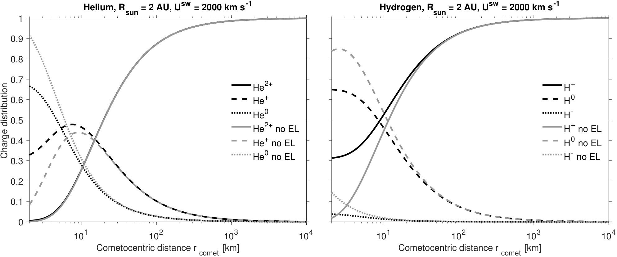 Figure 1
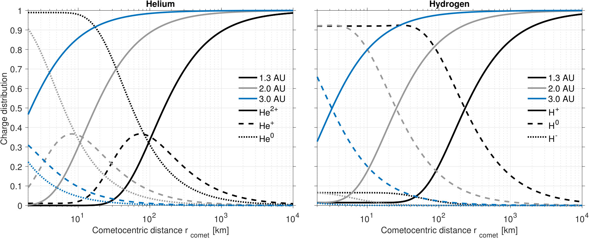 Figure 2
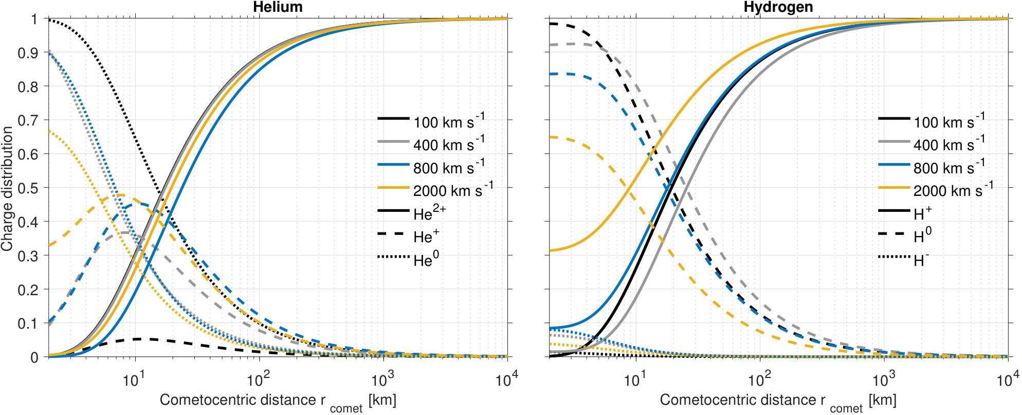 Figure 3
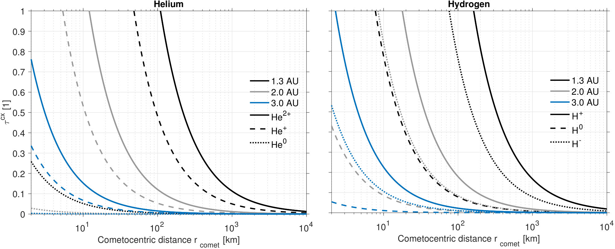 Figure 4
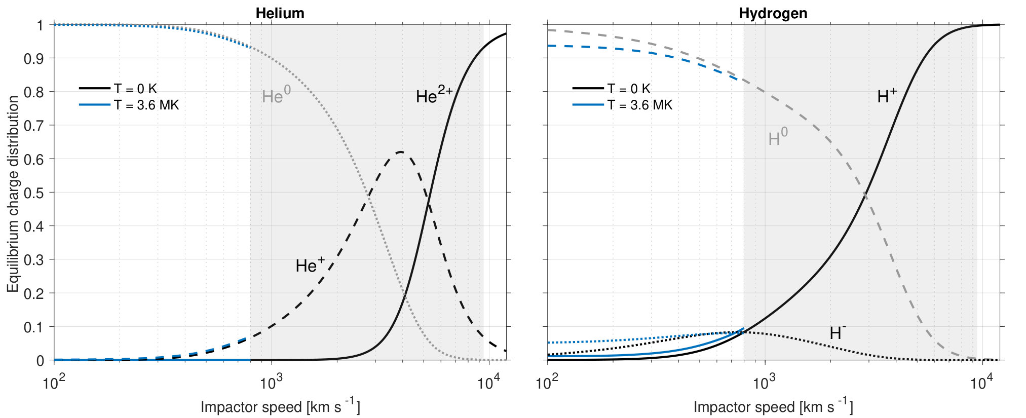 Figure 5
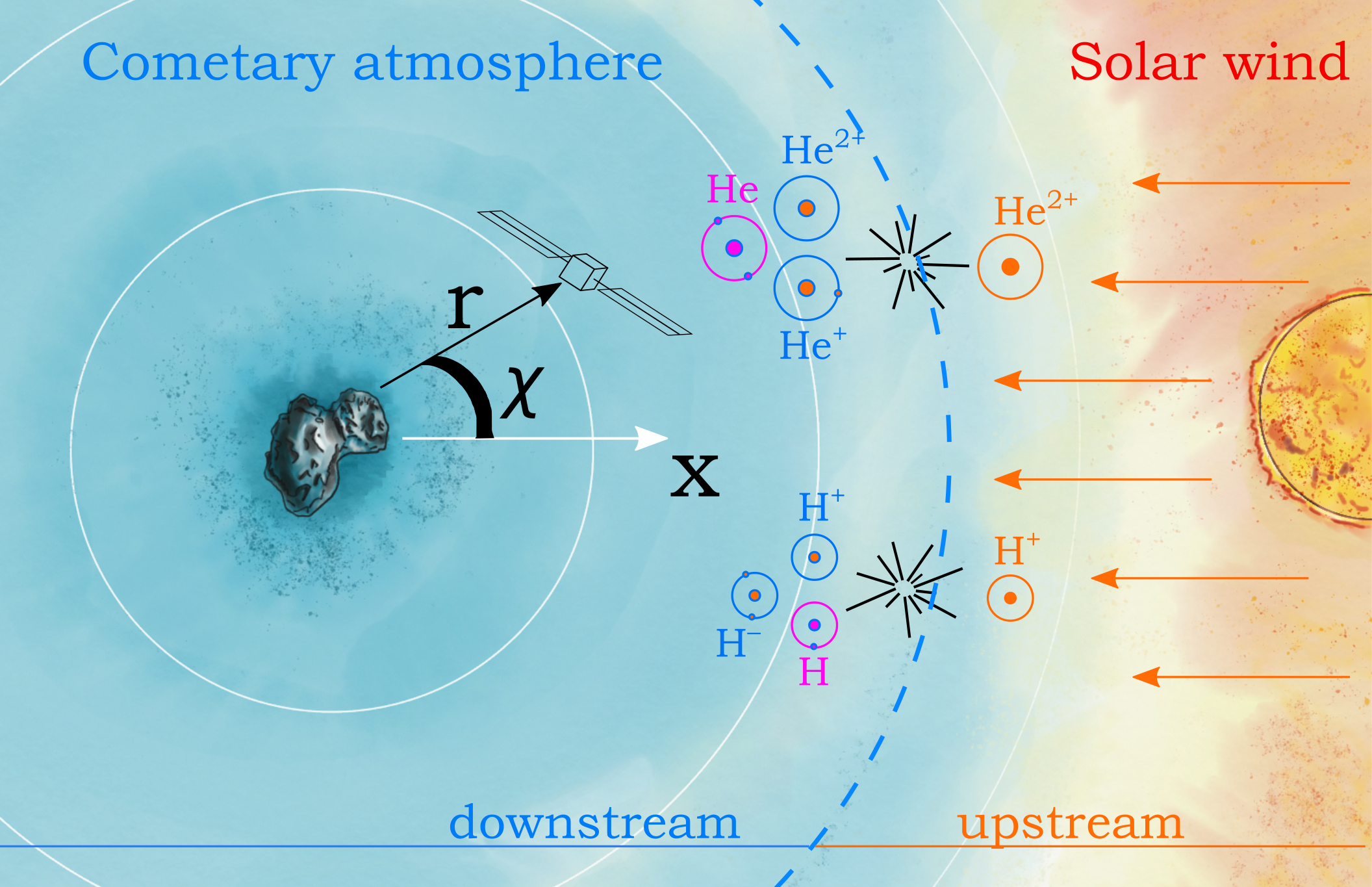 Figure 6
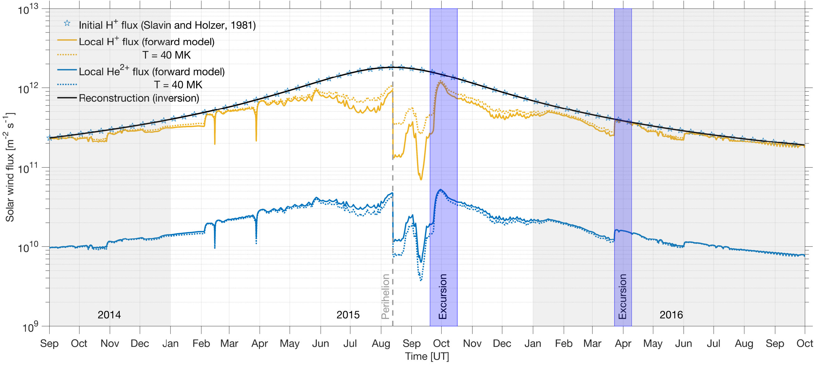 Figure 7
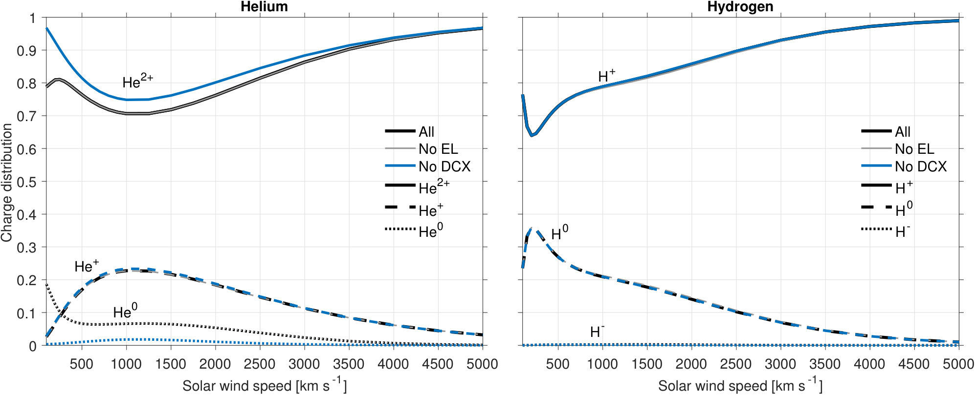 Figure 8
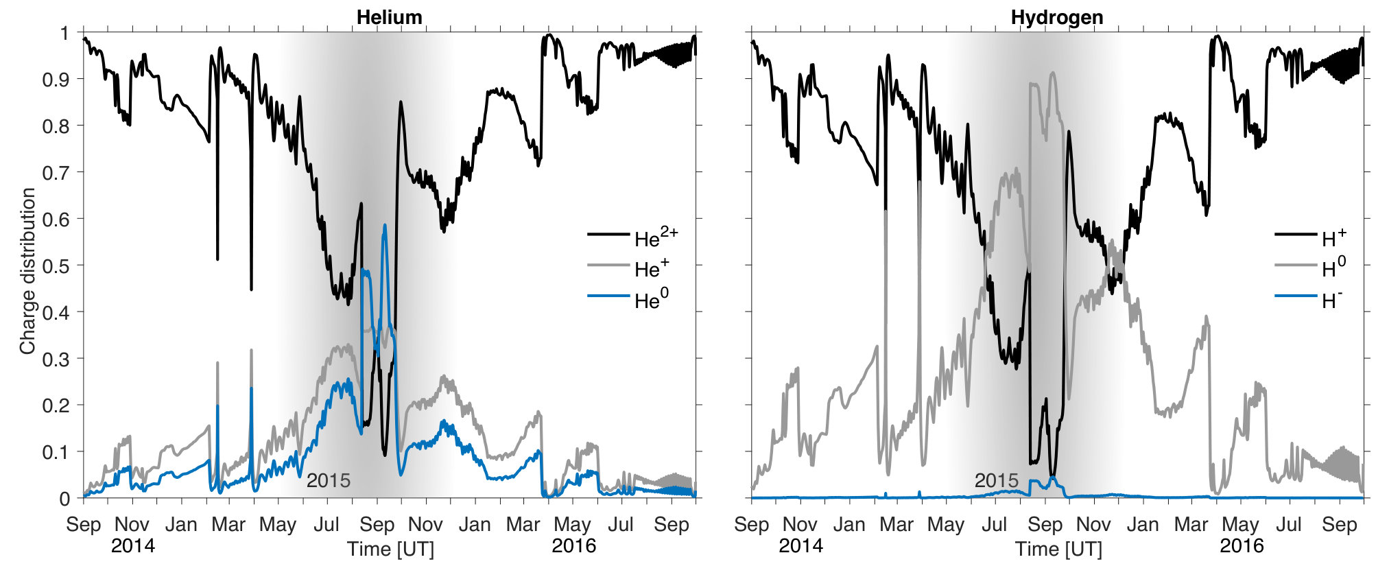 Figure 9
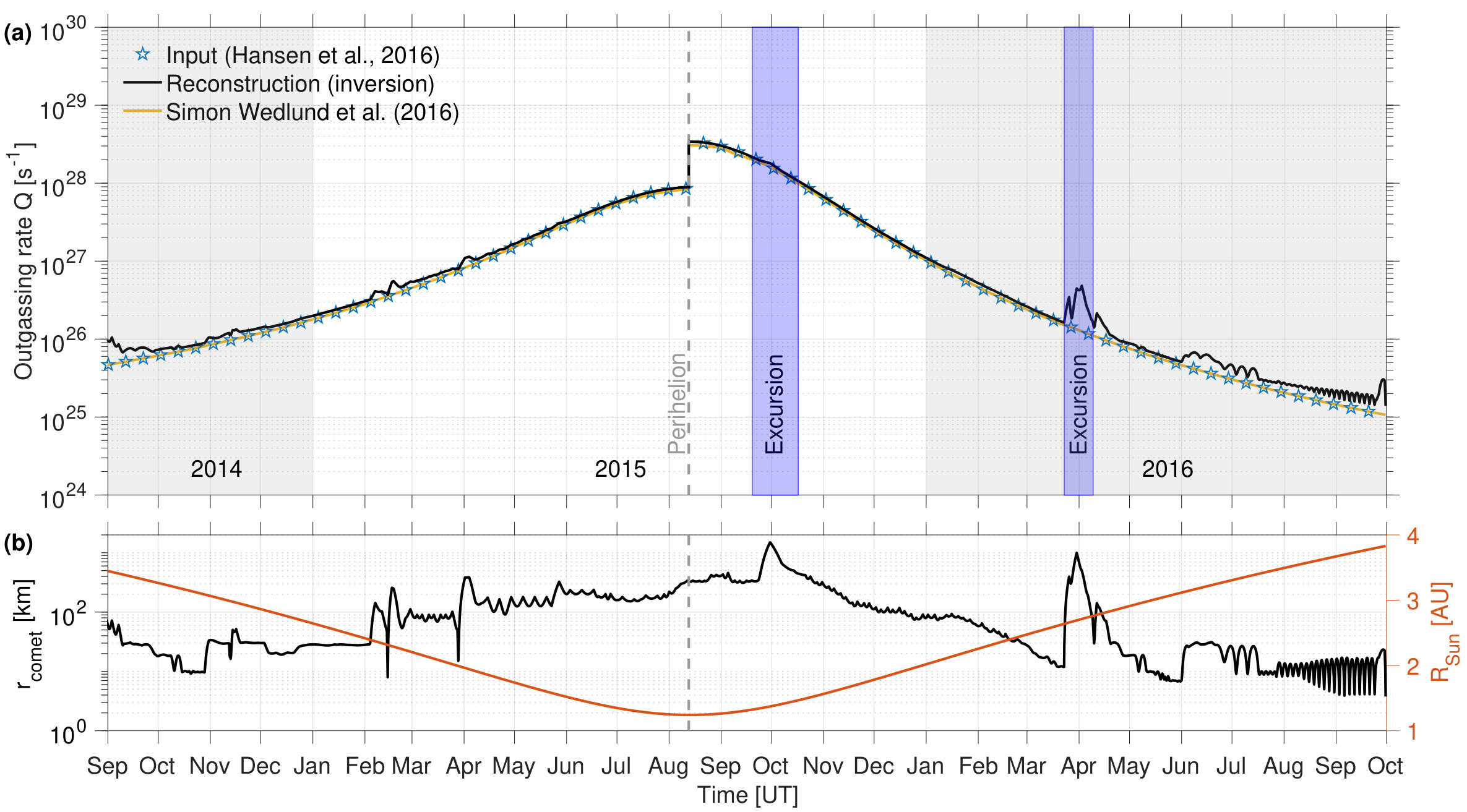 Figure 10
Peer Reviews
No public reviews on file for this paper yet. If you reviewed it on a platform where reviews are public (OpenReview, ICLR, NeurIPS, ICML), you can paste yours below so the community can read it here.
Videos
No videos yet. Explain this paper in a talk, walkthrough, or lecture? Add one.
11institutetext: Department of Physics, University of Oslo, P.O. Box 1048 Blindern, N-0316 Oslo, Norway
11email: [email protected] 22institutetext: Swedish Institute of Space Physics, P.O. Box 812, SE-981 28 Kiruna, Sweden 33institutetext: Luleå University of Technology, Department of Computer Science, Electrical and Space Engineering, Kiruna, SE-981 28, Sweden 44institutetext: Department of Electronics and Nanoengineering, School of Electrical Engineering, Aalto University, P.O. Box 15500, 00076 Aalto, Finland 55institutetext: Royal Belgian Institute for Space Aeronomy, Avenue Circulaire 3, B-1180 Brussels, Belgium 66institutetext: Department of Physics, Umeå University, 901 87 Umeå, Sweden 77institutetext: Physics Department, Auburn University, Auburn, AL 36849, USA 88institutetext: Department of Physics, Imperial College London, Prince Consort Road, London SW7 2AZ, United Kingdom 99institutetext: Science directorate, Chemistry & Dynamics branch, NASA Langley Research Center, Hampton, VA 23666 Virginia, USA 1010institutetext: SSAI, Hampton, VA 23666 Virginia, USA 1111institutetext: Zernike Institute for Advanced Materials, University of Groningen, Nijenborgh 4, 9747 AG, Groningen, The Netherlands
Solar wind charge exchange in cometary atmospheres
II. Analytical model
Cyril Simon Wedlund 11
Etienne Behar 2233
Esa Kallio 44
Hans Nilsson 2233
Markku Alho 44
Herbert Gunell 5566
Dennis Bodewits 77
Arnaud Beth 88
Guillaume Gronoff 991010
Ronnie Hoekstra 1111
Abstract
*Context. *Solar wind charge-changing reactions are of paramount importance to the physico-chemistry of the atmosphere of a comet because they mass-load the solar wind through an effective conversion of fast, light solar wind ions into slow, heavy cometary ions. The ESA/Rosetta mission to comet 67P/Churyumov-Gerasimenko (67P) provided a unique opportunity to study charge-changing processes in situ.
*Aims. *To understand the role of charge-changing reactions in the evolution of the solar wind plasma and to interpret the complex in situ measurements made by Rosetta, numerical or analytical models are necessary.
*Methods. *An extended analytical formalism describing solar wind charge-changing processes at comets along solar wind streamlines is presented. It is based on a thorough book-keeping of available charge-changing cross sections of hydrogen and helium particles in a water gas.
Results. After presenting a general 1D solution of charge exchange at comets, we study the theoretical dependence of charge-state distributions of (He2+, He+, He0) and (H*+, H0, H-) on solar wind parameters at comet 67P. We show that double charge exchange for the HeH2O system plays an important role below a solar wind bulk speed of km s-1* , resulting in the production of He energetic neutral atoms, whereas stripping reactions can in general be neglected. Retrievals of outgassing rates and solar wind upstream fluxes from local Rosetta measurements deep in the coma are discussed. Solar wind ion temperature effects at km s*-1* solar wind speed are well contained during the Rosetta mission.
*Conclusions. *As the comet approaches perihelion, the model predicts a sharp decrease of solar wind ion fluxes by almost one order of magnitude at the location of Rosetta, forming in effect a solar wind ion cavity. This study is the second part of a series of three on solar wind charge-exchange and ionization processes at comets, with a specific application to comet 67P and the Rosetta mission.
Key Words.:
** comets: general – comets: individual: 67P/Churyumov-Gerasimenko – instrumentation: detectors – solar wind, methods: analytical – solar wind: charge-exchange processes – Methods: analytical**
1 Introduction
Over the past decades, evidence of charge-exchange (CX) reactions has been discovered in astrophysics environments, from cometary and planetary atmospheres to the heliosphere and to supernovae environments (Dennerl, 2010). They consist of the transfer of one or several electrons from the outer shells of neutral atoms or molecules, denoted M, to an impinging ion, noted Xi+, where is the initial charge number of species X. Electron capture of electrons takes the form
[TABLE]
From the point of view of the impinging ion, a reverse charge-changing process is the electron loss (or stripping); starting from species , it results in the emission of electrons:
[TABLE]
For , the processes are referred to as one-electron charge-changing reaction; for , two-electron or double charge-changing reactions, and so on. The qualifier ”charge-changing” encompasses both capture and stripping reactions, whereas ”charge exchange” denotes electron capture reactions only. Moreover, ”[M]” refers here to the possibility for compound M to undergo, in the process, dissociation, excitation, and ionization, or a combination of these processes.
Charge exchange was initially studied as a diagnostic for man-made plasmas (Isler, 1977; Hoekstra et al., 1998). The discovery by Lisse et al. (1996) of X-ray emissions at comet Hyakutake C/1996 B2 was attributed by Cravens (1997) to charge-transfer reactions between highly charged solar wind oxygen ions and the cometary neutral atmosphere. Since this first discovery, cometary CX emission has successfully been used to remotely measure the speed of the solar wind (Bodewits et al., 2004a), measure its composition (Kharchenko et al., 2003), and thus the source region of the solar wind (Bodewits et al., 2007; Schwadron & Cravens, 2000), map plasma interaction structures (Wegmann & Dennerl, 2005), and more recently, to determine the bulk composition of cometary atmospheres (Mullen et al., 2017).
Observations of charge-exchanged helium, carbon, and oxygen ions were made during the Giotto mission flyby to comet 1P/Halley and were reported by Fuselier et al. (1991), who used a simplified continuity equation (as in Ip, 1989) to describe CX processes. Bodewits et al. (2004a) reinterpreted their results with a new set of cross sections. More recently, the European Space Agency (ESA) Rosetta mission to comet 67P/Churyumov-Gerasimenko (67P) between August 2014 and September 2016 has provided a unique opportunity for studying CX processes in situ and for an extended period of time (Nilsson et al., 2015a; Simon Wedlund et al., 2016). The observations need to be interpreted with the help of analytical and numerical models.
As the solar wind impinges on a neutral atmosphere, either in expansion (comets) or gravity-bound (planets), charge-transfer collisions effectively result in the replacement of the incoming fast (solar wind) ion by a slow-moving (atmospheric) ion (Dennerl, 2010). Through conservation of energy and momentum, mass loading of the solar wind occurs and is responsible for the deflection and slowing down of the solar wind ions upstream of the cometary nucleus (see Behar et al., 2016a, b, for comet 67P). For comet 67P, which has a relatively low outgassing rate, the atmosphere is essentially a mixture of H2O, CO2 , and CO molecules (Hässig et al., 2015; Fougere et al., 2016). As a first approximation, we only consider capture and stripping collisions in H2O, because this species represents the bulk of the cometary gas during the Rosetta mission, except at large heliocentric distances (above about astronomical units or AU, see Läuter et al., 2019). These reactions result in the production of energetic neutral atoms (ENAs, such as H and He), which continue to travel in straight lines from their production region, and further interact with the ion and neutral environment.
At comet 67P, evidence of solar wind charge transfer is readily seen in the observations of the Rosetta Plasma Consortium (RPC) ion and electron spectrometers. Nilsson et al. (2015a, b) and Simon Wedlund et al. (2016) have reported the detection of He+ ions with the RPC Ion Composition Analyser (RPC-ICA, Nilsson et al., 2007), arising from incoming charge-exchanged He2+ solar wind ions.
Numerical and analytical models have been developed to account for the detected ion fluxes. Khabibrakhmanov & Summers (1997) developed a 1D hydrodynamic model of CX and photoionization at comet 1P/Halley, concluding that the position of the bow shock shifted outward when taking into account single-electron capture of protons in water. Ekenbäck et al. (2008) used a magnetohydrodynamics (MHD) model to produce images of hydrogen ENA emissions around a comet similar to comet 1P/Halley at perihelion. Simon Wedlund et al. (2016) proposed in a recent paper a simple 1D analytical model, using only one electron capture reaction (He He*+*) to account for the He+ fluxes that were routinely measured by RPC-ICA on board Rosetta. The authors showed that from the local measurement of flux ratios in the inner coma, it was possible to infer the total outgassing rate of the comet. Comparison with in situ derived outgassing rates by the Rosetta Orbiter Spectrometer for Ion and Neutral Analysis Comet Pressure Sensor (ROSINA-COPS) (Balsiger et al., 2007) showed that with these simple assumptions, month-to-month differences between the RPC-ICA-inferred and ROSINA-measured water outgassing rates remained within a factor (Hansen et al., 2016). In parallel, using a new quasi-neutral hybrid model of the cometary plasma environment, Simon Wedlund et al. (2017) studied the interplay between ionization processes in the formation of boundaries at comet 67P. They showed that CX plays a major role at large cometocentric distances ( km at a heliocentric distance of AU), whereas photoionization and electron ionization (sometimes referred to as ”electron impact ionization”) is the main source of new cometary ions in the inner coma (Bodewits et al., 2016). This is in agreement with observations of electron densities combined with a more precise ionospheric modeling (Galand et al., 2016; Heritier et al., 2017, 2018).
During the Rosetta mission and while approaching perihelion, the solar wind experienced increasing angular deflection with respect to the Sun-comet line, defining a so-called ”solar wind ion cavity” (Behar et al., 2017, noted SWIC for short). This is due to the increased cometary outgassing activity and mass loading during that period of time, spanning April to December 2015. As a result, and except for a few occasional appearances due to Rosetta excursions at large cometocentric distances, no He2+ and He+ signal could be simultaneously detected in the SWIC (Simon Wedlund et al., 2016; Nilsson et al., 2017b; Behar et al., 2017).
Charge-state distributions and their evolution with respect to outgassing rate and cometocentric distance represent a proxy for the efficiency of charge-changing reactions at a comet such as 67P, as sketched in Fig. 1. In our companion paper (Simon Wedlund et al., 2018b, subsequently referred to as Paper I), we gave recommended charge-changing and ionization cross sections for helium and hydrogen particles colliding with a water gas.
In this study (referred to as Paper II), we expand the initial approach expounded in Simon Wedlund et al. (2016) to include all six main charge-changing cross sections, and present a general analytical solution of the three-component system of helium and hydrogen, with physical implications specific to comets. The forward model expressions are given, and two inversions are proposed, one for deriving the outgassing rate of the comet, one for estimating the upstream solar wind flux from in-situ ion observations. In Section 3, and using our recommended set of cross sections (see Paper I), we explore the dependence of the charge-state distribution at comet 67P on heliocentric and cometocentric distances, and solar wind speed and temperature. From geometrical considerations only, we finally make predictions for the charge-state distribution at comet 67P at the location of Rosetta (Section 3.4).
2 Solar wind charge distributions at a comet
It is well known in the experimental community that charge-state fractions follow a system of coupled differential equations that can be solved analytically: Allison (1958) (and associated erratum Allison, 1959), and later Tawara & Russek (1973), for example, give expressions of the charge-state fractions of helium and hydrogen beams in gases for laboratory diagnostic in the measurement of charge-changing cross sections. In these experiments, beams of incoming ions are set to collide, usually in a vacuum chamber, through solid foils or in gases of known characteristics or neutral densities.
In this section, we apply such a formalism to a cometary environment. We give the equations in matrix form for an -component system of solar wind projectiles, with the number of charge states arising from the charge-changing reactions. We generalize the solution using exponential matrices, and apply this formalism to a three-component charge-changing system between (He2+, He+, He0) and (H*+*, H0, H-) solar wind projectiles and a cometary atmosphere, with . Inversions of the forward solution include the determination from local observations of the neutral outgassing rate of the comet, as well as that of an estimate of the solar wind upstream flux. Matrices and vectors are denoted in bold font. The nomenclature of the explicit solution is loosely inspired by Allison’s, when needed.
In the following, the CX forward model and its inversions are described for the helium system. For completeness, the solution for the hydrogen system is given in Appendix A.
2.1 General model of charge-changing reactions
A solar wind plasma species X of initial charge will undergo electron capture and loss reactions when interacting with cometary neutral species M:
[TABLE]
resulting in one reaction in the capture of electrons by species X and the ionization of neutral compound [M], and in the other, in the loss of electrons by species X. [M] denotes all possible dissociation, excitation, and ionization stages of species M. In doing so, from the plasma point of view, fast, usually light, solar wind ions are depleted in favor of the production of slow-moving heavy cometary ions because the neutral gas has velocities of about km s*-1* (Hansen et al., 2016), which are added to the solar wind flow. This is one of the basic aspects of solar-wind mass loading (Behar et al., 2016b).
2.1.1 Continuity matrix system
In the fluid approximation, the continuity equation for solar wind species Xi+ of density along bulk velocity can be written as
[TABLE]
with and its source and loss terms. To simplify this equation, two assumptions can be made: the upstream solar wind is not time dependent, and so (stationary case), and we assume that all particles of solar wind origin are moving along the solar wind bulk velocity , with abscissa in the Sun-comet direction, with no deviation to their initial direction. Remarking that particle flux , we obtain
[TABLE]
where is the ion temperature of ion species of charge .
Source and loss terms generally depend on the path that the solar wind ions are having as a bulk (following bulk velocity along streamline ), but also on the ion temperature , that is, the path of the individual ion (). We show below that the effect of the temperature of the solar wind ions can be taken into account a posteriori, using for example Maxwellian-averaged cross sections at a given ion temperature (see Paper I), in order to mimic the change in efficiency of the reactions. Here, we subsequently assume for simplicity that all ions of different charge have the same temperature, and that . Moreover, we have implicitly assumed that all charge states follow the same path; rigorously, charged species will follow, depending on their mass-to-charge ratio, a cycloidal motion driven by the solar wind electromagnetic field, whereas neutral species paths will be unaffected. For simplicity, we assume in the following that all charge states of a solar wind species move with the same bulk velocity (i.e., along solar wind streamlines). This assumption may introduce errors for example in the outgassing rate retrievals presented in Section 2.3. In Paper III, our outgassing rate estimates from ion spectrometer data match those from neutral measurements within a factor , implying a posteriori that to a first approximation, this assumption may hold.
For an initial system of coupled plasma species in different charge states (e.g., the three-component charge system of helium with , He2+, He*+* , and He0, or the multiple charge system of oxygen with , O7+, O6+, O5+, etc.), source and loss functions for species of charge can be rewritten as
[TABLE]
where is the cometary neutral density at coordinate , is the charge-changing cross section for processes creating a particle of charge , from a corresponding particle of charge impacting a neutral species: for example, particle He2+ () is created from particle He+ () through single electron loss. Similarly, is the charge-changing cross section representing the main loss from species of charge to species of charge : for example, particle He*+* () is undergoing capture of one electron, creating particle He0 (). The sums defining the source and loss terms for ions in charge state are performed over all other charge states (with ).
Posing that the column density element is and dropping the dependence of the variables for convenience, equation (6) becomes
[TABLE]
Assuming that the system is closed and the initial ”undisturbed” solar wind flux of species X is conserved in a streamline cylinder, the sum of all charge states must remain equal to it:
[TABLE]
If we express the lowest charge state , in this case, the state, of the initial system of coupled charged species X as the sum of the other charge states, that is, , the initial system can then be rearranged and reduced to coupled equations with unknowns in matrix form, starting from the highest (fixed) charge state :
[TABLE]
where and are vectors of length , and is an matrix:
[TABLE]
Charge states are here organized as row/column elements of matrix , in order to keep the generality on the charge-state indices. Vector contains the initial condition of the system, with the rate of production of each considered state from the lowest state. Posing that the total charge-changing cross section (loss term) of charge state is
[TABLE]
we can express the diagonal and non-diagonal terms of :
[TABLE]
for the (fixed) highest charge state.
We note that the charge-state distributions depend only on the quantity of atmosphere traversed, and thus do not necessarily imply a rectilinear trajectory along the Sun-comet line for the impacting ions.
However, when interpreting our results in Section 3, the path of the solar wind ions is usually assumed rectilinear along the Sun-comet plane, in the cometocentric solar equatorial system (CSEq) coordinate system (see, e.g., Glassmeier, 2017). In that case, the model is valid for off--axis solar wind trajectories (as sketched in Fig. 1).
2.1.2 Matrix solution
The solution of such a system is the sum of the particular solution to the nonhomogeneous system and of the complementary solution to the homogeneous system (assuming ). For , system (11) simply becomes , where is none other than the charge distribution at equilibrium (sources and losses in equilibrium), when the solar wind has encountered enough collisions so as to no longer change in charge composition (collisional thickness close to ) (see Allison, 1958, for laboratory experiments). In cometary atmospheres, this equilibrium can be reached in practice for high outgassing rates and deep into the coma. Because matrix is nonsingular (its determinant is non-zero because all charge-changing cross sections are different) and is thus invertible, is a particular solution of system (11), which now becomes
[TABLE]
The complementary solution to equation (15) with the initial condition is , with matrix exponential a fundamental matrix of the system.
Finally, the solution for the charge distribution column vector function of the column density is
[TABLE]
The matrix exponential can be calculated by , where is the diagonal matrix of the homogeneous system (whose diagonal elements are the eigenvalues), and is the matrix of passage (whose columns are the eigenvectors), so that .
Result (16) is valid for any system of charged species, with different charge states arising from charge-changing reactions (electron capture and loss) with the neutral atmosphere of an astrophysical body such as a comet or planet. This model may include the calculation of the fluxes for high-charged states of atoms in the solar wind, such as oxygen (O7+, O6+, ), and carbon (C6+, C5+, ), responsible for X-ray emissions at comets and planets (Cravens et al., 2009).
This solution is also applicable to simpler charge-changing systems such as solar wind helium particles (He2+, He*+, He0*), for which we present an explicit solution below. For completeness, the similar solution for the hydrogen (H*+, H0*, H*-*) system is also given in Appendix A.
2.2 Application to the helium system
As previously, let projectile species be numbered by their charge, so that He2+, He+ and He0 have , , and [math] charges, respectively. Through a combination of limited column densities upstream of the comet, expectedly small cross sections, and reduced species lifetimes against autodetachment, lower charge states of helium (such as the short-lived excited state of the He- anion, see Schmidt et al., 2012) are neglected.
For the three charge states of helium, the six relevant cross sections , here with and the starting and end charges, are
[TABLE]
We define for each charge state the total charge-changing cross sections, as in equation (12):
[TABLE]
with the sum of all six cross sections.
2.2.1 Matrix system
With these notations, for and with respect to column density , matrix system (11) becomes
[TABLE]
The matrix elements are, dropping the commas for clarity:
[TABLE]
In these new notations, we remark also that .
Fluxes will depend on the initial charge distribution of the incoming undisturbed solar wind. Far upstream of the cometary nucleus (), the solar wind is assumed to be composed in this case of He2+ ions only, so that . A similar assumption can be made separately with protons. We now normalize our local fluxes to the initial solar wind flux by setting in the following: at the end of our calculations, we then simply need to multiply the final fluxes by to obtain the non-normalized quantities.
2.2.2 Explicit solution
The complementary solution of the homogeneous solution is obtained by solving the eigenvalue equation , with the eigenvector associated with the eigenvalue . The characteristic polynomial
[TABLE]
yields two real eigenvalues (Allison, 1958), which are
[TABLE]
when posing .
Matrix can then be eigen-decomposed into :
[TABLE]
The matrix exponential, expressed with the use of hyperbolic sine functions, is finally
[TABLE]
Extended to the charge fraction three-component column vector , the solution of system (17), a combination of exponential functions, can then be written in the following final form (equivalent to that of Allison, 1958, for a normalized ion beam):
[TABLE]
The equilibrium flux depends only on cross sections and is given here in full for convenience:
[TABLE]
In practice, it is convenient to normalize the fluxes to the upstream solar wind flux (): the calculated charge-state distributions are in this case comprised between [math] and .
2.3 System inversion
We present here two types of inversions of systems (19) and Appendix 33 to retrieve from cometary observations some important information on the neutral outgassing rate (as in Simon Wedlund et al., 2016), and on the solar wind upstream conditions.
2.3.1 Outgassing rate
A first inversion of the helium system (19) or hydrogen system (33) consists of extracting the water outgassing rate from the species fluxes measured by an ion/ENA spectrometer immersed into the atmosphere of a comet. The following development is applied to the helium system and the simultaneous detection of He2+ and He+ ions (as in RPC-ICA solar wind measurements), but can be easily extended to any species fluxes (e.g., H0/H+ or H-/H+ for hydrogen).
Ideally, a normalized quantity should be used so that the efficiency of the CX is taken into account without reference to the initial solar wind flux. The ratio fulfills this criterion (Simon Wedlund et al., 2016). In equation (19), we then set .
The number density of neutrals, assuming a spherically symmetric gas expansion at constant speed (m s*-1*) (Haser, 1957) and a production rate (s*-1*) of neutrals , is
[TABLE]
with the cometocentric distance. We have neglected here the usual exponential term to account for the decay of neutrals at large cometocentric distances, , with the total photodestruction rate of neutral species (Simon Wedlund et al., 2016), since it only accounts in the calculation of the column density for less than % difference at the close cometary distances usually probed by Rosetta (i.e., for cometocentric distances within a few tens up to km or so). More self-consistent approaches (Festou, 1981; Combi et al., 2004), taking into account the collisional part of the cometary coma, where the neutral gas moves at slower speeds (with parent, dissociated daughter and grand-daughter species having different ejection speeds), give a different column density of neutrals than the Haser-like profile above, with respect to cometocentric distance. However, for our demonstration, and given the uncertainties on several collisional parameters, a Haser-like model gives a reasonable first guess of the neutral distribution (Combi et al., 2004).
The outgassing rate appears as a variable in the column density . In the simple case of a rectilinear motion of the solar wind ions along the Sun-comet line, the column density depends on the solar zenith angle (Beth et al., 2016):
[TABLE]
where is the average speed of the outgassing neutrals. (in units of radians) is defined in the spherically symmetric case as the angle between the local direction on the comet-Sun line and the Sun, so that . The quantity thus only depends on the geometry of the encounter, with the physics of the gas production contained in outgassing rate and neutral velocity .
With these notations, system (19) can be rearranged as
[TABLE]
which is of the form , posing . The equation has two roots, for which we only keep the positive one, since the discriminant of the equation is itself always positive: is equivalent to , which is always fulfilled.
The solution for becomes
[TABLE]
In certain conditions, ratio can be simplified to reflect the direct in situ measurements made by an ion spectrometer, whereas avoiding reference to the initial upstream solar wind flux, a piece of information usually out of instrumental reach. Thus, we can remark that
[TABLE]
This relation is in practice observed well for solar wind speeds below km s*-1* and for cometocentric distances between km and km, which are the typical distances covered by the spacecraft Rosetta while outside of the solar wind ion cavity (SWIC). The exact range of validity of this assumption is discussed later in Section 3.4.2.
Following Simon Wedlund et al. (2016), it is interesting to note that when only () reactions are taken into account (no electron loss or double capture) and He0 atoms are neglected, system (17) is greatly simplified, and leads to the following expression of :
[TABLE]
This expression is not self-consistent within the (He2+, He+) system since the loss term from He+ ions is not considered, and leads to an underestimate of the final outgassing rate. In practice, this expression remains useful in order to give a first indication of the cometary outgassing rate (Simon Wedlund et al., 2016).
A third expression of , when no electron losses are taken into account, is proposed in Appendix B as a simple compromise between expressions (24) and (25). This is suitable for most of the Rosetta mission.
2.3.2 Upstream solar wind flux
At comets, the knowledge of the usptream (unperturbed) solar wind conditions when the spacecraft is deeply embedded in the cometary neutral atmosphere can be difficult to estimate. From the systems of equations presented above and a local observation of the ion fluxes, we show that it is possible, however, to retrieve the upstream solar wind flux, assuming no solar wind deceleration (consistent with the observations of Behar et al., 2016b, at comet 67P) and a spherically symmetric outgassing. For a more precise approach, the trajectories of ions can be calculated using, for example, a hybrid plasma model (Simon Wedlund et al., 2017).
An initial solar wind composed of particles or protons will have a flux ( or for He2+ or H+). Following a local measurement of the flux of particles or protons made at position , systems (19) and (33) become
[TABLE]
Solving for , the solar wind upstream flux is simply
[TABLE]
The initial solar wind flux can thus be retrieved with the additional knowledge of the local cometary density, comprised in .
It is also useful to note, as in Sections 2.2 and Appendix A, that this formula is valid for any trajectory of the incoming solar wind ions because it depends only on the column density traversed. However, deep inside the cometary magnetosphere, the solar wind ions are strongly deflected, and owing to the changes in local magnetic field magnitude and direction, the normal cycloidal motion will be highly disturbed. This implies that in the simplistic assumption of a rectilinear motion along the Sun-comet line of the incoming solar wind ions, the retrieved solar wind upstream flux will be underestimated by this method. Self-consistent modeling taking into account all charge-changing reactions, using hybrid (Simon Wedlund et al., 2017) or multi-fluid MHD models (Huang et al., 2016), can overcome this caveat.
3 Results and discussion
Following the analytical expression of the solar wind charge distribution in the case of a comet (Section 2), paired with the determination of the cross-section sets in water (Paper I), we now turn to investigating the efficiency of charge-transfer reactions with respect to the solar wind proton and particles. We do this from the point of view of equilibrium charge fractions, and the variations in two solar wind-cometary parameters: the outgassing rate (depending on heliocentric distance), and the solar wind speed.
In the following, we assume for simplicity a motion of the solar wind along the Sun-comet line, that is, no deflection or slowing-down of the solar wind takes place, and no magnetic pile-up region forms upstream of the nucleus. Consequently, the initial solar wind along the Sun-comet line, containing solely (He2+, H+), becomes a mixture of their three respective charge states. Moreover, unless otherwise stated, we adopt normalized quantities so that fluxes are comprised between [math] and and the initial solar wind flux is set to unity, that is, in the analytical solutions.
3.1 Equilibrium charge-state distribution
Figure 2 shows the equilibrium charge distributions for helium and for hydrogen, that is, the charge fractions reached at equilibrium in case of the CX mean free path . As shown in Section 2.2 and Appendix A (equations (19) and (20) for helium, and (33) for hydrogen), these fractions only depend on a linear combination of the cross sections, which themselves vary with impact speed and solar wind ion temperatures; they do not depend on the initial composition of the impacting solar wind. They thus give insight into how efficient the combined charge-changing processes are when energetic hydrogen or helium ions hit a dense atmosphere, or in a controlled environment in laboratory experiments such as charge-equilibrated Faraday cages, where a thin metal foil of thickness g cm*-2* is typically used to achieve equilibrium (Tawara & Russek, 1973).
Calculations were performed for monochromatic solar wind beams (i.e., with an equivalent Maxwellian temperature of [math] K, black and gray lines in Fig. 2), and for a solar wind with a Maxwellian temperature of K (thermal velocity km s*-1* for H+, km s*-1* for He2+ ions) that is representative of a typical heating at a bow shock-like structure (blue curves in Fig. 2). The equilibrium charge-state distributions were calculated using the Maxwellian-averaged cross-section fits given in Paper I that are valid between km s*-1* impactor speeds.
In the helium case, He2+ ions dominate at very high energies (speeds above km s*-1*) but start to charge-transfer into a mixture of He+ ions and He0 atoms below. He+ ions dominate in a narrow range around km s*-1* impact speed where He0 and He2+ species make up only % each of the charge state. In the typical impactor speeds of interest in solar wind-comet studies ( km s*-1*), the beam is composed almost exclusively of neutral He0 species. The effect of the solar wind temperature is marginal on the charge distributions (blue curves in Fig. 2).
Similarly, in the hydrogen case, H+ ions dominate above km s*-1* impact speed, whereas energetic neutral H0 atoms start to dominate for all speeds below km s*-1*, including in the solar wind speed region. H- anions make up below % of the total charge at any energy. In contrast to the helium case, however, the effect of the solar wind temperature on the hydrogen charge distributions becomes quite noticeable, especially below km s*-1*: compared to the monochromatic solution, the H0 fraction is lower at km s*-1* solar wind speed, whereas those of H- and H+ increase by a factor and at the same speed (although the proportion of H+ to the total distribution remains very low). This behavior is due to the electron capture and loss cross sections of H0, which peak at high energies, being favored over other reactions, effectively populating H+ and H- ions (see also Paper I). Overall, in both systems, most initial solar wind ions will have charge transferred to their corresponding neutral atom for velocities below km s*-1* by the time they reach equilibrium.
3.2 Charge distribution at a comet
The composition of the beam with respect to cometocentric distance in typical cometary and solar wind conditions is explored below. Atmospheric composition and outgassing rates typical of comet 67P are used throughout.
3.2.1 Atmospheric composition
Charge-exchange reaction effects are cumulative in nature, and as we showed, they depend on the column density of neutrals. A light neutral species such as H or O (arising from photodissociation of H2O, OH, CO2 , or CO), will dominate the coma far upstream of the cometary nucleus; such a minor species in the inner coma may thus play a non-negligible role in the removal of fast solar wind ions a few thousand kilometers upstream of the nucleus because of its large-scale distribution. Above km for a cometary outgassing rate of s*-1*, H may become the major neutral species. This is especially relevant because resonant and semi-resonant reactions, such as , have large electron capture cross sections. The resonant one-electron capture cross sections for at km/s impact speed ( keV/u) is about the same in X=H or in H2O: m2 (Tawara et al., 1985), compared to m2 (see Paper I). Moreover, because cross sections for resonant processes continue to increase with decreasing energies (Banks & Kockarts, 1973), heating through a bow shock structure is expected to have a relatively small effect on the efficiency of CX reactions such as (see the discussion on Maxwellian-averaged cross sections in Paper I).
We now evaluate how much the solar wind proton flux decreases as a result of proton-hydrogen CX. We first use a generalized Haser neutral model such as that of Festou (1981), taking into account the photodissociated products of water, and apply it to comet 67P at AU ( s*-1*) for maximum effect. We then calculate the column density of hydrogen along the Sun-comet line up to km. We find that including H and O and calculating the CX encountered by solar wind protons diminishes the expected solar wind flux at km by with respect to the case where we include H2O only. For lower solar wind speeds ( km s*-1*), this decrease remains below . A similar calculation for He2+ ions in HeH reactions shows that the particle flux decrease remains below at keV/u impact energy.
These results imply that at comet 67P, the inclusion of the photodissociated products of H2O has a very weak effect on the overall solar wind CX efficiency and the conversion of solar wind protons and particles into their ENA counterpart. Consequently, the hydrogen and oxygen cometocorona is neglected in the following discussion. It is interesting to note, however, that this conclusion may differ between comets (because of different atmospheric composition and activity levels) and between stages of their orbit. Because their outgassing rate is more than two orders of magnitude higher than that of comet 67P at perihelion, comet 1P/Halley and comet C1995 O1/Hale-Bopp have an extended hydrogen corona that does play a non-negligible role at large cometocentric distances (Bodewits et al., 2006).
During the later part of the Rosetta mission, CO2, and to a lesser extent CO, started to dominate the neutral coma over H2O (Fougere et al., 2016; Läuter et al., 2019). At keV/u solar wind energy, the He2+-CO2 reaction has a one-electron capture cross section of m2 (Greenwood et al., 2000; Bodewits et al., 2006), whereas that of He2+-CO is about m2 (Bodewits et al., 2006). Because in H2O, the cross section is about m2 (Paper I), the difference in considering a H2O-only atmosphere or a CO2/CO one may lead to similar results, especially when deriving a total neutral outgassing rate from the in situ measurements of the He+/He2+ ratio (see Section 2.3). This conclusion holds for H+ as well, as one-electron capture cross sections between protons and H2O and CO2 have the same magnitude, that is, about m2 at keV/u impact energy (Tawara, 1978; Greenwood et al., 2000).
3.2.2 Variation with outgassing rate or heliocentric distance
The cometary water outgassing rate at a medium-activity comet such as 67P has been parameterized with respect to heliocentric distance by Hansen et al. (2016), using the ROSINA neutral spectrometer on board Rosetta. Depending on the inbound (pre-perihelion) and outbound (post-perihelion) legs, the total H2O neutral outgassing rate was
[TABLE]
indicating an asymmetric outgassing rate with respect to perihelion. denotes the heliocentric distance in AU. In order to obtain an estimate of the charge distribution of the solar wind during the Rosetta mission, we chose to use the outgassing rate determined at inbound, where H2O dominates the neutral coma. As mentioned above, close to the end of the mission, outside of AU, CO2 became predominant (Fougere et al., 2016; Läuter et al., 2019).
We use in this section a Haser-like model (Haser, 1957) including sinks, so that the density of water molecules at the comet is given by
[TABLE]
where is the cometocentric distance, is the comet’s radius and is the total photodestruction frequency (ionization plus dissociation) of H2O as a result of the solar EUV flux. The effect of the exponential term becomes important at large cometocentric distances. depends on the heliocentric distance (Huebner & Mukherjee, 2015). In contrast to equation (21), which is valid for close orbiting around the comet, the exponential term is kept because of the large cometocentric distances considered here and the cumulative aspect of charge-changing reactions. is the radial speed of the neutral species, typically in the range m s*-1* at comet 67P (Hansen et al., 2016). Speed is calculated using the empirically determined function of Hansen et al. (2016):
[TABLE]
where and are fitting parameters, so that is expressed in m s*-1*. The column density is integrated numerically.
In order to obtain an average effect, we chose here m s*-1*, s*-1*, corresponding to low solar activity conditions (Huebner & Mukherjee, 2015, including all photodissociation and photoionization channels), and a constant solar wind bulk speed of km s*-1*.
Figure 3 shows the beam fractionation for helium (left) and hydrogen (right) as a function of cometocentric distance, and for three heliocentric distances: AU ( s*-1*), AU ( s*-1*), and AU ( s*-1*). We note that the AU case is only given here as a comparison to the other cases as it assumes no deflection of the incoming solar wind, no SWIC boundary formation, and thus is likely unrealistic (Behar et al., 2016a, 2017). Quasi-neutral hybrid plasma models are much better suited to realistically calculate these effects (Simon Wedlund et al., 2017). That said, the validity of our model dependd on several parameters: the outgassing rate, solar EUV intensity, and solar wind parameters. It also depends on the position of the spacecraft in a highly asymmetric plasma environment with respect to the Sun-comet line. All of these parameters may significantly fluctuate in a real-case Rosetta-like scenario. This implies that the validity range of our model with respect to the cometocentric distance may extend or shrink depending on these parameters, and should thus be carefully evaluated in specific case studies.
At AU, as the solar wind approaches the comet nucleus and encounters a denser atmosphere, He2+ become gradually converted into an equal mixture of He+ ions and He0 energetic neutral atoms, which become predominant below km cometocentric distance. Correspondingly, all curves in Fig. 3 (initially in black for AU) are displaced toward smaller cometocentric distances with decreasing cometary outgassing rate and thus decreasing column density (gray and blue curves for and AU). When Rosetta was outside the SWIC region, that is, for AU, its cometocentric distance was usually km. For a constant solar wind speed of km s*-1*, this results in He2+ being the most important helium species for most of the time during the solar wind ion measurements, with a proportion of about each for (He2+, He+, He0) at the limit at km cometocentric distance.
The hydrogen system presents a much simpler picture, with H- accounting for less than % of the total hydrogen beam at any cometocentric and heliocentric distances. At AU, protons and H ENAs compose in equal parts the hydrogen beam at km from the nucleus. Between and AU, this balance occurs in the typical cometocentric distances explored by Rosetta, that is, for km distance and below. All scales considered, these conclusions are in qualitative agreement with those of Ekenbäck et al. (2008), who used an MHD model to image hydrogen ENAs around the coma of comet 1P/Halley.
For reference, Appendix C shows how the collision depth that is due to charge-changing processes in a H2O atmosphere varies with cometocentric and heliocentric distances. It shows that the atmosphere is almost transparent to H and He ENAs, whereas H+ and He2+ ions will become much more efficiently charge-exchanged on their way to the inner coma.
As with the equilibrium charge states, charge distributions with a solar wind Maxwellian temperature of K and a solar wind bulk speed km s*-1* were also computed. Temperature effects are mostly seen for the hydrogen case, with an increase in loss cross sections from H0, which are more efficiently converted back into H+ and H- ions. Hence protons are not any more totally converted into their lower charge states when the solar wind becomes significantly heated.
3.2.3 Variation with solar wind speed
For our Sun, the solar wind speed varies typically between and km s*-1* and is not modified with increasing heliocentric distance (Slavin & Holzer, 1981). The main variations are due to the regular (corotating interaction regions due to the Sun’s rotation) and transient (coronal mass ejections) nature of the solar activity, and its subsequent dynamics in interplanetary space. In extreme cases, the solar wind speed, and thus the impact speed of the protons and particles, may increase up to several thousand km s*-1* in a matter of hours (Ebert et al., 2009). Adding solar wind temperature effects and heating at shock-like structures to these variations in bulk speed, large combined effects may arise in the charge distribution of solar wind particles.
Figure 4 shows the monochromatic charge distributions as a function of cometocentric distance for helium species (left) and for hydrogen species (right) for solar wind bulk speeds ranging between and km s*-1*. The calculations were made here for a distance of AU, hence at the limit when Rosetta entered the SWIC; they are comparable to the gray curves in Fig. 3. A heliocentric distance of AU corresponds to a water outgassing rate of s*-1* and a neutral speed m s*-1*, chosen at inbound conditions (Hansen et al., 2016).
At this level of cometary activity for 67P, no full-fledged bow shock structure is expected to have formed yet, although indications of a bow shock in the process of formation have been reported in Gunell et al. (2018) already at around AU and within km from the nucleus. These authors found that He2+ ions move further downstream before being affected by the heating due to the presence of the shock-like structure. This implies that in this case, our model would be valid at lower cometocentric distances for helium particles than for hydrogen particles. Moreover, during these events, Rosetta likely explored different locations in the comet-Sun plane containing the solar wind convection electric field because of the asymmetry of the bow-shock-like structure in this plane, hence modifying the validity range of the model depending on the off--axis position of the spacecraft. Therefore, our model is expected to be valid at a 67P-like comet down to typically a few tens of kilometers from the nucleus. Therefore, in this section, no thermal velocity distribution for the solar wind particles is assumed.
Owing to the velocity dependence of charge-changing reactions, a change in velocity in Fig. 4 results for helium species in a complex behavior where the proportion of He2+ ions (solid lines) first increases slightly from to km s*-1*, decreases by about from to km s*-1*, and finally increases again toward km s*-1* at any cometocentric distance to levels similar to those for km s*-1*. In parallel, the proportion of He+ (dashed lines) dramatically increases until about km s*-1*, where it settles at a maximum around ( km cometocentric distance), a value that does not change much above this solar wind speed. This tendency can be more clearly seen in Fig. 5 (left, black curves), where we calculate the charge distributions as a function of solar wind speed at km from the nucleus. Regarding He0, it is interesting to note that the lower the solar wind speed, the larger the fraction of He0 atoms. This is linked to the high double charge capture cross section of He2+ at these energies as compared to the single charge capture, as discussed later in Section 3.3 (see also Bodewits et al., 2004b). At high impact speeds, this effect becomes reversed, and He+ ions become relatively more abundant than He0 atoms, and are the main loss channel of He2+ ions.
For hydrogen species, the proportion of protons H+ first diminishes ( decline between and km s*-1* on average) and then increases with solar wind speed in the km s*-1* range ( on average). The proportion of neutral atoms H0 peaks below km s*-1* solar wind speed; they may become dominant over H+ at cometocentric distances below about km. These two effects are also shown in Fig. 5 (right, black curves). Similar to what we observed for the heliocentric distance study (Section 3.2.3), H- ions make up only % or less of the solar wind, with a small increase seen below km cometocentric distance, where the atmosphere becomes increasingly denser; the maximum effect is reached when the solar wind bulk speeds are about km s*-1*.
3.3 Role of double charge transfer and electron loss
We investigate now the effect of individual processes on the composition of the beam at a heliocentric distance of AU (just outside of the SWIC, see Behar et al., 2017, and previous section), and a cometocentric distance of km. The latter distance was chosen as a typical orbital distance of Rosetta at AU. We used the recommended fitted monochromatic charge-changing cross sections of Paper I, with solar wind speeds ranging from km s*-1* to km s*-1*.
Figure 5 shows the charge distribution of helium (left) and hydrogen (right) species as a function of solar wind speed at km cometocentric distance. From Fig. 9 of Paper I, double charge exchange (DCX) HeHe0 is expected to be the main loss of particles at solar wind speeds below km s*-1*, leading to the creation of He0 atoms, whereas single charge exchange HeHe+ starts to play a more important role at higher solar wind speeds. When we set the DCX cross sections to zero ( and ) in our simulations (Fig. 5, blue curves), the solar wind contains less than % He0 atoms at any impact speed, whereas their proportion climbs up to almost % at km s*-1* when DCX is taken into account. As expected from the shapes of the cross sections and the relative abundance of He2+ and He0, the most important effect is for the charge process. We also study how electron loss (EL) processes (, , ) impact the charge distributions with respect to solar wind speed. This is shown as gray curves in Fig. 5. No drastic change is seen when the EL processes are turned on or off in our simulations (black and gray curves are almost superimposed in this figure).
For hydrogen species, neither EL nor DCX processes seem to play any significant role in the composition of the beam at AU, implying that the main processes populating all three species at the comet are single-electron capture. This analysis is further vindicated by the behavior of the hydrogen system with respect to heliocentric and cometocentric distances (see Sections 3.2.2 and 3.2.3). That said, EL processes may start playing a role at solar wind speeds above km s*-1* and for cometocentric distances below about km, where the neutral column density becomes comparatively much higher.
Maxwellian-averaged cross sections can also be used here; because DCX usually peaks at low impact velocities, He2+ ions will be less efficiently converted into He atoms with increasing solar wind temperature. Differences in the charge composition of the solar wind, especially below km s*-1* , will start to appear (figure not shown) for temperatures MK for helium particles (relative increase in He2+ and He+ over He0), and for MK for hydrogen particles (relative increase in H+ over H0).
Because EL processes are expected to play a minor role at Rosetta’s position around comet 67P, flux charge distributions and arguably simpler expressions for the reduced EL-free system can be derived. These equations are presented in Appendix B for clarity.
3.4 Simulated charge distribution during the Rosetta mission
To finalize our theoretical study of charge-changing processes at a 67P-like comet, we now first turn to evaluating the normalized composition of the solar wind helium and hydrogen charge distributions in the vicinity of 67P throughout the Rosetta mission (2014-2016). Using the analytical model inversions presented in Section 2.3, we then show how the outgassing rate and solar wind upstream fluxes can be reconstructed from the in situ knowledge of the He+-to-He2+ ratio and proton flux, and we apply this technique to the complex trajectory of Rosetta around comet 67P. Validations of these inversions are presented in Sections 3.4.2 and 3.4.3 and follow the following scheme: generate virtual measurements from basic upstream solar wind and cometary outgassing rate parameters, use forward analytical model to produce the expected solar wind charge distributions locally at the geometric position of Rosetta, and perform inversions from the locally generated fluxes to retrieve the upstream solar wind conditions or the outgassing rate.
3.4.1 Solar wind composition
This paragraph aims at simulating what an electron-ion-ENA spectrometer would observe at the location of Rosetta around comet 67P. Because of the large dataset that we attempt to simulate, we derived here the column density following the simple 2D integration of Beth et al. (2016), and set the exponential term in equation (29) to one. At the position of Rosetta, the difference between including or excluding the exponential loss term that is due to photodestruction is negligible, as discussed in Section 2.3. The column density is given by equation (22) with the neutral outgassing rate and speed parameterized by equations (28) and (30) (see Hansen et al., 2016). The geometry of Rosetta in different coordinate systems, including CSEq, is accessible via the European Space Agency Planetary Science Archive (PSA). For simplicity, an average solar wind speed of km s*-1* (Slavin & Holzer, 1981) was chosen to calculate the total charge-changing cross sections during the mission. Solar wind propagation from point measurements at Mars (with the Mars Express, MEX, spacecraft) and at Earth (with the ACE satellite) would provide a more physically accurate upstream solar wind, although at the expense of simplicity in our theoretical interpretation. For the comparison with Rosetta observations, we refer to Paper III.
Figure 6 shows the simulated normalized charge distributions at the position of Rosetta for comet 67P between 2014-2016 for helium (left) and hydrogen (right) species. The SWIC, where the solar wind was mostly prevented from entering the inner coma, is shown as a gray-graded region and spans almost eight months between late April and early December 2015 (Behar et al., 2017). It corresponds to times where the column density traversed by the solar wind beams becomes comparatively high.
In this ion cavity, both He2+ and H+ beams are strongly depleted in favor of lower charge states, which coincides with the lack of in situ observations during this period (Behar et al., 2017). Whether this cavity has a well-defined surface, or how dynamical it is (with regard to the spacecraft position), are questions that are unanswered as of now because they challenge the ion sensors at the limit of their capacity (field-of-view limitations and sensitivity). Our analytical model does not take into account the complex trajectories of solar wind particles in the inner coma (as pointed out in Behar et al., 2018; Saillenfest et al., 2018), which is likely to increase the efficiency of the CX because of the curvilinear path of projectiles, which also depends on their charge and mass. Consequently, the correct origin of the SWIC may be better investigated by a self-consistent modeling that includes the physico-chemistry of the coma, such as a quasi-neutral hybrid plasma model (Koenders et al., 2015; Simon Wedlund et al., 2017; Lindkvist et al., 2018). In our results, the analytical calculations should in this region only be seen as an indication of the charge distribution of the solar wind for rectilinear trajectories of the incoming solar wind.
For the helium system, He2+ constitutes the bulk of the charged states, reaching percentages of at least % outside of the SWIC. He+ ions and He0 atoms have a similar behavior and are each about % of the total helium solar wind. Because of the changing geometry and outgassing rate, the compositional fractions are asymmetric with respect to perihelion. Because no ENA detector was on board Rosetta, the full charge distribution of the solar wind cannot be determined; a new mission to another comet could thus usefully include such an instrument (Ekenbäck et al., 2008). In two instances before perihelion, in February 2015 and at the end of March 2015 (2.5 AU), the fractions of He0 and He+ increased dramatically after the spacecraft orbited within km from the nucleus. As shown in Fig. 3, the proportion of these two charge states increases dramatically in and around this cometocentric distance and closely matches that of He2+ ions.
For the hydrogen system, in a way similar to the helium system, the solar wind contains mostly protons, with an average percentage of % outside of the SWIC. In the two instances described above, H0 atoms also become more abundant than H+. In agreement with the previous sections, hydrogen negative ions H- only seem to be of note around perihelion, where it reaches about of the total (outside of the SWIC, the abundance levels are closer to ).
Negative hydrogen ions were first discovered by Burch et al. (2015) early in the mission and up to January 2015, using the RPC-IES electron instrument on board Rosetta. Burch et al. (2015) ascribed the observed H- to the two-step charge-transfer process from solar wind protons around keV energy ( km s*-1*). At this bulk speed, our values of ( m2) and ( m2) are similar within a factor to those used by Burch et al. (2015), whereas our value of ( m2) is a factor lower (these authors used values for Ar and O2 for this reaction). Consequently, their main conclusions remain unchanged: the two-step process is in our new calculations about times more efficient than DCX reactions to produce H- anions. When making the numerical application and correcting their two-step process to , and of double capture to , Burch et al. (2015) should have found a ratio of about .
The simulated H- component in our simulation is very faint and therefore points to the presence of favorable neutral-plasma conditions (increased outgassing, small cometocentric distance, increased solar wind flux, or combinations thereof) in order to be detectable. This conclusion is contained in the account of Burch et al. (2015).
3.4.2 Outgassing rate retrieval
This section aims at validating our inversion procedure for the outgassing rate, using the He+/He2+ ratio as a proxy of the neutral outgassing at the comet. We follow three steps: calculation of the He+/He2+ ratio at Rosetta during the mission, using the forward analytical model with the neutral atmosphere of Hansen et al. (2016) as inputs (as in Fig. 6), computation of the geometric factor entering in the expression of the column density (see equation (22)), which depends on Rosetta’s position around comet 67P during the mission, final reconstruction of the outgassing rate from the local He+/He2+ ratio, using equation (24).
Figure 7 presents the results of this approach and compares our reconstructed outgassing rate (black) with the production rate fit of Hansen et al. (2016), which was used in the first place to generate the charge distributions in Fig. 6. Very good agreement within on average is found throughout the mission, except for occasional events, such as the cometary tail excursion around April 2016 or at the end of the mission. This stems from the approximation made in the inversion procedure detailed in Section 2.3, with the condition . This condition is fulfilled for He2+ but not for He+ during the tail excursion (because of the large cometocentric distance and comparatively low column density), and during the early and later parts of the mission (very low column density for a comparatively small cometocentric distance). The sweet spot of the retrieval method with the fulfilled condition for He+ is consequently achieved in the region where the He+ charge fraction is peaking with respect to the cometocentric distance (see this region in Fig. 3, left, dashed lines). Outside of these regions, and if the solar wind speed is about km s*-1* or above, a much simpler approach, as detailed in Simon Wedlund et al. (2016) and epitomized by equation (25), may prove better suited. This is demonstrated by the yellow line in Fig. 7, which at this constant solar wind speed agrees with the input outgassing rate of Hansen et al. (2016) to within . However, during the Rosetta mission, this solar wind speed value is only encountered episodically, as can be seen in the solar wind velocities measured by the RPC-ICA ion spectrometer (Behar et al., 2017) and the more complex approach developed in the present study, with six charge-changing cross sections, is warranted.
3.4.3 Solar wind upstream retrieval
The second inversion introduced in Section 2.3 enables reconstructing the upstream solar wind flux or density from local measurements made deep into the coma. To test our inversion, we first created synthetic upstream solar wind conditions, which we propagated with the forward analytical model at the position of Rosetta.
According to the parameterization of Slavin & Holzer (1981) with respect to heliocentric distance, the undisturbed proton density is m*-3*, with expressed in AU. For a constant km s*-1* solar wind bulk speed, this is equivalent to an upstream solar wind proton flux m*-2* s*-1*, which is commensurable to the flux levels measured by the RPC-ICA instrument on board Rosetta (Nilsson et al., 2017a, b). On average, the solar wind is composed of about He2+ ions (e.g., Simon Wedlund et al., 2017). We first applied the analytical model to the inputs above and calculated the resulting local proton and helium ion fluxes at the position of Rosetta during the mission; this is equivalent to multiplying the normalized charge distributions in Fig. 6 by the upstream solar flux for protons, and by for particles. Using equation (27), we then reconstructed the upstream solar wind flux from the synthetic fluxes.
The results are presented in Fig. 8, where the solar wind input flux and the reconstructed upstream flux match perfectly. In conformity with Fig. 6, the solar wind fluxes are expected to decrease by almost one order of magnitude around perihelion at the position of Rosetta as a result of CX processes.
For comparison purposes, we also calculated the effect of very high Maxwellian temperatures for the solar wind, with K reminiscent of a strong heating at a full-fledged bow shock structure in the upstream solar wind. These temperatures correspond to thermal velocities of km s*-1* for protons and km s*-1* for particles. This is shown in Fig. 8 as dotted lines. Increasing the temperatures leads to a similar trend, albeit reinforced, to the trend that we previously described in Section 3.1: proton fluxes are reinforced (factor at perihelion), especially in the so-called SWIC region, whereas He2+ fluxes undergo a decrease by a factor of about at perihelion. As pointed out in the sections above, the use of measured solar wind fluxes, propagated from Mars and Earth observations to Rosetta’s position (as in Behar, 2018), and how they connect with the local flux measurements made with RPC-ICA, will be discussed in our next study (Paper III).
4 Conclusions
We have developed a 1D analytical model of charge-changing reactions at comets based on the fluid continuity equation and within the assumptions of stationarity and of particle motion along solar wind streamlines at the same bulk speed. A sensitivity study on several cometary parameters was then conducted for helium and hydrogen three-component systems. The results are listed below.
- •
Double charge transfer is important for helium, especially at solar wind velocities below about km s*-1*.
- •
Electron loss (stripping) plays only a minor role in the composition of the solar wind at any solar wind impact speed and at the typical cometocentric and heliocentric distances encountered by the Rosetta spacecraft. For high solar wind speeds ( km s*-1*) and much higher column densities, stripping effects may start to appear, especially for hydrogen projectiles.
- •
Solar wind temperature effects start to play a role at temperatures K, in accordance with Simon Wedlund et al. (2018b). At comet 67P at the position of Rosetta, this results in an increase in proton fluxes by a factor around perihelion, whereas particles are further depleted compared to a monochromatic (monoenergetic) solar wind.
We have also shown that with this analytical model, the charge-state distribution of helium and hydrogen species in cometary atmospheres can be predicted, with the use of a total of charge-changing reactions in a water atmosphere (see Simon Wedlund et al., 2018b, for recommended cross sections). We predict at a 67P-like comet the formation of a region below AU where the incoming solar wind ions are efficiently lost to lower charge states and ENAs through CX reactions alone. In combination with kinetic plasma effects and the formation of shock-like structure upstream of the nucleus (Gunell et al., 2018), CX may thus play an additional role in the creation of the solar wind ion cavity characterized with Rosetta by Behar et al. (2017). From the knowledge of in situ ion composition applied to He+ and He2+, we also demonstrated that it is possible to retrieve the outgassing rate of neutrals and solar wind upstream conditions purely from geometrical considerations and from local measurements made deep into the coma, assuming a spherically symmetric expansion for the neutral atmosphere.
This article is the second part of a triptych on charge-transfer efficiency around comets. The first part gives recommendations on low-energy charge-changing and ionization cross sections of helium and hydrogen projectiles in a water gas. The third part, presented in Simon Wedlund et al. (2018a), aims at applying this analytical model and its inversions to the Rosetta Plasma Consortium (RPC) datasets, and in doing so, at quantifying charge-transfer reactions and comparing them to other processes during the Rosetta mission to comet 67P.
Appendix A Hydrogen system, forward model
We present here the explicit analytical model for the system of (H+, H0, H*-*) and its six charge-changing reactions with a neutral atmosphere. The solution is identical to that presented in Section 2.2 for the helium system and is given here for completeness in the manner of Allison (1958). The relevant cross sections are in this case
[TABLE]
We may correspondingly pose
[TABLE]
with the sum of all six cross sections.
For an upstream solar wind flux , and with , and representing H*+, H0* and H*-1* fluxes, the matrix system (11) of equations for the reduced (H+, H0) system with is
[TABLE]
Solution (19) for the helium system can be made to apply to the hydrogen system by subtracting every finite index of flux and cross section by , so that
[TABLE]
Appendix B Electron loss-free helium system and simplified formula for outgassing rate
As shown in Section 3, electron loss reactions do not play a significant role at typical solar wind speeds and for the heliocentric distances encountered during the orbiting phase of Rosetta. Ignoring the three electron loss reactions , , and , that is, with only CX reactions considered, the flux continuity equation for the (He2+, He+, He0) helium system with fluxes (, , ) reduces to
[TABLE]
where, by definition, . Solving this system of single differential equations, we find the expression of fluxes depending on column density :
[TABLE]
which is considerably simpler than the full six-reaction solution (19). This expression yields results that are almost identical to the full six-reaction model in the conditions probed by Rosetta. Differences between the two approaches are negligible at solar wind speeds of km s*-1* and below, but may become noticeable for higher values, when the maxima of stripping cross sections are approached. An illustration of the difference expected at comet 67P between the six-reaction model and the present electron loss-free solution is shown in Fig. 9 at AU for a solar wind speed of km s*-1*. Such high speeds can be encountered in extreme solar transient events such as coronal mass ejections (Meyer-Vernet, 2012). In this case, electron loss reactions start to play a role below km cometocentric distance for helium and below about km for hydrogen.
We may extract the column density , which depends on cometocentric distance and solar zenith angle , by calculating the flux ratio as in Section 2.3:
[TABLE]
Taking the definition of the approximate cometary neutral column density from equation (22), that is, , the cometary neutral outgassing rate is under these assumptions
[TABLE]
This expression reduces further to equation (25) when we pose .
Appendix C Note on collision depth
Figure 10 displays the charge-changing collision depth, defined as , where is the sum of loss cross sections for each charge state (equation [12]) of helium and hydrogen. In analogy with the Beer-Lambert optical depth, represents the point where the atmosphere becomes effectively ”opaque” to charge-changing reactions: particles experience significant charge-changing collisions. It depends on the projectile state, its energy, and on the neutral atmosphere, parameterized by a Haser-like model (see equation [29], with m s*-1*). For a solar wind bulk speed of km s*-1*, the atmosphere is almost transparent to He0 and H0 ENAs over the full range of cometocentric distances and for all heliocentric distances. This tendency is enhanced even further when decreasing the solar wind speed to km s*-1*, with cometocentric distances decreasing by or more for each species (not shown). Comparatively, all positive ions will become efficiently charge-exchanged into lower charge states by the time they reach the typical cometocentric distances probed by the Rosetta spacecraft.
Acknowledgements.
The work at University of Oslo was funded by the Norwegian Research Council ”Rosetta” grant No. 240000. Work at the Royal Belgian Institute for Space Aeronomy was supported by the Belgian Science Policy Office through the Solar-Terrestrial Centre of Excellence. Work at Umeå University was funded by SNSB grant 201/15. Work at Imperial College London was supported by STFC of UK under grant ST/K001051/1 and ST/N000692/1, ESA, under contract No.4000119035/16/ES/JD. The work at NASA/SSAI was supported by NASA Astrobiology Institute grant NNX15AE05G and by the NASA HIDEE Program. C.S.W. would like to thank S. Barabash (IRF Kiruna, Sweden) for useful impetus on the work leading to the present study and for suggesting to investigate electron stripping processes at a comet. The authors thank the ISSI International Team ”Plasma Environment of comet 67P after Rosetta” for fruitful discussions and collaborations. C.S.W. thanks M.S.W. and L.S.W. for help in structuring this immense workload and for unwavering encouragements throughout these two years of work. Datasets of the Rosetta mission can be freely accessed from ESA’s Planetary Science Archive (http://archives.esac.esa.int/psa).
The reference list from the paper itself. Each links out to its DOI / PubMed record.
- 1Allison (1958) Allison, S. K. 1958, Rev. Mod. Phys., 30, 1137
- 2Allison (1959) Allison, S. K. 1959, Rev. Mod. Phys., 31, 839
- 3Balsiger et al. (2007) Balsiger, H., Altwegg, K., Bochsler, P., et al. 2007, Space Sci. Rev., 128, 745
- 4Banks & Kockarts (1973) Banks, P. M. & Kockarts, G. 1973, Aeronomy, Part A (Academic Press, New York and London)
- 5Behar (2018) Behar, E. 2018, Ph D thesis, Luleå University of Technology, Space Technology
- 6Behar et al. (2016 a) Behar, E., Lindkvist, J., Nilsson, H., et al. 2016 a, A&A, 596, A 42
- 7Behar et al. (2017) Behar, E., Nilsson, H., Alho, M., Goetz, C., & Tsurutani, B. 2017, Month. Not. Roy. Astron. Soc., 469, S 396
- 8Behar et al. (2016 b) Behar, E., Nilsson, H., Wieser, G. S., et al. 2016 b, Geophys. Res. Lett., 43, 1411