Density dependent replicator-mutator models in directed evolution
Matthieu Alfaro, Mario Veruete

TL;DR
This paper studies a density-dependent replicator-mutator model in directed evolution, providing a complete mathematical analysis of its solutions, long-term behavior, and a novel socially modulated mutation model exhibiting concentration and diffusion phenomena.
Contribution
It introduces a comprehensive analysis of a density-dependent replicator-mutator model, including explicit solutions and long-term dynamics, and proposes a new socially modulated mutation model.
Findings
Explicit solution expressions derived
Long-term behavior characterized
Socially modulated mutation model shows concentration and diffusion phenomena
Abstract
We analyze a replicator-mutator model arising in the context of directed evolution [23], where the selection term is modulated over time by the mean-fitness. We combine a Cumulant Generating Function approach [13] and a spatio-temporal rescaling related to the Avron-Herbst formula [1] to give of a complete picture of the Cauchy problem. Besides its well-posedness, we provide an implicit/explicit expression of the solution, and analyze its large time behaviour. As a by product, we also solve a replicator-mutator model where the mutation coefficient is socially determined, in the sense that it is modulated by the mean-fitness. The latter model reveals concentration or anti diffusion/diffusion phenomena.
Click any figure to enlarge with its caption.
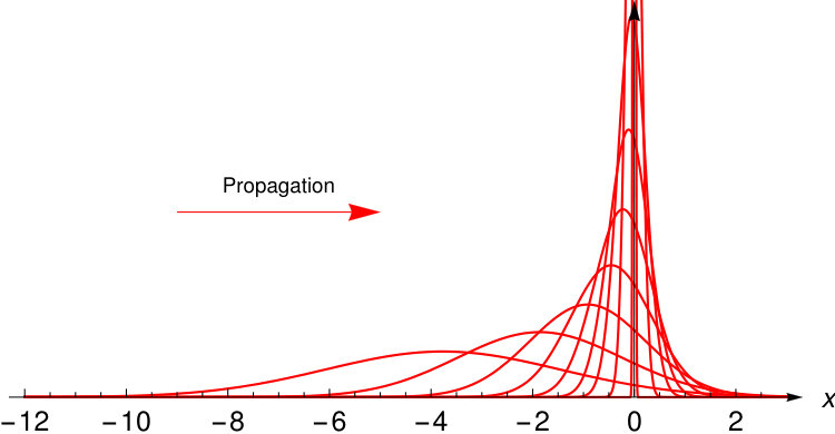 Figure 1
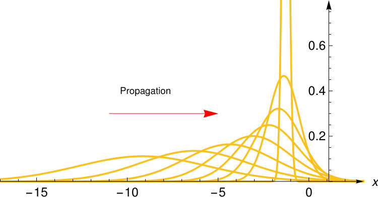 Figure 2
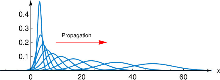 Figure 3
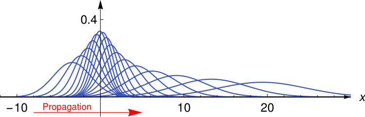 Figure 4
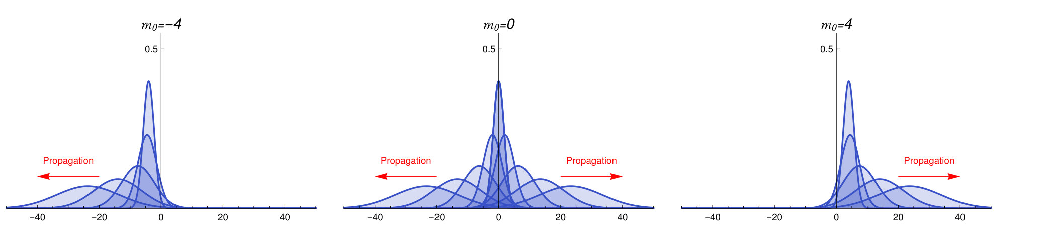 Figure 5
 Figure 6
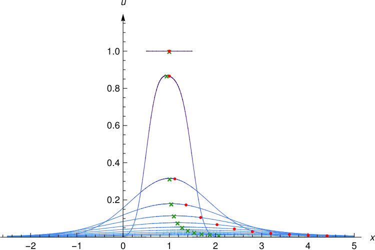 Figure 7
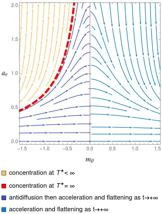 Figure 8
Peer Reviews
No public reviews on file for this paper yet. If you reviewed it on a platform where reviews are public (OpenReview, ICLR, NeurIPS, ICML), you can paste yours below so the community can read it here.
Videos
No videos yet. Explain this paper in a talk, walkthrough, or lecture? Add one.
Density dependent replicator-mutator models in directed evolution
Matthieu Alfaro and Mario Veruete
imag, Université de Montpellier, cnrs, Montpellier, France.
Abstract.
We analyze a replicator-mutator model arising in the context of directed evolution [23], where the selection term is modulated over time by the mean-fitness. We combine a Cumulant Generating Function approach [13] and a spatio-temporal rescaling related to the Avron-Herbst formula [1] to give of a complete picture of the Cauchy problem. Besides its well-posedness, we provide an implicit/explicit expression of the solution, and analyze its large time behaviour. As a by product, we also solve a replicator-mutator model where the mutation coefficient is socially determined, in the sense that it is modulated by the mean-fitness. The latter model reveals concentration or anti diffusion/diffusion phenomena.
Contents
1. Introduction
In this paper, we analyze a mathematical model of a directed evolution process which is density-dependent. The model in consideration is derived in [23] (see below for details) and is given by the following nonlocal equation
[TABLE]
where the nonlocal term is given by
[TABLE]
and will also be denoted , to remind its dependence on the solution itself. We will prove the well-posedness of the Cauchy problem associated with (1.1), obtain the solution through an implicit/explicit expression, and analyze its long time behaviour.
As a by product of our analysis of (1.1), we will collect results on the well-posedness and the long time behaviour of the solution to the Cauchy problem associated with equation
[TABLE]
where will also be denoted .
Throughout this work, we assume that the initial data and , are non-negative and have unitary mass
[TABLE]
so that, formally, for later times. Indeed, if we formally integrate (1.1) over , we see that the total mass solves the Cauchy problem
[TABLE]
so that, by the Cauchy-Lipschitz theorem, for all . Hence, is a probability density on and is its mean. As far as (1.3) is concerned, we reach
[TABLE]
so that, by Gronwall’s lemma, as long as “ is meaningful ”. We refer to [1] for situations where, in some sense, blows up in finite time, thus leading to extinction of the solution, which contradicts the formal conservation of the mass.
Let us now comment on the emergence of equations (1.1) and (1.3), termed as replicator-mutator models, in evolutionary biology and their relevance in biotechnology.
Replicator-mutator models aim at describing Darwinian evolutionary processes, whose fundamental elements are mutations and selection. Originally introduced by Taylor and Jonker [22], the replicator dynamics was developed for symmetric games in order to describe the evolution (determined by the payoff matrix) of the frequencies of strategies in a population, see [16] for a complete derivation. Nevertheless, such an approach neglects the effect of mutations. As an attempt to fill this gap, replicator-mutator models have been developed, starting with the work of Kimura [17] and followed by models considering different types of mutations, both in the local [6], [1, 2], [4] and nonlocal [17], [12], [8, 9, 10], [13, 14] cases.
It is important to mention the diversity of research areas where this type of model is applied: population genetics [15], game theory [7], auto-catalytic reaction networks [21] and language evolution [18]. As pointed out by Schuster and Sigmund [20], in the ordinary differential equation case, several evolutionary models in different biological fields lead independently to the same class of replicator dynamics, showing some sort of universal structure; this idea is also developed in [19], where authors show how apparently very different formulations of evolutionary dynamics are part of a single unified framework given by the replicator-mutator equation.
When mutations are modeled by the local diffusion operator, and under the constrain of mass, the replicator-mutator equation typically takes the form
[TABLE]
In the context of evolutionary biology, represents the density of population, at time , per unit of phenotypic trait on a one-dimensional phenotypic trait space. The function stands for the fitness of the phenotype and models the individual reproductive success. Hence the nonlocal term is the mean fitness at time , and can be seen as a Lagrange multiplier for the mass to be conserved, thus yielding an equation on the frequencies.
Due to their nonlocal structure, the analysis of replicator-mutator equations often requires new approaches compared with local-pde (e.g. comparison principle does not hold), both from the analytic and numerical viewpoint. In the framework of (1.7), we mention the works [2], [4] for the cases of quadratic or confining fitness functions, but now stick to the case where the fitness linearly depends on the phenotypic trait, say .
In this setting, the authors of [1] proved that the solution of the replicator mutator Cauchy problem (1.7) with linear fitness can be written explicitly in terms of the solution of the Heat equation. On the other hand, when a probability density (or kernel) models mutations, the equation is recast
[TABLE]
for which a Cumulant Generating Functions (CGF) approach has been developed in [13]: it turns out that the CGF satisfies a first order non-local partial differential equation that can be explicitly solved, thus giving access to many information such as mean fitness (or mean trait since ), variance, position of the leading edge. In the present paper, we shall combine these two techniques to first reach an implicit expression of the mean fitness of the solution to (1.1), and then to obtain a so called implicit/explicit expression of the solution itself. Additionally, this procedure allow us to develop a simple numerical strategy for solving the Cauchy problem associated to (1.1).
In this work, and in contrast with (1.7), we consider the case when the fitness function is modulated by , the mean-fitness at time , as can be seen in (1.1). Let us now make a short description of the emergence of model (1.1) in [23] to which we refer for further details.
The original mutator model, yielding the aforementioned replicator-mutator model (1.7), is the continuous time model
[TABLE]
and considers the so-called Malthusian fitness, that is the rate of growth of a particular genotype.
On the other hand, in the case of non-overlapping generations, one may start from the discrete time model
[TABLE]
for the change in the so-called Darwinian fitness (success in propagating genes to the next generation) distribution. The Darwinian fitness being nonnegative, equation (1.9) is supplemented with supported in . Model (1.9) is immediately recast
[TABLE]
Formally, at least for small times and narrow distributions, the above is approached by the continuous in time selection model
[TABLE]
which becomes (1.1) after inserting the effect of mutations through a diffusion term. Notice however that, in this derivation of (1.1), the fitness of an individual with trait depends only on and thus selection is not density dependent.
In [23], the authors consider directed evolution, that is a laboratory technique that mimics natural evolution and can be used for example to acquire proteins with new or improved properties. More precisely, they consider a high-throughput compartmentalized directed evolution process. Genotypes inside the compartments have different phenotypes. They not only pool their activity but also share the total number of produced copies, which makes the selection density dependent. In this process, the analogous of (1.9) is given by
[TABLE]
where the constant depends on , a Poisson parameter measuring the occupancy of compartments. The analogous of (1.10) is then
[TABLE]
Compared to (1.10), the presence of the coefficient in (1.13) is the revelator of the density dependent selection. Now, if is small (meaning large), the process is slowed down and the validity of (1.11) as a continuous in time approximation should hold in much more cases than previously, meaning for larger time periods but also for more various shapes of distribution.
Hence, the compartmentalization that takes place in directed evolution (but also in natural systems like viruses with multiple infections) and the associated frequency dependence are the key tools to reach the continuous time model (1.1), starting from a discrete time model written in terms of the Darwinian fitness, see [23].
Last, our second main focus, namely equation (1.3), corresponds to the replicator-mutator model (1.7), but with the additional effect that the mutations are frequency-dependent: the diffusion coefficient is modulated by the mean trait and is thus “socially determined”.
2. Main results
We here state our main results on (1.1), those on (1.3) will be gathered in the final section, where we transfer our developments on the solution of (1.1) to the solution of (1.3).
We first need to define an admissible set where to look after solutions. We denote by , the set of non-negative functions such that
[TABLE]
which decrease faster than any exponential function, that is
[TABLE]
and, last, such that
[TABLE]
Remark* 2.1**.*
Notice that the case follows by symmetry from the case , whereas the case is singular, as clear from the equation and the Gaussian case studied in subsection 3.2. Notice also that assumption (2.1) could be relaxed by only assuming limit when (or when ), the relevant tail being the right one as already observed in related situations by [1] or [13]. This would require to adapt in the below definition by adding some integrability properties as . For simplicity, in this work, we stick to (2.1).
Definition 2.2** (Notion of solution).**
Let be given. We say that is a global solution of (1.1) starting from if
, 2.
for all , , 3.
for all , , and decrease faster than any exponential function, in the sense of (2.1), 4.
* solves (1.1) in the classical sense,* 5.
* in , as .*
Our main result consists in the well-posedness of the Cauchy problem (1.1) with, moreover, an implicit/explicit expression of the solution.
Theorem 2.3** (The solution of the Cauchy problem).**
Let be given. Then there is a unique global solution of (1.1) starting from (in the sense of Definition 2.2). Moreover, its mean is implicitly (and uniquely) determined by
[TABLE]
where and , , is the cumulant generating function (cgf) of . Last, is given by
[TABLE]
where is the solution of the Heat equation starting from .
The proof is based in a combination of the approaches of [13] and [1]. In the course of the proof, we collect the expressions and some estimates on the mean and the variance
[TABLE]
of the solution at time .
Corollary 2.4** (Long time behaviour).**
Let be given. Then the mean of the global solution given by Theorem 2.3 satisfies
[TABLE]
and, in any case,
[TABLE]
The variance of the global solution satisfies
[TABLE]
where denotes the support of .
The above shows that, as , the solution moves to the right since , and is flattening since . In particular, for one side compactly supported initial data, the propagation (asymptotically) occurs at constant speed , which is in contrast with the acceleration phenomenon proved in [1]. This is also true for Gaussian data as will be noticed in subsection 3.2. The role of (2.2) is to provide “a kind of upper bound” on when, for example, the initial tails are still lighter than any exponential but heavier than Gaussian, e.g. of the magnitude () or even as .
The paper is organized as follows. In Section 3, we investigate special solutions, in particular Gaussian ones which provide a preliminary understanding of equation (1.1). In Section 4, we begin the proof of our main result, Theorem 2.3, by using the cgf approach introduced in [13]. The proof of Theorem 2.3 and its corollary are completed in Section 5 thanks to the methodology of [1]. As a by product of our analysis, we collect a numerical strategy for solving the Cauchy problem. Last, Section 6 is devoted to obtain the companion results on (1.3) by expressing in terms of .
3. Special solutions
In this section, we investigate special solutions to (1.1), in particular non-negative, integrable steady states and Gaussian solutions. In the first case we prove the non existence of such steady states. This is due to the particular form of the fitness function and is an analogous result to that one obtained by Alfaro an Carles in [1]. The situation is different in the case of a confining fitness function [4, 2] where the existence and uniqueness of a non-negative stationary solution is ensured and corresponds to the ground-state of the Schrödinger Hamiltonian where the potential is the opposite of fitness function. In the second case, Gaussian solutions are computed explicitly by solving the differential equations describing the evolution of the mean and the inverse of the variance.
3.1. Steady states
Proposition 3.1** (Steady state).**
There is no nontrivial non-negative steady state solving (1.1) and satisfying .
Proof.
A steady state with must solve for all . Letting , this is recast
[TABLE]
Hence is a linear combination of the Airy functions and . From , we deduce that is a multiple of . Hence either it is trivial, or it changes sign. ∎
3.2. Gaussian solutions
We investigate the propagation of a Gaussian initial data, which is relevant for biological applications. In the context of evolutionary genetics, families of Gaussian solutions for nonlinear and nonlocal equations can be found in [6], [1, 2]. In a different context involving logarithmic non-linearities, we also refer to [5], [11] for the Schrödinger equation and to [3] for the Heat equation.
Proposition 3.2** (Propagation of Gaussian initial data).**
For and , let us define
[TABLE]
Then
[TABLE]
solves (1.1) in and starts from u_{0}(x)=\mathchoice{{\hbox{\displaystyle\sqrt{\frac{a_{0}}{2\pi},}}\lower 0.4pt\hbox{\vrule height=9.3322pt,depth=-7.46579pt}}}{{\hbox{\textstyle\sqrt{\frac{a_{0}}{2\pi},}}\lower 0.4pt\hbox{\vrule height=6.55832pt,depth=-5.24669pt}}}{{\hbox{\scriptstyle\sqrt{\frac{a_{0}}{2\pi},}}\lower 0.4pt\hbox{\vrule height=5.05275pt,depth=-4.04222pt}}}{{\hbox{\scriptscriptstyle\sqrt{\frac{a_{0}}{2\pi},}}\lower 0.4pt\hbox{\vrule height=5.05275pt,depth=-4.04222pt}}}e^{-a_{0}\frac{(x-m_{0})^{2}}{2}}.
Proof.
From the ansatz (3.2), we compute
[TABLE]
We plug the above into equation (1.1), and identify the , the and the coefficients to obtain three differential equations. The first one is
[TABLE]
whose solution, starting from , is given by the first part in (3.1). Using (3.3), we see that the two other equations reduce to , which is solved as
[TABLE]
and thus the second part in (3.1). ∎
Notice that functions and are respectively the mean and the variance of the density . Hence Proposition 3.2 shows that, starting from a Gaussian profile, the solution remains a Gaussian function, is asymptotically propagating at constant speed and flattening since m(t)\sim\pm\mathchoice{{\hbox{\displaystyle\sqrt{2\sigma^{2},}}\lower 0.4pt\hbox{\vrule height=6.44444pt,depth=-5.15558pt}}}{{\hbox{\textstyle\sqrt{2\sigma^{2},}}\lower 0.4pt\hbox{\vrule height=6.44444pt,depth=-5.15558pt}}}{{\hbox{\scriptstyle\sqrt{2\sigma^{2},}}\lower 0.4pt\hbox{\vrule height=4.51111pt,depth=-3.6089pt}}}{{\hbox{\scriptscriptstyle\sqrt{2\sigma^{2},}}\lower 0.4pt\hbox{\vrule height=3.44165pt,depth=-2.75334pt}}}\,t, , as , see Figure 1. Notice that the direction of propagation is determined by the initial value : towards the right when , the left when . The case is singular because of the multiplicity of solutions to (3.1), two Gaussian solutions emerge, propagating to the left and to the right, see Figure 1.
4. The CGF approach
In this section, we assume that we are equipped with a solution of (1.1) starting from . We define the Cumulative Generating Function (cgf)
[TABLE]
of such a solution, in the spirit of [13]. From Definition 2.2, is well defined and smooth on . We shall derive an implicit expression for , and then for the value of the mean. This crucial step will enable us to complete the analysis in the next section, which is much in the spirit of [1].
The following computations are validated by the notion of solution adopted in Definition 2.2 and, possibly, the dominated convergence theorem. Observe that
[TABLE]
and that
[TABLE]
Notice in particular that the mean is reached through
[TABLE]
whereas the variance is reached through
[TABLE]
Hence, multiplying equation (1.1) by , integrating over and finally dividing by , we obtain the following nonlocal first order pde
[TABLE]
where we have used integration by parts to get
[TABLE]
Furthermore, since , the condition must hold for any . As a result we are facing the problem
[TABLE]
where is the cgf of the initial data . Notice that, from a straightforward computation,
[TABLE]
Hence, from Cauchy Schwarz inequality, we see that for all , and even for all if . This convexity property of cumulant generating functions is well-known in probability, and will be used in the following.
Fix and . For such that and , set
[TABLE]
which we differentiate to get
[TABLE]
As a result,
[TABLE]
From (4.4), we deduce that
[TABLE]
by Fubini-Tonelli theorem. We thus conclude that
[TABLE]
This is an implicit expression for since it still involves . Differentiating with respect to and evaluating at , we reach another implicit formula for the mean value of the solution
[TABLE]
whereas differentiating twice with respect to and evaluating at , we reach the variance of the solution
[TABLE]
where the last estimate follows from [13, Lemma 4.5].
Next, differentiating (4.5) with respect to , we get
[TABLE]
so that and thus
[TABLE]
Also, integrating , we collect the very useful expression
[TABLE]
Remark* 4.1**.*
Notice that if u_{0}(x)=\mathchoice{{\hbox{\displaystyle\sqrt{\frac{a_{0}}{2\pi},}}\lower 0.4pt\hbox{\vrule height=9.3322pt,depth=-7.46579pt}}}{{\hbox{\textstyle\sqrt{\frac{a_{0}}{2\pi},}}\lower 0.4pt\hbox{\vrule height=6.55832pt,depth=-5.24669pt}}}{{\hbox{\scriptstyle\sqrt{\frac{a_{0}}{2\pi},}}\lower 0.4pt\hbox{\vrule height=5.05275pt,depth=-4.04222pt}}}{{\hbox{\scriptscriptstyle\sqrt{\frac{a_{0}}{2\pi},}}\lower 0.4pt\hbox{\vrule height=5.05275pt,depth=-4.04222pt}}}e^{-a_{0}\frac{(x-m_{0})^{2}}{2}} is a Gaussian initial data as in subsection 3.2, we know that its cgf is
[TABLE]
Hence \overline{u}(t)=\mathchoice{{\hbox{\displaystyle\sqrt{m_{0}^{2}+2\sigma^{2}t^{2}+\frac{2}{a_{0}}t,}}\lower 0.4pt\hbox{\vrule height=9.49944pt,depth=-7.59958pt}}}{{\hbox{\textstyle\sqrt{m_{0}^{2}+2\sigma^{2}t^{2}+\frac{2}{a_{0}}t,}}\lower 0.4pt\hbox{\vrule height=7.95523pt,depth=-6.36421pt}}}{{\hbox{\scriptstyle\sqrt{m_{0}^{2}+2\sigma^{2}t^{2}+\frac{2}{a_{0}}t,}}\lower 0.4pt\hbox{\vrule height=5.59444pt,depth=-4.47557pt}}}{{\hbox{\scriptscriptstyle\sqrt{m_{0}^{2}+2\sigma^{2}t^{2}+\frac{2}{a_{0}}t,}}\lower 0.4pt\hbox{\vrule height=4.94304pt,depth=-3.95445pt}}} and , which agrees with the values of and in Proposition 3.2.
5. The solution implicitly/explicitly
In this section, we mainly complete the proof of Theorem 2.3 and of Corollary 2.4. As a by product, we present some numerical strategies for solving (1.1).
First, assume that we are equipped with a solution of (1.1) starting from . In particular we know from Section 4 that is given by (4.8). Following [1], we write
[TABLE]
This clearly defines a unique , , , which has to satisfy
[TABLE]
We refer to [1] for more details on such a change of unknown function, which enables to reduce some replicator-mutator equations to the Heat equation.
Now, our main task is to show that the problem (4.8), is globally well-posed.
Lemma 5.1**.**
For any given , there is a unique solution to
[TABLE]
Proof.
Recall that . We define the following subspace of , equipped with the norm,
[TABLE]
which is a Banach space. Now, we define the operator , and is given by
[TABLE]
The proof consists in mimicking that of the Banach fixed point theorem. In order to prove existence, we introduce the sequence defined inductively by
[TABLE]
We have
[TABLE]
where . Then we straightforwardly prove by induction that, for any , any ,
[TABLE]
In particular, the series converges and therefore converges uniformly in to some which is a fixed point of .
As far as uniqueness is concerned, if and are two fixed points of then the argument to reach (5.5) also yields . Letting enforces . ∎
Completion of the proof of Theorem 2.3 and Corollary 2.4.
Hence, any solution in the sense of Definition 2.2 has to be given by (5.1), where is given by Lemma 5.1. Notice that, from (5.3), has to be smooth.
Conversely, it is now a matter of straightforward computations — based on (5.1),(5.2) and (5.3)— to check that this does provide the solution. Notice that, in particular, the initial data is understood in the sense of Definition 2.2 since, in the Cauchy problem for the heat equation (5.2), the initial data is understood in the sense in as . This proves Theorem 2.3.
Last, the conclusions of Corollary 2.4 have been collected in the course of Section 4, except estimate (2.2) which will be obtained in the proof of Lemma 6.3, where its relevance will become much clearer. ∎
Numerical implications. Three major difficulties are encountered when setting up a numerical strategy for problem (1.1). The first one is the nonlocal nature of the equation. At this stage, two natural approaches can be considered: use finite differences and approximate the nonlocal term by a Riemann sum; apply a splitting method, computing alternatively the solution of the non-local term and the resulting local reaction-diffusion equation.
The second difficulty is the unboundedness of the domain. To manage it, one usually imposes artificial boundary conditions and solves numerically the equation on a sufficiently large domain, approximating the true solution by the latter.
The third complexity comes from the propagation of the solution, at least linear in view of (4.7), making it difficult to track it over time.
Previously, we gave an implicit/explicit construction of the solution of the Cauchy problem associated with equation (1.1), which actually provides a strategy for solving numerically the problem.
The idea is to initially find an approximation of the nonlocal term on a time interval . This step is performed using the fixed-point iteration sequence (5.4), for which the estimate (5.5) provides a convergence rate. This requires in particular to compute (analytically or numerically) the cumulant generating function of the initial datum .
The next step consists in calculating the solution of the heat equation with initial datum and evaluating it in the values indicated by formula (5.1). Obviously, in the case where an explicit solution of the heat equation can be found, artificial boundary conditions for solving the heat equation are not needed, leading to a better numerical solution. On the other hand, in the case where no closed form for is available, it is important to previously solve numerically the heat equation in a sufficiently large spatial domain. For instance, if we want to solve numerically (1.1) in , assuming (the case following by symmetry), then it is clear from (5.1) that the function needs to be evaluated in space up to and since , then we should solve the heat equation at most in .
In figure 2(b), we have represented the numerical solution obtained by this method for the initial condition , so that and , and ; in this case, is known to be given by
[TABLE]
6. When the mutation coefficient is socially determined
This section is devoted to the analysis of equation (1.3) supplemented with a non-negative initial data satisfying , and decreasing faster than any exponential data in the sense of (2.1). We denote . Interestingly, one can avoid the assumption in subsection 6.1 and obtain anti-diffusing/diffusing solutions that are mathematically interesting.
6.1. Gaussian solutions: concentration vs. extinction
Proposition 6.1** (Propagation of Gaussian initial data).**
For and . Then there is a unique Gaussian
[TABLE]
which solves, at least locally in time, (1.3) and starts from u_{0}(x)=\mathchoice{{\hbox{\displaystyle\sqrt{\frac{a_{0}}{2\pi},}}\lower 0.4pt\hbox{\vrule height=9.3322pt,depth=-7.46579pt}}}{{\hbox{\textstyle\sqrt{\frac{a_{0}}{2\pi},}}\lower 0.4pt\hbox{\vrule height=6.55832pt,depth=-5.24669pt}}}{{\hbox{\scriptstyle\sqrt{\frac{a_{0}}{2\pi},}}\lower 0.4pt\hbox{\vrule height=5.05275pt,depth=-4.04222pt}}}{{\hbox{\scriptscriptstyle\sqrt{\frac{a_{0}}{2\pi},}}\lower 0.4pt\hbox{\vrule height=5.05275pt,depth=-4.04222pt}}}e^{-a_{0}\frac{(x-m_{0})^{2}}{2}}. Its behaviour depends strongly on the parameters , and .
Assume m_{0}<-\frac{1}{a_{0}\mathchoice{{\hbox{\displaystyle\sqrt{2\sigma^{2},}}\lower 0.4pt\hbox{\vrule height=4.51111pt,depth=-3.6089pt}}}{{\hbox{\textstyle\sqrt{2\sigma^{2},}}\lower 0.4pt\hbox{\vrule height=4.51111pt,depth=-3.6089pt}}}{{\hbox{\scriptstyle\sqrt{2\sigma^{2},}}\lower 0.4pt\hbox{\vrule height=3.15778pt,depth=-2.52625pt}}}{{\hbox{\scriptscriptstyle\sqrt{2\sigma^{2},}}\lower 0.4pt\hbox{\vrule height=2.40916pt,depth=-1.92735pt}}}}. Then blows up in finite time: there is such that
[TABLE] 2.
Assume m_{0}=-\frac{1}{a_{0}\mathchoice{{\hbox{\displaystyle\sqrt{2\sigma^{2},}}\lower 0.4pt\hbox{\vrule height=4.51111pt,depth=-3.6089pt}}}{{\hbox{\textstyle\sqrt{2\sigma^{2},}}\lower 0.4pt\hbox{\vrule height=4.51111pt,depth=-3.6089pt}}}{{\hbox{\scriptstyle\sqrt{2\sigma^{2},}}\lower 0.4pt\hbox{\vrule height=3.15778pt,depth=-2.52625pt}}}{{\hbox{\scriptscriptstyle\sqrt{2\sigma^{2},}}\lower 0.4pt\hbox{\vrule height=2.40916pt,depth=-1.92735pt}}}}. Then and are global and
[TABLE] 3.
Assume m_{0}>-\frac{1}{a_{0}\mathchoice{{\hbox{\displaystyle\sqrt{2\sigma^{2},}}\lower 0.4pt\hbox{\vrule height=4.51111pt,depth=-3.6089pt}}}{{\hbox{\textstyle\sqrt{2\sigma^{2},}}\lower 0.4pt\hbox{\vrule height=4.51111pt,depth=-3.6089pt}}}{{\hbox{\scriptstyle\sqrt{2\sigma^{2},}}\lower 0.4pt\hbox{\vrule height=3.15778pt,depth=-2.52625pt}}}{{\hbox{\scriptscriptstyle\sqrt{2\sigma^{2},}}\lower 0.4pt\hbox{\vrule height=2.40916pt,depth=-1.92735pt}}}}. Then and are global and
[TABLE]
where C_{m}:=\frac{2a_{0}m_{0}\mathchoice{{\hbox{\displaystyle\sqrt{\sigma^{2},}}\lower 0.4pt\hbox{\vrule height=4.277pt,depth=-3.42162pt}}}{{\hbox{\textstyle\sqrt{\sigma^{2},}}\lower 0.4pt\hbox{\vrule height=4.277pt,depth=-3.42162pt}}}{{\hbox{\scriptstyle\sqrt{\sigma^{2},}}\lower 0.4pt\hbox{\vrule height=3.01193pt,depth=-2.40956pt}}}{{\hbox{\scriptscriptstyle\sqrt{\sigma^{2},}}\lower 0.4pt\hbox{\vrule height=2.40916pt,depth=-1.92735pt}}}+\mathchoice{{\hbox{\displaystyle\sqrt{2,}}\lower 0.4pt\hbox{\vrule height=4.51111pt,depth=-3.6089pt}}}{{\hbox{\textstyle\sqrt{2,}}\lower 0.4pt\hbox{\vrule height=4.51111pt,depth=-3.6089pt}}}{{\hbox{\scriptstyle\sqrt{2,}}\lower 0.4pt\hbox{\vrule height=3.15778pt,depth=-2.52625pt}}}{{\hbox{\scriptscriptstyle\sqrt{2,}}\lower 0.4pt\hbox{\vrule height=2.25555pt,depth=-1.80446pt}}}}{4a_{0}\mathchoice{{\hbox{\displaystyle\sqrt{\sigma^{2},}}\lower 0.4pt\hbox{\vrule height=4.277pt,depth=-3.42162pt}}}{{\hbox{\textstyle\sqrt{\sigma^{2},}}\lower 0.4pt\hbox{\vrule height=4.277pt,depth=-3.42162pt}}}{{\hbox{\scriptstyle\sqrt{\sigma^{2},}}\lower 0.4pt\hbox{\vrule height=3.01193pt,depth=-2.40956pt}}}{{\hbox{\scriptscriptstyle\sqrt{\sigma^{2},}}\lower 0.4pt\hbox{\vrule height=2.40916pt,depth=-1.92735pt}}}}>0 and C_{V}:=\frac{2a_{0}m_{0}\mathchoice{{\hbox{\displaystyle\sqrt{\sigma^{2},}}\lower 0.4pt\hbox{\vrule height=4.277pt,depth=-3.42162pt}}}{{\hbox{\textstyle\sqrt{\sigma^{2},}}\lower 0.4pt\hbox{\vrule height=4.277pt,depth=-3.42162pt}}}{{\hbox{\scriptstyle\sqrt{\sigma^{2},}}\lower 0.4pt\hbox{\vrule height=3.01193pt,depth=-2.40956pt}}}{{\hbox{\scriptscriptstyle\sqrt{\sigma^{2},}}\lower 0.4pt\hbox{\vrule height=2.40916pt,depth=-1.92735pt}}}+\mathchoice{{\hbox{\displaystyle\sqrt{2,}}\lower 0.4pt\hbox{\vrule height=4.51111pt,depth=-3.6089pt}}}{{\hbox{\textstyle\sqrt{2,}}\lower 0.4pt\hbox{\vrule height=4.51111pt,depth=-3.6089pt}}}{{\hbox{\scriptstyle\sqrt{2,}}\lower 0.4pt\hbox{\vrule height=3.15778pt,depth=-2.52625pt}}}{{\hbox{\scriptscriptstyle\sqrt{2,}}\lower 0.4pt\hbox{\vrule height=2.25555pt,depth=-1.80446pt}}}}{2\mathchoice{{\hbox{\displaystyle\sqrt{2,}}\lower 0.4pt\hbox{\vrule height=4.51111pt,depth=-3.6089pt}}}{{\hbox{\textstyle\sqrt{2,}}\lower 0.4pt\hbox{\vrule height=4.51111pt,depth=-3.6089pt}}}{{\hbox{\scriptstyle\sqrt{2,}}\lower 0.4pt\hbox{\vrule height=3.15778pt,depth=-2.52625pt}}}{{\hbox{\scriptscriptstyle\sqrt{2,}}\lower 0.4pt\hbox{\vrule height=2.25555pt,depth=-1.80446pt}}}a_{0}}>0.
Remark* 6.2**.*
In Figure 3, we have subdivided the phase plane into regions corresponding to the cases and .
Case corresponds to a concentration phenomena in finite time: the Gaussian solution converges, in finite time, to a Dirac mass centered at . See Figure 4.
Case corresponds to a concentration phenomena in infinite time: the Gaussian solution converges, at large times, to a Dirac mass centered at . See Figure 5.
In case , if then, in contrast with cases and , the mean of the solution manages to “cross” the value zero. In case convergence to a accelerating (m(t)\sim C_{m}e^{\mathchoice{{\hbox{\displaystyle\sqrt{2\sigma^{2},}}\lower 0.4pt\hbox{\vrule height=4.51111pt,depth=-3.6089pt}}}{{\hbox{\textstyle\sqrt{2\sigma^{2},}}\lower 0.4pt\hbox{\vrule height=4.51111pt,depth=-3.6089pt}}}{{\hbox{\scriptstyle\sqrt{2\sigma^{2},}}\lower 0.4pt\hbox{\vrule height=3.15778pt,depth=-2.52625pt}}}{{\hbox{\scriptscriptstyle\sqrt{2\sigma^{2},}}\lower 0.4pt\hbox{\vrule height=2.40916pt,depth=-1.92735pt}}}t}) and flattening (V(t)\sim C_{V}e^{\mathchoice{{\hbox{\displaystyle\sqrt{2\sigma^{2},}}\lower 0.4pt\hbox{\vrule height=4.51111pt,depth=-3.6089pt}}}{{\hbox{\textstyle\sqrt{2\sigma^{2},}}\lower 0.4pt\hbox{\vrule height=4.51111pt,depth=-3.6089pt}}}{{\hbox{\scriptstyle\sqrt{2\sigma^{2},}}\lower 0.4pt\hbox{\vrule height=3.15778pt,depth=-2.52625pt}}}{{\hbox{\scriptscriptstyle\sqrt{2\sigma^{2},}}\lower 0.4pt\hbox{\vrule height=2.40916pt,depth=-1.92735pt}}}t}) profile always occurs at large times. Moreover, the variance of the solution is decreasing before the mean reaches zero, and then starts to increase after the mean crosses zero, which reveals an anti-diffusion/diffusion phenomenon, see Figure 6. On the other hand, if , the solution does not anti-diffuse and only diffuses while the mean tends to infinity, see Figure 7.
Proof.
As in the proof of Proposition 3.2, we plug the ansatz (6.1) into (1.3) and arrive at
[TABLE]
so that , , which is globally solved as
[TABLE]
From the first equation in (6.2) we deduce
[TABLE]
as long as blow-up does not occur. We now easily see that in case blow up occurs at time
[TABLE]
In case blow up does not occur, m(t)=m_{0}e^{-\mathchoice{{\hbox{\displaystyle\sqrt{2\sigma^{2},}}\lower 0.4pt\hbox{\vrule height=4.51111pt,depth=-3.6089pt}}}{{\hbox{\textstyle\sqrt{2\sigma^{2},}}\lower 0.4pt\hbox{\vrule height=4.51111pt,depth=-3.6089pt}}}{{\hbox{\scriptstyle\sqrt{2\sigma^{2},}}\lower 0.4pt\hbox{\vrule height=3.15778pt,depth=-2.52625pt}}}{{\hbox{\scriptscriptstyle\sqrt{2\sigma^{2},}}\lower 0.4pt\hbox{\vrule height=2.40916pt,depth=-1.92735pt}}}t} and a(t)=a_{0}e^{\mathchoice{{\hbox{\displaystyle\sqrt{2\sigma^{2},}}\lower 0.4pt\hbox{\vrule height=4.51111pt,depth=-3.6089pt}}}{{\hbox{\textstyle\sqrt{2\sigma^{2},}}\lower 0.4pt\hbox{\vrule height=4.51111pt,depth=-3.6089pt}}}{{\hbox{\scriptstyle\sqrt{2\sigma^{2},}}\lower 0.4pt\hbox{\vrule height=3.15778pt,depth=-2.52625pt}}}{{\hbox{\scriptscriptstyle\sqrt{2\sigma^{2},}}\lower 0.4pt\hbox{\vrule height=2.40916pt,depth=-1.92735pt}}}t}. In case blow up does not occur and conclusion follows from (6.3) and (6.4). ∎
6.2. General solutions
Here we consider a non-negative initial data satisfying , (2.1) and , and investigate possible solutions of (1.3) starting from . From Theorem 2.3, we are equipped with the unique solution of equation (1.1) starting from . Roughly speaking, the understanding of (1.3) now reduces to that of the o.d.e. Cauchy problem
[TABLE]
Indeed, defining
[TABLE]
we have and one checks that, since solves (1.1) (and starts from ), solves (1.3) (and starts from ) as long as the solution of (6.5) exists.
Lemma 6.3**.**
The solution of the o.d.e. Cauchy problem (6.5) is global.
Proof.
If blows up in finite time, say at time , then we obtain from the o.d.e. that
[TABLE]
Hence we deduce from (4.5) that
[TABLE]
But, from (4.8), we know that \frac{y}{\overline{u}(y)}\leq\frac{1}{\mathchoice{{\hbox{\displaystyle\sqrt{2\sigma^{2},}}\lower 0.4pt\hbox{\vrule height=4.51111pt,depth=-3.6089pt}}}{{\hbox{\textstyle\sqrt{2\sigma^{2},}}\lower 0.4pt\hbox{\vrule height=4.51111pt,depth=-3.6089pt}}}{{\hbox{\scriptstyle\sqrt{2\sigma^{2},}}\lower 0.4pt\hbox{\vrule height=3.15778pt,depth=-2.52625pt}}}{{\hbox{\scriptscriptstyle\sqrt{2\sigma^{2},}}\lower 0.4pt\hbox{\vrule height=2.40916pt,depth=-1.92735pt}}}} and thus
[TABLE]
which contradicts . This concludes the proof of the lemma and, clearly, of estimate (2.2). ∎
Since is smooth, so is . Also, and, in particular, tends to as . Hence is a smooth diffeomorphism. In other words, (6.6) shows that there is a one-to-one correspondence between solutions to (1.3) and that of (1.1). We omit the full details but this clearly concludes the analysis of the Cauchy problem associated with (1.3), whose surprising qualitative behaviours have already been underlined in subsection 6.1.
Acknowledgements. The authors are very grateful to Anton Zadorin for sharing his expertise on the models appearing in [23], and for a precise relecture of the preprint, in particular the introduction. M. Alfaro is supported by the ANR i-site muse, project michel 170544IA (n*∘* ANR idex-0006). M. Veruete is supported by the National Council for Science and Technology of Mexico.
The reference list from the paper itself. Each links out to its DOI / PubMed record.
- 1[1] M. Alfaro and R. Carles , Explicit solutions for replicator-mutator equations: extinction versus acceleration , SIAM J. Appl. Math., 74 (2014), pp. 1919–1934.
- 2[2] M. Alfaro and R. Carles , Replicator-mutator equations with quadratic fitness , Proc. Amer. Math. Soc., 145 (2017), pp. 5315–5327.
- 3[3] M. Alfaro and R. Carles , Superexponential growth or decay in the heat equation with a logarithmic nonlinearity , Dyn. Partial Differ. Equ., 14 (2017), pp. 343–358.
- 4[4] M. Alfaro and M. Veruete , Evolutionary branching via replicator–mutator equations , J. Dynam. Differential Equations, (2018).
- 5[5] I. Białynicki-Birula and J. Mycielski , Nonlinear wave mechanics , Ann. Physics, 100 (1976), pp. 62–93.
- 6[6] V. N. Biktashev , A simple mathematical model of gradual darwinian evolution: emergence of a gaussian trait distribution in adaptation along a fitness gradient , J. Math. Biol., 68 (2014), pp. 1225–1248.
- 7[7] I. Bomze and R. Burger , Stability by mutation in evolutionary games , Games Econom. Behav., 11 (1995), pp. 146–172.
- 8[8] R. Bürger , On the maintenance of genetic variation: global analysis of Kimura’s continuum-of-alleles model , J. Math. Biol., 24 (1986), pp. 341–351.